Efficient, Lightweight Cyber Intrusion Detection System for IoT Ecosystems Using MI2G Algorithm

Abstract

The increase in internet connectivity has led to an increased usage of the Internet of Things (IoT) and devices on the internet. These IoT devices are becoming the backbone of Industry 4.0. The dependence on IoT devices has made them vulnerable to cyber-attacks. IoT devices are often deployed in harsh conditions, challenged with less computational costs, and starved with energy. All these limitations make it tough to deploy accurate intrusion detection systems (IDSs) in IoT devices and make the critical IoT ecosystem more susceptible to cyber-attacks. A new lightweight IDS and a novel feature selection algorithm are introduced in this paper to overcome the challenges of computational cost and accuracy. The proposed algorithm is based on the Information Theory models to select the feature with high statistical dependence and entropy reduction in the dataset. This feature selection algorithm also showed an increase in performance parameters and a reduction in training time of 27–63% with different classifiers. The proposed IDS with the algorithm showed accuracy, Precision, Recall, and F1-Score of more than 99% when tested with the CICIDS2018 dataset. The proposed IDS is competitive in accuracy, Precision, Recall, and training time compared to the latest published research. The proposed IDS showed consistent performance on the UNSWNB15 dataset.

1. Introduction

Usage of the Internet has influenced all levels of society and industry. Industries struggling through productivity losses find refuge in automatic interaction and controlling devices using a web of devices connected over a network called the Internet of Things, commonly known as IoT. The dependence on IoT has increased the usage of networks and the density of cyber-attacks disrupting the operations of Industry 4.0, and the intrusions or cyber-attacks are ever-increasing [1,2,3]. These cyber-attacks aim to steal data, as in the case of a cyber-attack on the professional networking site LinkedIn [4], or disrupt the primary functioning of an organisation, affecting revenue and the supply chain; for example, Saudi Aramco SCM was stopped by a cyber-attack [5]. Sometimes, cyber-attacks can be so severe that they can impact a nation or a part of a nation—a cyber-attack on Iranian telecommunications disrupted 25% of the country’s internet [6]. Recent studies have shown that IoT can be exploited for data stealing, espionage, and cyber warfare, making the IoT susceptible to cyber-attacks [7]. Cyber-attacks have been ranked as one of the top five risks to organisations [8]. The number of cyber-attacks increased by 600% in 2020 [9], and attacks on the IoT are supposed to double by 2025, costing USD 10.5 trillion annually [10]. These attacks result in productivity loss, legal liabilities, and reputation loss in addition to financial loss [3,11,12]. The intrusion detection system (IDS) has been introduced to prevent cyber-attacks and avert the loss of data, unauthorised access, and unexpected behaviour of the systems. IDSs can distinguish between benign and malicious vectors and stop the intrusion into the network.

IDSs can be signature-based, anomaly-based, network-based, or a hybrid of any approach. The industry commonly uses two types of IDS: host- and network-based. Host-based intrusion detection systems (HIDSs) monitor individual devices and collect audit logs. In contrast, network-based intrusion detection systems (NIDSs) are not limited to any device and operate on the complete network. Both NIDSs and HIDSs capture and collect the audit logs. NIDSs are considered better than HIDSs because NIDSs are not limited to a device and can monitor the whole network, considered “wiretapping”. NIDSs unify the software with hardware to weed out malicious activities quicker than HIDSs. We considered the NIDS in this study by looking at the advantages of NIDS over HIDS. The IDS can be reactive in analysing the audit trails and logs. The common approach to taking action after an attack results in a detection rate of around 0.05%, and it takes at least 14 days to identify a cyber-attack [2]. Low detection rates and massive delays in detection warrant preventive and real-time system monitoring with the help of security protocols to identify the attacks. Recent IDSs adopt machine learning (ML) to increase accuracy and reduce identification time.

ML-based IDSs primarily use the K-Nearest Neighbour (kNN), K-Means Clustering, Support Vector Machine (SVM), neural networks, and Bayesian Networks. A few IDSs have been built using the Hidden Markov Model [13] and Self-Organizing Maps [14]. Various researchers have proposed Gaussian Naïve Bayes (NB), Decision Tree (DT), Logistic Regression (LR), and Random Forest (RF). Nevertheless, these models are afflicted with low accuracy. To overcome the low accuracy, some researchers have proposed the usage of neural networks (NN) such as Long Short-Term Memory (LSTM), Convulsion Neural Network (CNN), Recurrent Neural Network (RNN), and Restricted Boltzmann Machine (RBM). Various researchers have pointed out that ML and NN models are required to process a suitable volume of data for training and storage [15], thus requiring considerable memory and computational power to build and train the model [16,17,18].

All these ML models are based on the pretext that each vector contains a feature or combination of features that can be used to create a model and train it to capture the intrusion attacks. This high number of features usually leads to a vector having many features that may contain irrelevant and unimportant information [19]. Various researchers have proposed dimension reduction techniques and feature selection techniques to select the features for training the model. The dimension reduction techniques project the features onto a plane where the unwarranted dimensions are removed from the data, and ML models are trained. On the other hand, feature selection techniques create subsets of features and calculate the model’s accuracy. Features that give the highest accuracy are considered and extracted, or a direct relation between the feature and the target variable is calculated [20]. The feature subset that has an impact on the target variable is considered. Hence, extracting features helps reduce the inherent problems of bias and error in model creation [13,21,22]. However, most IoT systems are deployed at inaccessible, harsh locations and starved of storage and computational power. This indicates the need for an IDS for IoT that can work with less computational power and storage to safeguard IoT systems from cyber intrusions [23,24]. There are two challenges for an IDS for IoT to work efficiently

Firstly, a feature selection technique quickly provides the relevant and essential features and requires less computational power to find these features. Secondly, the element selected through the feature selection technique and the classifier should yield higher accuracy in less training time. Hence, targeted research providing industry-ready and low computational cost feature selection is needed IDS for IoT systems.

This study introduces the new feature selection technique called MI2G, which is based on Mutual Information, and Information Gain based on the critical concepts of the information theory. The study also introduces the IDS system for IoT using a decision tree (DT) and feature selection algorithm called MI2G. The proposed feature selection algorithm selects the feature which shows the high Mutual Information with the target feature and provides complete information about the elements in the dataset. The proposed system using MI2G also provide good accuracy with various datasets.

Our Contribution

The major contribution of the study is as follows:

• A novel, unique hybrid feature selection algorithm MI2G (Mutual Information-Information Gain) by amalgamating the Mutual Information and Information Gain techniques for feature selection.
• Novel lightweight, and less computation cost-intensive IDS system showing good accuracy on CICIDS2018 in reduced training time
• Present detailed experimental findings to understand the suggested strategy as a valuable, universal IoT ecosystem IDS solution technique.
• Verify proposed IDS with reduced dataset obtained by applying the new MI2G feature selection algorithm on CICIDS2018.
• Comparison of the Proposed IDS system with available recent studies with recent datasets CICIDS2018 dataset, and classical UNSWNB15 dataset. The proposed system showed comparable accuracy and other parameters in lesser time.

This research paper is organized as follows: after the introduction section, the rest of the article is divided into five sections. Section 2 describes the recent related work and introduces the background concepts on feature selection and classification techniques. Section 3 presents the MI2G algorithm, Section 4 defines the experimental setup, the dataset used in the study, and the steps involved in performing the analysis. The results are compared with the recently available studies in Section 5. Finally, the research paper concludes with future directions.

2. Related Work

This section discusses the few important recent research literature on IDS using various ML algorithms. The area discusses reduction techniques, autoencoders, deep learning techniques, filters, wrapper techniques, and information-theoretic-centric techniques in silos or hybrids for feature selection with various classification algorithms.

Zhang et al. [25] used the KDDCup99 dataset and NSL KDD data in the experiment, and three sets of experiments using GNB, PCA-GNB, and IPCA-GNB were carried out. With the help of PCA, the initial 41 features were reduced to 31. The authors also carried out the effect of the number of principal components 1–18 and found that accuracy decreases after six components. PCA GNB and IPCA-GNB reduced the time duration to 0.56 s and 0.5 s compared to 1.42 s of the NB model. Both models were able to reduce the time by 60% approximately to that of various SVM Models and increase accuracy to 86%.

Shen et al. [26] used the PCA and Linear Discriminant Analysis (LDA) to identify the features. They concluded that PCA is a linear dimensionality reduction tool and can be used for listing the most original features. At the same time, LDA is a nonlinear dimensionality reduction technique and provides the most discriminative feature from the list of features. They used the Gaussian Naïve Bayes classifier as the ML algorithm to classify the attack based on the PCA and LDA input. Their experiment was able to project an accuracy of 96% compared to SVM, kSVM of 82, and 90%, respectively. However, there is no mention of the time.

Abdulhamed et al. [27] have proposed a hybrid approach using an Autoencoder and PCA to reduce the feature. Autoencoders identify the elements in a nonlinear dataset, and PCA performs best for the linear features in a dataset. The authors evaluated the performance of the component using an RF classifier. They compared the version with the other studies using the feature selection techniques such as fisher scoring, KNN, DDR Feature, and XGBOOST. The AE-PCA RF achieved an accuracy of 99.5%, while KNN and XGBOOST had an accuracy of 99.7% and 98.5%, respectively. Li et al. [28] used three layers of Autoencoders for feature selection and Random Forest as the classifier. They were able to achieve an accuracy of 99% on their dataset. Additionally, they tried making the whole system lightweight and achieved good accuracy in less time using the KNN algorithm.

Lu and Tian [29] used a slightly different approach, using autoencoder as the feature selection technique and Bi-Directional LSTM as the classifier. Their experiment achieved an accuracy of 99.41% and a Precision of 99.14 on the KDDCUP 99 dataset. In this paper, the authors have compared the classification performance with that of the latest proposed classifiers and have found that it is comparable to or better than others.

Mayurnathan et al. [30] achieved an accuracy of the 99.92% with a sensitivity of 99.8% using the Randomised Harmony Search as a feature selection technique and Restricted Boltzmann Machines (RBM) as the classifier on a KDD CUP99 dataset. The proposed structure was able to outperform all the existing ML algorithms. Whitmire et al. [31] proposed using correlation-based and wrapper-based techniques for feature selection. They used various prediction algorithms such as SVR, DT, and LR to predict the yield of Alfafa. They proposed that CFS, in conjunction with SVR, was able to show the lowest MAE and RMSE. They highly recommend that CFS with SVR be used for the prediction techniques.

Alqahtani and Mathkour [32] proposed a new genetic-based XGBOOST algorithm with features selected through the Fisher Score. The model achieved an accuracy of 99.1% compared to the accuracy achieved by all markers with just two segments and achieved 100% accuracy with 3, 4, and 5 features. Additionally, the authors compared the accuracy with the latest research Comparison of results with related works for Mirai, Bashlite, and benign classification tasks with other studies showing 86.63% using DNN, 98.51 using DT, and KNN 97.24%, and proposed as 99.96%.

Saleh [33] used Information Gain, Gain Ratio, and Covariance as the feature selection. The feature set with 41 features of KDDCUP99 was used, and essential features 20, 28, 22 using the IG, GR, and Covariance. The top 2 features from each method were used, and a feature set of 6 features was made and subjected to a classifier using KNN, NB, and MLP, which in turn showed an accuracy of 98.9, 93.3, and 96.5, respectively. KDDCup99.

Mafarja et al. [23] achieved the accuracy of 99.41% on the self-generated data set of IoT by selecting the critical feature through the metaheuristic algorithm—Whale Optimisation Algorithm and kNN as the classifier. The authors did not perform any comparison with other meta-heuristic algorithms, such as PSO comparison.

Soleymanzadeh et al. [34] tried the ensemble technique for IDS. They tied the classifiers on the NSLKDD dataset and UNSWNB15 dataset and reported an accuracy of 95%. However, all these ensemble classifiers had an around 9–12 min training time. On the other hand, Carrera et al. [35] used the SHAP values for selecting the critical features and the autoencoders as classifiers. They proposed an IDS system with the Memory-Augmented Deep Autoencoder with Extended Isolation Forest classifier. Proposed IDS showed an accuracy of 95.14% for KDDCU99 and an accuracy of 83.5% for CICIDS2017.

Cao et al. [36] used the CNN and GRU using the hybrid feature selection technique Adaptive Synthetic Sampling (ADASYN) and Repeated Edited Nearest Neighbors (RENN). Their experiment showed the accuracy of UNSW_NB15 and NSL-KDD datasets, and the experimental results show that the classification accuracy reaches 86.25%, and 99.69%.

Kareem et al. [37] proposed a new feature selection technique GTO-BSA, which was based on the Gorilla Troops Optimizer (GTO) based on the algorithm for bird swarms (BSA). They obtained an accuracy of 98.7% on the CICIDS2018 dataset.

Imrana et al. [38] propose a novel feature-driven intrusion detection system, χ²-BidLSTM, that integrates a χ² statistical model and bidirectional long short-term memory (BidLSTM). They used the NSL KDD dataset and obtained an accuracy of 95.62%.

Jeyaselvi et al. [39] used the Improved Pearson Correlation Coefficient (IPCC) to identify features requiring less computational power and time and providing higher accuracy. Further, Hussein et al. [40] used the double feature selection technique on IoTID20 and showed accuracy in the range of 78.1% to 92% for features in the field of 20 to 25.

Table 1. Comparison of the latest related work.

Reference	FS Tech	FS Tech Type	Classification	Dataset	Accuracy	Training Time & Cost
[25]	GNB and PCA	Filter	SVM	KDDCup99	86%	High
[26]	PCA-LDA	Dimension Reduction	NB	CICIDS2017	96%	High
[27]	AE and PCA	Neural network + Dimension Reduction	XGBOOST	Self-Made	99%	Medium
[30]	RH Search	Wrapper	RBM	KDDCup99	99%	High
[23]	WHO	Wrapper	KNN	Self-Made	99%	High
[22]	KNN	Wrapper	ELM	NSLKDD	84%	High
[28]	AE and RF	Neural network + Wrapper	KNN	CICIDS2017	99%	High
[29]	AE	Neural Network	BD LSTM	KDDCup99	99%	High
[41]	GWO	Wrapper	SVM	NSLKDD	96%	High
[11]	Correlation	Filter	ANN	UNSW-NB15	98%	High
[31]	Correlation	Filter	SVM	Self-Made	98%	High

compares the amount of research carried out based on the technique used in the feature selection. It can be easily concluded that less research has been carried out on Information-centric and Filter based methods. Additionally, researchers have shown an affinity toward a hybrid feature selection technique. Most of them have used neural networks or autoencoders with any feature reduction or selection technique to obtain the essential features. Careful observation of the recent literature in Table 1 shows that most researchers [27,29,41] have used the first few critical features.

Nevertheless, in actuality, there could be a few features that individuals cannot cause any impact on, but collectively, they can influence the decision. Additionally, there might be a few features marked as necessary that are correlated to each other and do not cause any impact on the final accuracy of the intrusion detection system. Very little literature was available on using information-centric theory and filter-based techniques individually or in a hybrid framework for feature selection techniques [33]. A thorough analysis of the literature suggests that higher accuracy for a classifier can be obtained using the feature selection technique based on hybridization. Additionally, the available literature indicates that the information features selection technique uses less memory and computational cost than other techniques. The study is unique because it proposes the feature selection technique, which consumes less computational cost and provides features that help the classifiers accurately classify the attacks. The study provides a comprehensive analysis of IDS using Information Theory and a simple ML classifier (DT) to organize the data in the CICIDS2018 dataset. The proposed IDS also classifies the attacks with high accuracy and Precision in the lowest possible time.

3. Background

3.1. Mutual Information and Information Gain

Mutual Information (MI) defines the amount of dependence or information a random variable contains for the other random variable [42]. It can be further defined as reducing the uncertainty of the value of one random variable provided the value of other random variables. Consider X and Y to be two random variables in the space. Each variable’s probability mass functions as p(x) and p(y). Hence, Kullback–Leibler distance between these two mass functions is given as

$$\mathrm{I}\left(\mathrm{X};\mathrm{Y}\right)={{\displaystyle \sum }}_{\mathrm{x}\in \mathrm{Xy}\in \mathrm{Y}}^{.}\left(\mathrm{p}\left(\mathrm{x}\right)\mathrm{p}\left(\mathrm{y}\right)\log \frac{\mathrm{p}\left(\mathrm{x}\right)\left(\mathrm{y}\right)}{\mathrm{p}\left(\mathrm{x}\right)\mathrm{p}\left(\mathrm{y}\right)}\right)$$

(1)

$$\mathrm{I}\left(\mathrm{X};\mathrm{Y}\right)={{\displaystyle \sum }}_{\mathrm{x},\mathrm{y}}^{.}\left(\mathrm{p}\left(\mathrm{x},\mathrm{y}\right)\log \frac{\mathrm{p}(\mathrm{x}|\mathrm{y})}{\mathrm{p}\left(\mathrm{x}\right)\mathrm{p}\left(\mathrm{y}\right)}\right)$$

(2)

$$\mathrm{I}\left(\mathrm{X};\mathrm{Y}\right)=-{{\displaystyle \sum }}_{\mathrm{x},\mathrm{y}}^{.}\left(\mathrm{p}\left(\mathrm{x},\mathrm{y}\right)\log \mathrm{p}\left(\mathrm{x}\right)\right)+{{\displaystyle \sum }}_{\mathrm{x},\mathrm{y}}^{.}\left(\mathrm{p}\left(\mathrm{x},\mathrm{y}\right)\log \mathrm{p}\left(\mathrm{x}|\mathrm{y}\right)\right)$$

(3)

$$\mathrm{I}\left(\mathrm{X};\mathrm{Y}\right)=-{{\displaystyle \sum }}_{\mathrm{x},\mathrm{y}}^{.}\left(\mathrm{p}\left(\mathrm{x},\mathrm{y}\right)\log \mathrm{p}\left(\mathrm{x}\right)\right)-(-{{\displaystyle \sum }}_{\mathrm{x},\mathrm{y}}^{.}\left(\mathrm{p}\left(\mathrm{x},\mathrm{y}\right)\log \mathrm{p}\left(\mathrm{x}|\mathrm{y}\right)\right))$$

(4)

I (X;Y) = H(X) − H(X|Y)

(5)

By symmetry, it can be written that

I (X;Y) = H(Y) − H(Y|X)

(6)

Since

H(X,Y) = H(X) = H(Y|X)
I(X;Y) = H(X) + H(Y) − H(X,Y)

(7)

The entropy of the variable X is given by H(X) and H(Y). The entropy of X with a known Y value is given as H(X|Y), and the entropy of Y for any given value of X is given as H(Y|X). H(X|Y) can be called the conditional entropy of X over Y and vice versa. The joint entropy of the X and Y is given as H(X, Y). This can be represented in Figure 1.

Information Gain (IG) of a feature X defines the reduction in the entropy of dataset D by splitting the values on feature x or it can be explained as the variance caused by feature X. It can be calculated as the difference between the prior entropy of dataset D, and the conditional entropy of the dataset for the feature [42]. Hence, for any dataset D such that (x,y) = {x1, x2,………xn}, the IG can be given as

IG (D,x) = H(D) − H(D|x)

(8)

3.2. Classification Algorithms

Various machine learning algorithms such as kNN, DT, RF, and SVM have been applied in the IDS systems. Considering the merits and demerits of each ML algorithm discussed in Section 2. following ML classifiers were chosen for the study—LR, LDA, NB, DT, RF, SVM, and GBM. This section discusses and explains these classifiers.

Logistic regression (LR)—This is one of the oldest classifiers and is used for classifying the data in binary buckets, i.e., [0, 1]. It uses the sigmoid function as the activation function. For the feature vector X = { X1, X2, …, Xn }, the conditional probability of any vector to be assigned to bucket Y = 1 is given as below, where θ is the regression coefficient [43].

$$\mathrm{P} (\mathrm{Y}=1|\mathrm{X}1, \mathrm{X}2, \cdots , \mathrm{Xn})= \frac{\exp \left( \mathsf{\theta }0+\mathsf{\theta }1 \mathrm{X}1+\cdots +\mathsf{\theta }\mathrm{n} \mathrm{Xn}\right)}{1+\exp \left( \mathsf{\theta }0+\mathsf{\theta }1 \mathrm{X}1+\dots +\mathsf{\theta }\mathrm{n} \mathrm{Xn}\right)}$$

(9)

Linear Discriminant Analysis (LDA)—LDA uses the projection vector to increase the distance between the sample leading to different classes and reduces the distance between samples leading to the same class [44]. The projection vector of the LDA is calculated as below

$$a=\mathrm{argmax}\frac{{\mathrm{a}}^{\mathrm{T}}{\mathrm{s}}_{\mathrm{b}}\mathrm{a}}{{\mathrm{a}}^{\mathrm{T}}{\mathrm{s}}_{\mathrm{w}}\mathrm{a}}$$

(10)

where distance between vector is given by Sb, Sa, and a $\in$ A: A = {a1,a2,…….,an} $\in$ Rm × k.

Gaussian Naïve Bayes (NB)—This classification algorithm is based on the old naïve Bayes theorem of probability. It tries to find the probability of a vector falling into a labeled class. It considers that all events are independent of each other, assuming that posterior probability is a function of the likelihood of a last event [45].

$$\mathrm{P}\left({\mathrm{B}}_{\mathrm{i}}|\mathrm{A}\right)=\frac{\mathrm{P}\left({\mathrm{B}}_{\mathrm{i}}\right)\mathrm{P}\left({\mathrm{A}|\mathrm{B}}_{\mathrm{i}}\right)}{{{\displaystyle \sum }}_{\mathrm{i}=1}^{\mathrm{n}}\mathrm{P}\left({\mathrm{B}}_{\mathrm{i}}\right)\mathrm{P}\left({\mathrm{A}|\mathrm{B}}_{\mathrm{i}}\right)}$$

(11)

Support Vector Machine Algorithm (SVM)—This classification algorithm tries to separate the classes by a hyperplane [43,46]. The equation gives the hyperplanes.

$$\mathrm{f}\left(\mathrm{x}\right)=\left({\mathsf{\beta }}_0+{\mathsf{\beta }}_{\mathrm{t}}\mathrm{x}\right)$$

(12)

Here, β₀ is the bias, and β_t is the weight.

Decision Tree (DT)—DT is a supervised machine learning algorithm primarily used in classification problems. DT uses the concept of entropy or randomness and finds the best parameters which cause the increase or decrease in randomness for splitting the data. The entropy of a given feature is calculated using the below equation, where E (S) represents the entropy of the feature S, and pi is the probability [47].

$$\mathrm{E}\left(\mathrm{S}\right)={{\displaystyle \sum }}_{\mathrm{i}=1}^{\mathrm{n}}-{\mathrm{p}}_{\mathrm{i}}{\mathrm{logp}}_{\mathrm{i}}$$

(13)

Gradient Boosting ML algorithm (GBM)—GBM is a greedy algorithm that works on the ensemble of week learners such as CART. Each tree tries to reduce the mean square error between the actual and predicted values. Hence, the number of iterations is more, and the results are accurate. GBM is seen to be outperforming the RF algorithm [48,49].

Random Forest (RF)—RF algorithm is the ensemble of decision tree-based models which iteratively build a set of trees and choose the right tree to reduce the error. Like other tree-based models, it is also a greedy algorithm that shows good accuracy without overfitting [50].

4. Proposed MI2G Feature Selection Algorithm

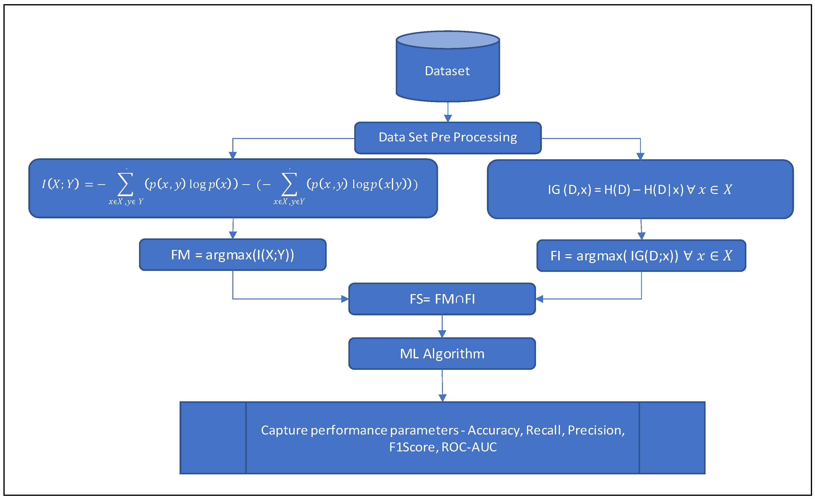
This section defines the feature selection algorithm MI2G algorithm, created by crossbreeding the two important information theory-centric models. The MI2G algorithm is applied to the feature vector F in the dataset such that F = {f₁, f₂, f₃,………., f_n} where F_k is an individual feature in the vector, and Y^T = {Y₁, Y₂….., Ym} represents the label of the attack such that Y_k $\in$ {0, 1}. MI2G finds out the best-selected feature set S such that S ⸦ F and maximises the accuracy of the classifier.

As the first step, each feature in F is normalised using MinMax scaling, which helps nullify the outliers. The entropy of each feature {f₁, f₂, f₃,………., f_n} with respect to label Y is calculated, which is further consumed to calculate the Kullback–Leibler distance or Mutual Information I (f_i, Y_i) (using Equation (7)) between each feature, and label Y. All the features which have argmax (I(f_i, Y_i)) are added to the list S1. The list S1 contains only a selected list of features that can relate to the outcome.

Similarly, each feature’s entropy and the complete dataset’s entropy are used to calculate the Information Gain IG (D|f_i) (using Equation (8)). Features providing the maximum information Gain is stored in the list S2. S1, and S2, both contain the name of the feature fi and the corresponding I (fi, Yi) value, and IG (D|f_i), respectively. The common feature from S1 and S2 are extracted and considered for the final selected feature set S.

The feature selection algorithm is computationally less expensive because it not only uses the simple calculations to find out the entropy of each feature, label, and complete dataset, but the entropies are also calculated once, which are used in calculating the I(fi, Yi), and IG (D|fi). Single-pass entropy calculations make the algorithm faster. The MI2G algorithm is further defined in Algorithm 1, and the schematic diagram of the algorithm is given in Figure 2 and Figure 3.

Algorithm 1: MI2G Algorithm

INPUT       F = {fi,f2,……. fn}       YT = {Y1,Y2…..,Ym} OUTPUT       S = {si,s2,……. sl} START {         //Initialize       S = Φ       S1 = Φ       S2 = Φ       //Normalise all the values in the dataset       FOR i in I where I ϵ {1,2,… n}       {          Normalize fi → fi = (fi − min (fi)/(max(fi)- min(fi))       }         // Find the MI and IG       FOR i ϵ { 1,2,3,… n}       {          I (fi,Y) = H (f1,Y) − H(f1|Y) − H(Y| f1)          IF argmaxfi (I(fi,Y)) where i = {1,2,…, n}             S1 = S1 U fi          END IF          IG (D|fi) = H (D) − H (D| fi)          IF argmaxfi (IG (D|fi)) where i = {1,2,…, n}             S2 = S1 U fi          END IF       }       //Find the commonly selected features       S ← S1 ∩ S2       RETURN S }

The proposed MI2G feature selection algorithm was tested with tuned classifiers LR, LDA, NB, SVM, DT, RF, and GBM as per the setup given in Section 5, and the results of each classifier with the initial dataset and selected feature are presented and discussed in Section 6.

5. Experimental Setup

This section introduces the experiments and steps taken to check the validity of the proposed MI2G algorithm for feature selection. It helps to identify the suitable classifier for the IDS system. In the current research, we applied the data preprocessing steps to remove the unidentified values and applied the transformation and normalization to ensure that good data leads to accurate results [34,35,36,37]. The dataset was split into a training set containing 80% and a validation set containing 20% of the complete dataset. The MI2G feature selection algorithm identified various machine learning algorithms’ relevant and essential features. Each machine learning algorithm was tuned using GridSearchCV to select the machine learning model with the best accuracy. The parameters for each model with the best accuracy are given in

Table 2. Hyperparameter and penalty for classifiers.

Classifier	Hyperparameters	Penalty
LR	C = 0.01, Solver = ‘liblinear’	L2
LDA	Solver = ‘lsqr’, Shrinkage = 0.81	L2
NB	var_smoothing = 0.05336699, alpha = 0.78	L2
DT	criterion = ‘entropy’, max_depth = 10, maxfeatures = log2	NA
RF	criterion = ‘entropy’, max_depth = 10, maxfeatures = log2, n_estimators = 1000	NA
SVM	C = 0.01, gamma = 0.023, kernel = ‘sigmoid’	L2
GBM	learning_rate = 0.001, max_depth = 11, max_features = log2, n_estimators = 1000	L2

. These models with the best parameters were applied to the validation set to verify the performance [38,39,40,51,52]. In order to avoid the overfitting of the model, models such as LR, LDA, SVM, GBM, and LDA were regularised using the L2 penalty. L2 penalty is susceptible to outliers, but it worked well in the current experiment because the dataset did not contain any outlier data [53,54,55,56]. The performance of ML algorithms was evaluated based on the criteria given in Table 3. On a high level, the complete experimental setup is depicted in Figure 2, and the schematic diagram of the proposed IDS system is given in Figure 3.

5.1. Data Set Cicids2018

The dataset CICIDS2018 was created by the Canadian Institute of Cybersecurity using the CICFlowmeter, V3Storm tool for creating the attack, and normal traffic vectors. The dataset contains the following attacks Brute-force, Heartbleed, Botnet, DoS, DDoS, Web attacks, and network infiltration from inside. These attacks were generated by attacking infrastructure with 50 machines and the victim organization with departments, including 420 machines and 30 servers. The dataset includes the captured network traffic and 80 features, including one label feature. The CICIDS2018 dataset is well accepted and has been used in various studies on IoT security.

The experiment used two instances of the CICIDS2018 dataset. The details of the instances are given as follows:

• Full Feature Dataset—This dataset has all 79 features and one label dataset of the CICIDS2018 dataset. This dataset is referred to as the entire dataset or initial dataset in this study, and this dataset is used for creating the initial performance baseline.
• Selected Important feature Dataset—This dataset contained 24 essential features from the CICIDS2018 dataset. The critical features were obtained using the MI2G algorithm and one label, and this dataset is referred to as the MI2G dataset in this study.

5.2. Pre-Processing

A sample dataset containing an equal number of ‘benign’ and ‘attack’ labels was deduced from the dataset to create a balanced dataset. The balanced dataset reduces the possibility for any model to overfit or underfit.

The features described in the last section were individually evaluated and verified that the feature value conforms to the definition. Most of the features with null and no defined values were filled with the most frequent values.

5.3. Data Normalization

Data normalization is a critical step in preparing data for any classification activity. The normalization remains an essential activity because it helps to reduce the range of data helping objective function, which usually does not work efficiently on a wide range of data. For this study, we followed the min–max normalization approach to ensure that data remains in the range of [0, 1], with 0 for the minimum and 1 for the maximum values

$$\mathrm{z}=\frac{\mathrm{x}-\mathrm{minimal}\left(\mathrm{x}\right)}{[\mathrm{maximal}\left(\mathrm{x}\right)-\mathrm{minimal}\left(\mathrm{x}\right)]}$$

(14)

The normalisation was applied to each feature of the dataset.

5.4. Performance Evaluation Criteria

For evaluating the proposed system’s performance and comparing it with existing published research, the following parameters were measured or calculated.

Accuracy can be defined as the ratio of correctly classified instances to total classified instances. It can be given as below

$$\mathrm{Accuracy}=\frac{\mathrm{TP} + \mathrm{TN}}{\mathrm{TP} + \mathrm{FP} + \mathrm{TN} + \mathrm{FN}}$$

(15)

Precision can be defined as the ratio of instances correctly classified as an attack to that of instances identified as attacks. It can be given as below

$$\mathrm{Precision}=\frac{\mathrm{TP}}{\mathrm{TP} + \mathrm{FP}}$$

(16)

Recall can be defined as the ratio of instances correctly classified as an attack to those that are attacked. It can be given as below

$$\mathrm{Recall}=\frac{\mathrm{TP}}{\mathrm{TP} + \mathrm{FN}}$$

(17)

F1-Score can be defined as the harmonic mean of Precision and Recall. It can be given as below

$$\mathrm{F}1-\mathrm{Score}=2\times \frac{\mathrm{Precision} \times \mathrm{Recall}}{\mathrm{Precision} + \mathrm{Recall}}$$

(18)

These parameters are measured for the proposed IDS and various ML algorithms and are discussed in the next section.

6. Results and Discussions

This section talks about the results obtained during the experiments. The experiments were carried out with the original data with full features and were processed using techniques such as filling the missing values, not identified values, and other processing techniques described earlier. The processed and normalized dataset was applied to a few essential classifiers in Section 2, and the parameters given in Section 5.4 were obtained. The results are given in Table 3, which suggests that the least training time was taken Gaussian Naïve Bayes classifier, and the Support Vector Machine took the highest time. While SVM took the highest time to train the classifier, DT and RF took just 0.67 s and 0.58 s, respectively. The decision tree and Random Forest showed excellent accuracy, approximately 96.5% and 96.8%, respectively. NB showed an accuracy of approximately 71.51%. The GBM classifier exhibited the second-best accuracy, with 94.78%. The LR, LDA, and SVM showed an accuracy of 89.32%, 84.36%, and 76.8%, respectively. Both DT and RF showed more accuracy than an F1-Score of 96.21% and 96.23%, respectively.

On the other hand, NB showed the most miniature Precision, the F1-Score value with values around 72%, and the lowest Recall with 71.51%. RF took slightly lesser training time than DT to show comparable accuracy, Precision, and Recall. Analyzing Table 3, it can be easily concluded that RF and DT are best suited for identifying an attack on any IoT system.

Table 3. Performance parameter for the full dataset—CICIDS2018.

Classifier Name	Train Time	Test Time	Accuracy	Precision	Recall	F1-Score
LR	5.02	0.03	89.32	89.21	89.29	89.25
LDA	0.58	0.018	84.36	84.32	84.56	84.44
NB	0.05	0.02	71.51	72.01	71.51	71.76
DT	0.67	0.013	96.49	96.19	96.23	96.21
RF	0.58	0.029	96.86	95.88	96.59	96.23
SVM	11.32	0.38	76.8	76.9	77.18	77.04
GBM	7.95	0.06	94.78	93.21	94.15	93.68

Table 3. Performance parameter for the full dataset—CICIDS2018.

Classifier Name	Train Time	Test Time	Accuracy	Precision	Recall	F1-Score
LR	5.02	0.03	89.32	89.21	89.29	89.25
LDA	0.58	0.018	84.36	84.32	84.56	84.44
NB	0.05	0.02	71.51	72.01	71.51	71.76
DT	0.67	0.013	96.49	96.19	96.23	96.21
RF	0.58	0.029	96.86	95.88	96.59	96.23
SVM	11.32	0.38	76.8	76.9	77.18	77.04
GBM	7.95	0.06	94.78	93.21	94.15	93.68

The MI2G feature selection algorithm was applied to the dataset, and essential features were selected, as shown in

Table 4. Features selected through the MI2G algorithm.

Feature selected by MI2G algorithm

Fwd_Packets_s, Flow_Packets_s, Flow_IAT_Mean, Destination_Port, Bwd_Packets_s, Flow_Bytes_s, Fwd_IAT_Mean, Flow_IAT_Max, Fwd_Packet_Length_Mean, Avg_Fwd_Segment_Size, Packet_Length_Std, Fwd_Header_Length, Packet_Length_Variance, Total_Length_of_Fwd_Packets, Subfow_Fwd_Bytes, Packet_Length_Mean, Fwd_Packet_Length_Max, Bwd_Packet_Length_Mean, Avg_Bwd_Segment_Size, Total_Length_of_Bwd_Packets, Fwd_IAT_Total, Bwd_IAT_Total, Bwd_IAT_Max, Fwd_IAT_Max

. A newly built dataset from the CICIDS2018 dataset for features selected through MI2G was created and applied to the classification algorithms. Performance parameters were obtained, as shown in

Table 5. Performance parameter for the feature selected through MI2G dataset extracted from CICIDS2018.

Classifier Name	Train Time	Test Time	Accuracy	Precision	Recall	F1-Score
LR	1.83	0.01	91.81	91.8	91.7	91.75
LDA	0.29	0.01	87.66	87.6	86.5	87.05
NB	0.02	0.011	75.19	79.9	75.22	77.49
DT	0.39	0.009	99.68	99.58	99.65	99.61
RF	0.41	0.021	99.37	99.13	99.51	99.32
SVM	8.41	0.31	80.74	80.46	80.36	80.41
GBM	5.49	0.05	98.89	98.81	98.81	98.81

. Figure 4 shows that the MI2G algorithm considerably reduced the training time and testing time of all the algorithms while increasing or retaining the accuracy, Precision, Recall, and F1-Score for all the classification algorithms. The proposed MI2G algorithm reduced the training time by approximately 25% to 63%, and a similar trend was seen in the case of testing time. LR showed a reduction of 63% in training time and 67% in testing time with the proposed MI2G algorithm. This was the maximum reduction in time shown by any classifier. On the other hand, the SVM showed a reduction in training time by 25%, and GBM showed a reduction of 16% in test time with the MI2G dataset. SVM and GBM showed the minimum training and test time reduction, respectively.

NB classifier with features selected using the MI2G algorithm took the lowest training time of approximately 0.02 s, which is 60% of the training time taken by the NB classifier with full features. NB is faster than other classifiers because the Prior probabilities of each class do not change and are calculated only once. DT classifier took less time than all classifiers but was slower than LDA and NB classifiers. DT classifier took comparable training and testing time that of LDA with the full and selected feature set. DT and LDA took approximately 0.39 s and 0.029 s in training, 0.009 s, and 0.01 s for testing, respectively. The DT classifier uses the information gained as the parameter to divide the branches and leaves. Information Gain is a vital part of the MI2G algorithm, which helps the DT, reduces some of the tasks, and thus reduces training and testing time.

On the other hand, LDA uses dimension reduction techniques that project the features into a linear space reducing the computation and time. Following the concept of information gain, a random forest classifier was used. It was found that RF took 0.41 s to train the model on the MI2G selected features dataset and 0.21 s to test the data. LR algorithm with the initial dataset took approximately 1.83 s to train the model, 0.01 s for testing the model, and showed an accuracy of approximately 91.8%, keeping a Precision of 91.92%. DT showed the highest accuracy of 99.68%, followed by RF at 99.37%. However, NB classifier showed the least accuracy of 75.19%

The MI2G feature selection algorithm helped the LR classification algorithm to increase the accuracy by 2.78% and yield an accuracy of 91%. Still, it boosted the training speed (1.83 s) and testing speed (0.01 s), showing a reduction of 63% and 66%, respectively. SVM and GBM had the training time and testing time for the initial dataset and selected features on the higher side. SVM with linear kernel took a training time of 11.32 s, a testing time of 0.38 s for the initial dataset, and training time of 8.41 s, and a testing time of 0.31 s for the dataset with selected features. MI2G has helped the DT to reduce the highest training time, i.e., by 42%, and reduced the testing time by approximately 31%. LR, LDA, and NB saw the highest training and testing reduction. LR, LDA, and NB showed a reduction of 63.5%, 50%, and 60%, respectively, in training time, and 66.6%,44.77%, and 45%, respectively, in testing time. However, RF, SVM, and GBM showed a moderate but significant drop in training time range of 25–30% and 16–27% in testing time. Table 6 suggests that all the classifiers significantly reduced training and testing time while showing a considerable increase in accuracy.

Figure 5 suggests that DT showed the highest accuracy with the initial dataset and RF classifier, followed by the GBM classifier, SVM, and NB showed the least accuracy. Figure 5 further suggests that all the classifiers showed at least an increase of 2.5% to 5% in accuracy with MI2G selected feature compared to the accuracy they achieved with the entire dataset. SVM and NB showed the highest increase in accuracy by 5%. It is interesting to note that LR, LDA, and NB classifiers showed deficient performance compared to other classifiers. Still, they showed a drastic decrease in the classification time range from 50% to 66%. DT and RF had already shown good performance and an accuracy of 96.5% with the initial dataset and showed an increase of 3.3% and 2.5%, respectively, in the accuracy but showed a significant reduction of 29–41% in training time and a reduction of 27–30% testing time with the feature selected using MI2G.

Similarly, SVM and NB showed the highest increase in accuracy by five, and these classifiers also showed a decrease in training time by 60% and 25%, respectively. Additionally, classifiers such as GBM showed a moderate increase in accuracy and a reduction of 30.9% in training time. Analyzing Figure 4, it can be quickly concluded that all the classifiers showed a reduction in test time. The reduction in test time was found in the range of 16.66% to 66.67%. The reduction in testing time with feature selected using MI2G was not parallel to the reduction in the training time, i.e., classifiers showed a reduction in test time different than a reduction in training time. LR showed a maximum reduction in test time and a reduction of 66.66% in testing time.

Similarly, LDA and NB showed a 44–45% reduction in test time with features selected using the MI2G algorithm. LDA and NB showed 0.01 s and 0.011 s test times, respectively. Other classifiers such as NB, DT, and RF showed a moderate but substantial reduction in test time with the MI2G dataset containing the features selected using the MI2G algorithm. These classifiers took the time of 0.02, 0.013, and 0.029 s, respectively, for the full feature CICIDS2018 dataset, and 0.011 s, 0.009 s, and 0.021 s to classify the testing sample of the MI2G dataset. These classifiers with the MI2G dataset showed a reduction of 45%, 30.76%, and 27.58%, respectively, compared to the time taken by these classifiers with the full feature or initial dataset. SVM and GBM took 0.38 s and 0.06 swith the initial dataset and 0.031 s and 0.05 s with the MI2G dataset. Thus, it can be quickly concluded that features selected by the MI2G algorithm could not test the time of the SVM and GBM classifier. SVM and GBM showed a lower reduction in test time and took the highest test time for selected features, and it took 0.31 and 0.05 s respectively, for classifying the test data.

Critical analysis of Figure 5 suggests that all the classifiers showed an increase in accuracy or efficiency with MI2G selected features. Hence, it is easy to conclude that the MI2G feature selection algorithm was able to select all the essential, relevant features which could retain the original information about the attack. MI2G also helped remove the unwanted and unimportant features impacting the classifiers negatively by increasing the noise or bias. Less essential and relevant features not only reduced the dataset size and increased the accuracy but also required a lesser computational power for processing, thus requiring lesser training time and building of the model. Although accuracy is a good indicator of the performance of any classifier, it is prudent to check for the Precision and Recall of the classifier.

Figure 6 compares the Precision of the classifiers with the initial dataset and features selected by the MI2G algorithm. The figure suggests that DT and RF showed the highest Precision, around 99.5%, with the initial dataset. These classifiers also showed the highest Precision, which was slightly better at 99.58%, and 99.52% for DT, and RF, respectively, with the MI2G dataset. The increase in Precision is in the range of 3–10%, which is very significant for these classifiers. Similarly, most of the classifiers other than SVM also showed a less significant increase in Precision. LR, LDA, NB, and SVM showed the Precision of 89.21%, 84.32%, 72%, and 76.9%, respectively, for the initial dataset. However, these classifiers showed an increase in Precision in the range of 2.9% to 10% resulting in the Precision of 91.8%, 87.6%, 79.9% and 80.46% for the selected feature dataset. GBM showed a Precision of 94.15% and 98.81%, respectively, for the initial and selected feature dataset. This leads to the conclusion that MI2G selected feature helped GBM to increase the Precision by 4.67%. The high Precision indicates that the feature selection algorithm MI2G can select the list of the features, which helps various classifiers to predict the malicious rightly, and regular attacks, and is unmoved by the classifier used. Additionally, it is exciting to see that MI2G has helped identify the feature that helps increase the Precision of the classifiers. However, it is interesting to measure if the MI2G feature selection algorithm helps classifiers correctly identify the normal with equal efficiency. This is calculated by measuring the Recall of the model.

Like Precision, the highest Recall was shown by DT and RF (Figure 7 and Figure 8). Both DT and RF showed more than 96% Recall with the initial dataset and more than 99% with the selected features dataset. DT and RF had very high Recall values, and these classifiers showed increased Recall with the features identified by the MI2G algorithm. Similarly, GBM showed a Recall of 94.15% with the initial dataset and 98.81% for selected features. Hence, GBM, like DT and RF, also had an excellent Recall, with the initial dataset showing an increase in the Recall with the selected features. It is noteworthy that SVM and NB showed a shallow Recall range of 71–77% with the initial dataset, but the Recall values increased drastically from 4.12% to 5.2% for the selected features. Critical analysis of Figure 7 suggests that MI2G fairs well and helps classify the attacks from the actual ones. The false-positive rate and false-negative rate are significant indicators of the performance of the IDS systems; hence, F1-Score plays a crucial role in evaluating the classifier.

DT and RF also showed, in Figure 8, the F1-Score with more than 96% with initial and more than 99% with features selected using the MI2G algorithm, which means that both classifiers can yield a good balance of Precision and Recall for the model. SVM classifier showed an increase of 4.5% from 77.04% with the initial dataset to 80.41% with MI2G selected features. LR showed the lowest increase of 2.8%, which increased the F1-Score from 89.25% with the initial dataset to 91.7% for the MI2G selected feature dataset. LDA and GBM showed the F1-Score of 85% and 98% with the initial dataset, and the F1-Score for these classifiers with the dataset obtained using the selected feature was seen to increase by 3% to 5.5%, raising the F1-score to 84% to 98.8%. NB showed the minimum F1-Score with the initial dataset, and MI2G selected the feature dataset, but it also registered the highest increase with an 8% F1-core. The F1-score of NB was 71.76% with the initial dataset and 77.49% with the MI2G selected features. DT and RF showed the highest F1-Score with the initial and MI2 G-selected datasets. F1-Score for DT and RF, like other parameters for these classifiers, showed values of approximately 96.2% with the initial dataset and more than 99% with the MI2G dataset. An increase of 3.53%, and 3.21%, respectively, was seen for DT and RF. Features selected using the MI2G algorithm have helped in increasing the F1-Score an increase in the F1-Score means that features selected using the MI2G algorithm have avoided the underfitting and overfitting in the model and have created a balance in selecting the right class and avoiding the wrong class at the same time. A high F1-Score with high Recall suggests the robustness of the model as seen in Figure 9. Hence, features selected using M12G coupled up with DT and RF classifier can produce a robust IDS system that is highly accurate, precise, faster, and lightweight, i.e., low computational cost.

Figure 10 and Figure 11 suggest that DT and RF classifiers with selected features using the MI2G algorithm score highest on all the performance parameters. The high accuracy with high Precision suggests that classifiers can efficiently differentiate between attacks and normal vectors and is stable enough to predict the labels with very few misses or a low false-positive rate. The high Recall with good accuracy and Precision suggests that DT and RF did not overfit or underfit the data and provided a low false-negative rate. In addition, the reduction in training time and testing time of classifiers with selected features suggests that MI2G feature selection algorithms can select the features that can yield important and relevant information and remove the data’s bias and noise. The selected features can increase the accuracy, Precision, Recall, and F1-Score with a considerable reduction in training and testing time with all the classifiers. DT shows the least training time with high-performance parameters. This leads to the conclusion that MI2G with DT and RF can be considered a potential choice for an IDS system working on industrial IoT systems. To ascertain the candidacy of the MI2G algorithm, the performance of MI2G-DT and MI2G RF is compared with other recent studies in the next section.

Comparison with Latest Research

The latest studies from 2018 to date with the best accuracy of more than 95% were considered, and other parameters for the experiments yielding the highest accuracy were considered. These parameters were compared with the proposed study with two commonly available datasets, CICIDS2018 and UNSWNB15. The comparisons of the study are given below in Table 6 for CICIDS2018 and Table 7 for UNSWNB15.

Analyzing Table 6, it can be easily interpreted that [57] achieved an accuracy of 98.25% with Precision, and Recall of 96.5%, and 98.4%, respectively, in 3 s for the CICDIS2018 dataset. Lin et al. [58] and Cartilo et al. [59] achieved accuracy and Recall of around 96%. However, Cartilo et al. [59] reached a Precision of 99.8, and Lin et al. [58] achieved a Recall of 96.7% with ROC of 1. Cartilo et al. [59] reached the accuracy within 0.3 s, and Lin et al. [58] reached this accuracy within 13.8 s. Seth et al. [60] showed the accuracy and Precision as 97.73% and 97.71%, respectively. On the other hand, Javeed et al. [61] achieved the highest accuracy of 99.87% but only achieved a maximum Precision of 96%. The proposed system with MI2G-DT showed an accuracy of 99.58% and equally good Precision, Recall, and F1-Score in 0.39 s. The comparison of the accuracy of the studies involved in CICIDS2018 is given in Figure 11.

Table 6. Comparison of the proposed approach with the existing approaches in the field of this study (CICIDS2018 dataset).

Study	Year	FS Algorithm	Accuracy	Precision	Recall	Fi-Score	ROC	Training Time
[60]	2021	HFS	97.73%	97.71%	NA	NA	1	NA
[58]	2021	Ensemble (MI-CHI-ANOVA)	96.20%	96.55	96.7	NA	1	13.8
[57]	2022	BWO-CONV-LSTM	98.25%	96.50%	98.4	NA	NA	NA
[61]	2021	Cu-DNNGRU + Cu-BLSTM	99.87%	96%	NA	NA	NA	NA
[59]	2020	TLI	96.11%	96.02%	99.80%	NA	NA	0.3
Proposed	2022	MI2G	99.58%	99.58%	99.58%	99.58%	1	0.39

Table 6. Comparison of the proposed approach with the existing approaches in the field of this study (CICIDS2018 dataset).

Study	Year	FS Algorithm	Accuracy	Precision	Recall	Fi-Score	ROC	Training Time
[60]	2021	HFS	97.73%	97.71%	NA	NA	1	NA
[58]	2021	Ensemble (MI-CHI-ANOVA)	96.20%	96.55	96.7	NA	1	13.8
[57]	2022	BWO-CONV-LSTM	98.25%	96.50%	98.4	NA	NA	NA
[61]	2021	Cu-DNNGRU + Cu-BLSTM	99.87%	96%	NA	NA	NA	NA
[59]	2020	TLI	96.11%	96.02%	99.80%	NA	NA	0.3
Proposed	2022	MI2G	99.58%	99.58%	99.58%	99.58%	1	0.39

Similarly, Table 7 suggests that few studies can provide more than 99% accuracy. Saleh et al. [33] showed an accuracy of 96% with very low Precision and a high training time of 3112 s. However, Refs. [11,41] reported similar accuracy with better Precision. Refs. [19,62,63] suggested more than 99%, accuracy models. Additionally, the models suggested in these studies showed a good Precision of more than 99.10%, 96.5%, and 99.99%, respectively. Accuracy comparison of the latest studies and proposed study is given in Figure 12. CAPPER algorithm by [19] showed the highest Precision and Recall with 99%, and [33] showed the lowest Precision and Recall around 56–58%. Ref. [41] took the highest time of 96 h, i.e., approximately 250,000 s, and the CAPPER algorithm of [19] took 318 s to train the model. Figure 13 represents the accuracy comparison between studies based on the UNSWNB15 dataset.

Table 7. Comparison of the proposed approach with the existing approaches in the field of this study (UNSWNB15 dataset).

Study	Year	FS Algorithm	Accuracy	Precision	Recall	Fi-Score	ROC	Training Time
[63]	2018	IWD	99.05%	99.10%	-	-	1	-
[62]	2019	HMLD	99.20%	96.55	96.7		1	-
[11]	2021	CB	96.45%	96.50%	98.4			1023
[41]	2021	BGWO	96%	96%				248,400
[47]	2019	HLIDS	99.86		70.60%	95.4	1	10.62
[19]	2021	CAPPER	99.89%	99.99%	98.90%	99.70%	1	318
[33]	2017	PKNN	96%	56.62%	58%			3112
Proposed	2022	MI2G	99.37%	99.37%	99.37%	99.37%	1	5

Table 7. Comparison of the proposed approach with the existing approaches in the field of this study (UNSWNB15 dataset).

Study	Year	FS Algorithm	Accuracy	Precision	Recall	Fi-Score	ROC	Training Time
[63]	2018	IWD	99.05%	99.10%	-	-	1	-
[62]	2019	HMLD	99.20%	96.55	96.7		1	-
[11]	2021	CB	96.45%	96.50%	98.4			1023
[41]	2021	BGWO	96%	96%				248,400
[47]	2019	HLIDS	99.86		70.60%	95.4	1	10.62
[19]	2021	CAPPER	99.89%	99.99%	98.90%	99.70%	1	318
[33]	2017	PKNN	96%	56.62%	58%			3112
Proposed	2022	MI2G	99.37%	99.37%	99.37%	99.37%	1	5

The proposed MI2G algorithm with DT can achieve an accuracy of 99.38% with a Precision of 99.28%. The proposed study showed a Recall of 99.28 with a training time of 4.8 s. A comparison of the accuracy of the proposed system with the latest published studies with CICIDS2018 and UNSWNB15 are given in Figure 11 and Figure 12, respectively. The proposed system shows better accuracy than all of the published studies. It shows comparable accuracy to the CAPPER algorithm proposed by [19] using UNSWNB15 and performed better than all the studies but Ref. [61] using the CICIDS2018 dataset. Although [61] showed marginally better accuracy but proposed study showed better Precision, Recall, and F1-Score. While most of the studies did not even capture training time, few studies such as [11,19,33,41] captured the training time as 1023 s, 3112 s, 96 h, and 318 s, respectively for the UNSWNB15 dataset and Refs. [58,59] for the CICIDS2018 dataset. The study with the MI2G algorithm showed fewer than 5 s training time for the UNSWNB15 dataset and 0.39 s for CICIDS2018. 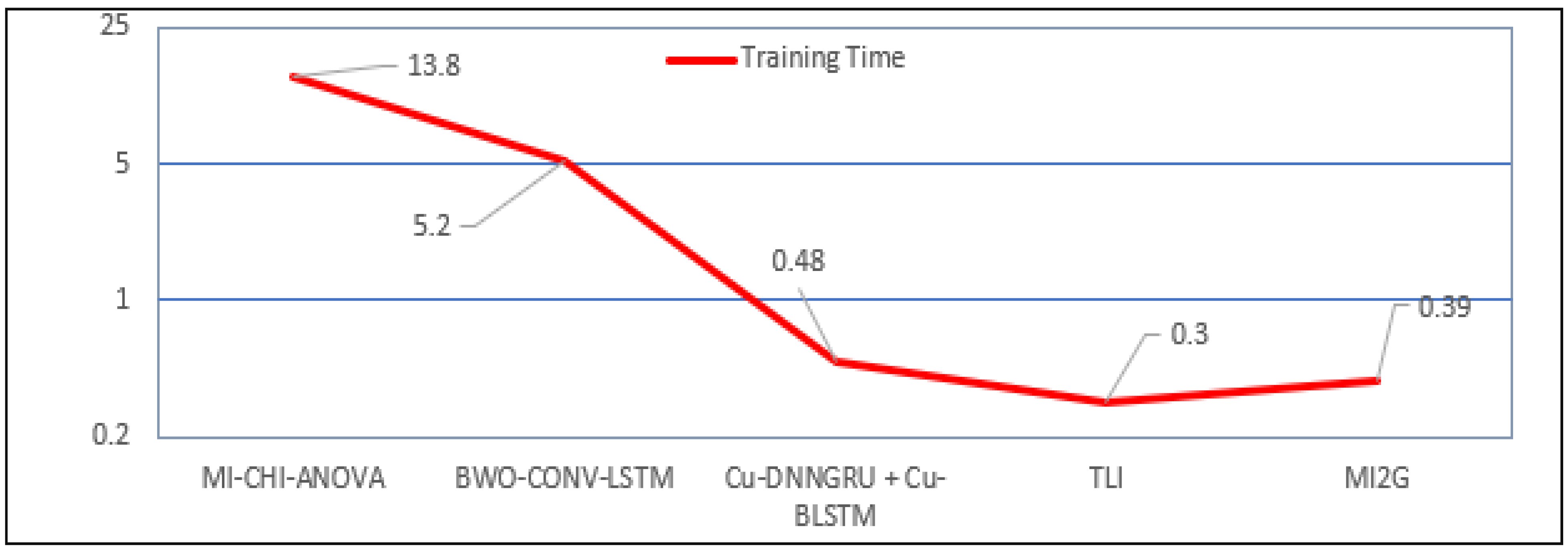Figure 13 suggests that the proposed system showed the lesser, comparable training time for the CICIDS2018 dataset, and Figure 14 suggests that the proposed system took the least time to provide comparable accuracy [56,64,65,66,67,68]. Figure 11, Figure 12, Figure 13 and Figure 14 suggest that the proposed study with the MI2G algorithm provides a consistent and balanced performance with good accuracy, Precision, Recall, and F1-Score [69,70,71] in lesser time and computational cost involved compared to previously published studies which seem to be inclined towards one parameter, leading to unbalanced results.

7. Conclusions

This research proposes a hybrid feature-selection technique using the concept of information theory for ML-based IDS to extract the relevant and essential features. The new feature selection technique, MI2G, selects the features that show high mutual information with the label and high information gain. The mutual information suggests the statistical dependence of the label on the feature, and information gain indicates the feature that contributes to the randomness in the dataset. The feature selected using the MI2G technique not only reduced the training time (in a range of 30–60%) but also boosted the accuracy (in a range of 2.7–5.1%) of the ML algorithms such as LR, LDA, NB, DT, RF, SVM, and GBM.

The DT classifier performed consistently better on all parameters than other ML classifiers. DT was able to classify the attacks with an accuracy of 99.5% and was also able to classify the attacks with similar Precision and Recall in a training time of 0.39 s. The high accuracy, Precision, and inadequate training or test time confirm that features selected using the MI2G are highly relevant and essential. Hence, this study proposes an IDS system using the MI2G feature selection technique. DT should be used for IoT systems with low computational power and more susceptible to cyber-attacks.

The IDS system proposed in this study showed better or comparable accuracy and precision than the latest studies on various datasets, such as CICIDS18 and UNSWNB15.

The authors plan to apply the proposed IDS and feature selection techniques to classify the attacks on cell phone towers in harsh locations and environments, which often have low computational power and cater to a massive amount of data. Similarly, the proposed IDS and feature selection technique for the Internet of Medical Things (IoMT) and Internet of Vehicles (IoV) prevent cyber-attacks and enable them to make decisions accurately, precisely, quickly, and locally.