
Estimate of the Biological Dose in Hadrontherapy Using GATE


 , , and
Abstract
:Simple Summary
Abstract
1. Introduction
2. Materials and Methods
2.1. Cell Survival Predictions Using mMKM and NanOx Models for Monoenergetic Ions
2.1.1. NanOx Parameters for HSG Cell Line
2.1.2. mMKM Parameters for HSG Cell Line
2.2. Prediction of Biological Dose, RBE and Cell Survivals for Spread out Bragg Peaks (SOBP)
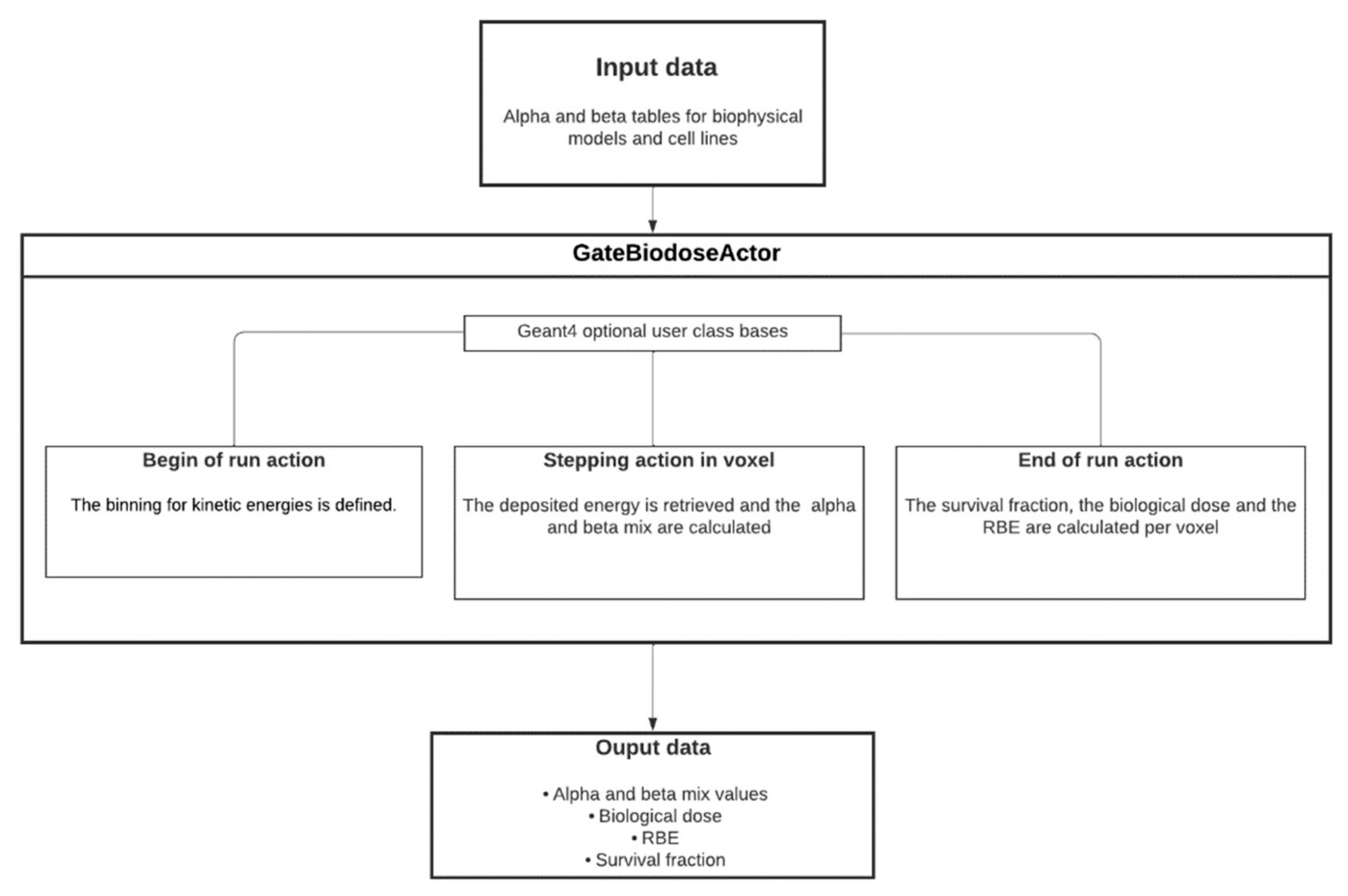
2.3. BioDoseActor Algorithm
2.4. HIBMC 320 MeV/u Carbon Ion Beam Line
3. Results
3.1. Cell Survival Predictions Using mMKM and NanOx Models
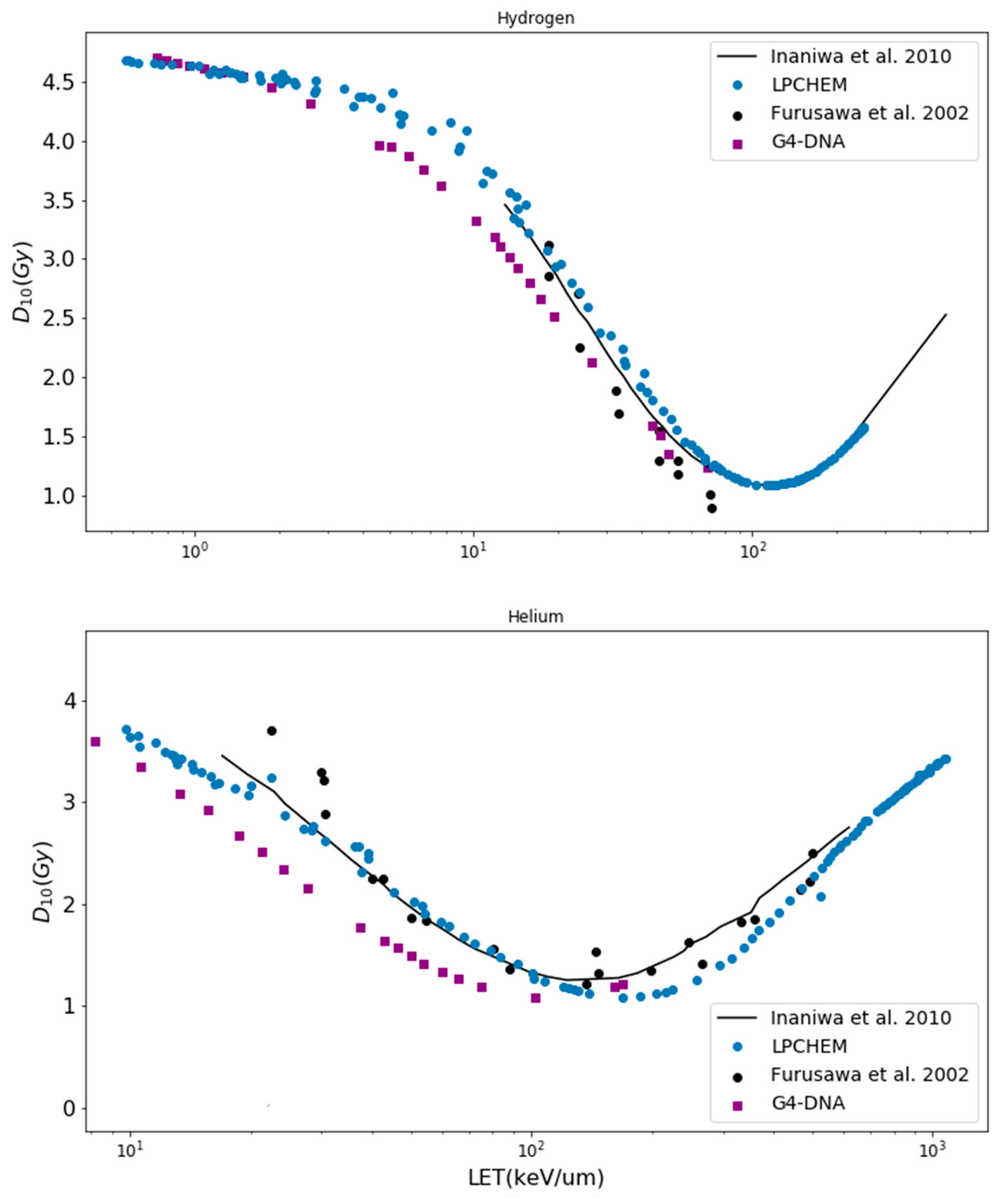
3.1.1. and D10 Values
3.1.2. Predictions of α Values as a Function of LET
- Concerning carbon ions, α values reproduced the PIDE experimental data trend for all authors;
- Concerning helium ions, α values calculated with the NanOx model were in close agreement with the PIDE experimental data. mMKM predictions from Russo et al. [31] and Chen et al. [33] resulted in close predictions except between 50 and 70 keV/μm. Higher discrepancies were observed between Geant4-DNA and PIDE experimental data;
- Concerning hydrogen ions, there were no experimental data nor predictions available in the literature. mMKM predictions, calculated with either LPCHEM or Geant4-DNA, and the NanOx model predictions, led to close results up to 25 keV/μm. For higher LET values, the NanOx model resulted in higher values than mMKM;
- Concerning oxygen ions, there were no experimental data nor predictions available in the literature. NanOx and mMKM models using LPCHEM resulted in close α values.

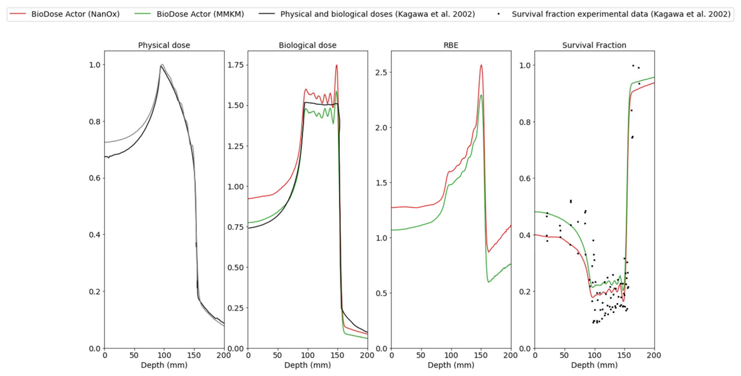
3.2. Cell Survival Fractions, Biological Doses and RBE for HIBMC 320 MeV/u Carbon-Ion Beam Line
4. Discussion
4.1. Validation of the mMKM Input Parameters for HSG Cell Line
4.2. Comparison of α Values Estimated with NanOx and mMKM Using LPCHEM and Geant4-DNA
4.3. Estimate of Cell Survival Fractions, Biological Doses and RBE for Carbon and Helium Beam Lines
5. Conclusions
Author Contributions
Funding
Institutional Review Board Statement
Informed Consent Statement
Data Availability Statement
Acknowledgments
Conflicts of Interest
Appendix A

| HYDROGEN | |||||
| E (MeV/n) | α (Gy−1) | β (Gy−2) | E (MeV/n) | α (Gy−1) | β (Gy−2) |
| 0.1 | 3.52785 | 0.0586794 | 4.25 | 0.436973 | 0.0635334 |
| 0.125 | 3.58379 | 0.0219491 | 4.25 | 0.425273 | 0.0644498 |
| 0.15 | 3.64192 | 0.0977552 | 5 | 0.420139 | 0.0625937 |
| 0.175 | 3.64134 | 0.045627 | 6 | 0.406463 | 0.0625907 |
| 0.2 | 3.59205 | 0.0522845 | 7 | 0.389055 | 0.0639294 |
| 0.225 | 3.48742 | 0.0763334 | 7.5 | 0.390886 | 0.0518132 |
| 0.25 | 3.38711 | 0.0486352 | 8 | 0.377757 | 0.0648603 |
| 0.275 | 3.23556 | 0.0140717 | 9 | 0.380409 | 0.0416042 |
| 0.3 | 3.10038 | 0.0564686 | 10 | 0.375543 | 0.0629273 |
| 0.325 | 2.92819 | 0.0736448 | 13 | 0.36375 | 0.0637803 |
| 0.35 | 2.74536 | 0.0440922 | 14 | 0.355133 | 0.0663663 |
| 0.375 | 2.64766 | 0.068873 | 14.5 | 0.363962 | 0.039987 |
| 0.4 | 2.50822 | 0.0519665 | 15 | 0.36261 | 0.0653386 |
| 0.425 | 2.35826 | 0.0598118 | 16 | 0.36199 | 0.0194867 |
| 0.45 | 2.24049 | 0.0523686 | 17 | 0.358723 | 0.0634626 |
| 0.475 | 2.11282 | 0.0327819 | 18.5 | 0.354093 | 0.0679557 |
| 0.5 | 2.00902 | 0.0619912 | 20 | 0.361473 | 0.0655274 |
| 0.525 | 1.90411 | 0.048899 | 22.5 | 0.349285 | 0.0663717 |
| 0.55 | 1.81201 | 0.03943 | 25 | 0.348734 | 0.0648933 |
| 0.6 | 1.64405 | 0.0482093 | 30 | 0.340981 | 0.0686984 |
| 0.625 | 1.5553 | 0.0315918 | 35 | 0.338952 | 0.0647853 |
| 0.65 | 1.50294 | 0.0514883 | 40 | 0.33787 | 0.0675714 |
| 0.675 | 1.42643 | 0.0530718 | 42.5 | 0.336445 | 0.0712075 |
| 0.7 | 1.37338 | 0.0520192 | 45 | 0.344386 | 0.0727018 |
| 0.725 | 1.30831 | 0.0516787 | 50 | 0.344973 | 0.0997508 |
| 0.75 | 1.27779 | 0.0520332 | 60 | 0.341337 | 0.0779679 |
| 0.775 | 1.22202 | 0.0610424 | 70 | 0.330335 | 0.0788438 |
| 0.8 | 1.17571 | 0.0540186 | 72.5 | 0.339633 | 0.083321 |
| 0.825 | 1.14052 | 0.0496843 | 75 | 0.341254 | 0.0831872 |
| 0.85 | 1.10919 | 0.0522072 | 80 | 0.343223 | 0.088238 |
| 0.875 | 1.07663 | 0.0538031 | 85 | 0.347429 | 0.0845721 |
| 0.9 | 1.04062 | 0.0541082 | 87.5 | 0.340158 | 0.0884021 |
| 0.925 | 1.0123 | 0.0436477 | 90 | 0.343359 | 0.089741 |
| 0.95 | 0.987964 | 0.0546012 | 100 | 0.3399 | 0.0930667 |
| 0.975 | 0.954701 | 0.052234 | 110 | 0.344508 | 0.0972525 |
| 0.9875 | 0.956628 | 0.0588447 | 115 | 0.341763 | 0.010713 |
| 1 | 0.931771 | 0.058776 | 120 | 0.33716 | 0.093344 |
| 1.25 | 0.922846 | 0.0596302 | 125 | 0.348853 | 0.096485 |
| 1.375 | 0.829386 | 0.057546 | 130 | 0.348952 | 0.0958178 |
| 1.4375 | 0.811162 | 0.0635889 | 132.5 | 0.342216 | 0.108084 |
| 1.5 | 0.77844 | 0.0576283 | 135 | 0.339428 | 0.109774 |
| 1.5625 | 0.743542 | 0.0617835 | 140 | 0.337172 | 0.0978914 |
| 1.625 | 0.724542 | 0.0590762 | 160 | 0.345544 | 0.101325 |
| 1.6875 | 0.705097 | 0.0629384 | 165 | 0.341937 | 0.0939792 |
| 1.75 | 0.690471 | 0.0610498 | 170 | 0.351141 | 0.0839463 |
| 1.875 | 0.657967 | 0.0689717 | 175 | 0.346595 | 0.0956681 |
| 2 | 0.630247 | 0.0609551 | 180 | 0.331431 | 0.100256 |
| 2.125 | 0.59985 | 0.0558018 | 190 | 0.334884 | 0.104186 |
| 2.25 | 0.576881 | 0.0605689 | 200 | 0.338724 | 0.105441 |
| 2.375 | 0.560703 | 0.0620355 | 212.5 | 0.333464 | 0.094867 |
| 2.5 | 0.548153 | 0.0558827 | 225 | 0.33002 | 0.129717 |
| 2.75 | 0.521374 | 0.0553158 | 237.5 | 0.342825 | 0.0705913 |
| 3 | 0.49762 | 0.0574269 | 250 | 0.346535 | 0.109787 |
| 3.25 | 0.487405 | 0.0658839 | 275 | 0.339406 | 0.0998982 |
| 3.5 | 0.467097 | 0.0576851 | 300 | 0.339219 | 0.108748 |
| 3.875 | 0.459079 | 0.0697264 | |||
| HELIUM | |||||
| E (MeV/n) | α (Gy−1) | β (Gy−2) | E (MeV/n) | α (Gy−1) | β (Gy−2) |
| 0.1 | 1.35471 | 0.0207273 | 4.625 | 0.913462 | 0.074134 |
| 0.115 | 1.34943 | 0.068132 | 4.8 | 0.894276 | 0.0399684 |
| 0.125 | 1.36143 | 0.0561437 | 5 | 0.845962 | 0.0545597 |
| 0.135 | 1.36702 | 0.0479669 | 5.5 | 0.788932 | 0.0548308 |
| 0.15 | 1.40449 | 0.0523761 | 6 | 0.729322 | 0.0589305 |
| 0.175 | 1.46176 | 0.0186978 | 7 | 0.65191 | 0.0584992 |
| 0.2 | 1.52903 | 0.0422706 | 7.5 | 0.618191 | 0.0546201 |
| 0.225 | 1.54966 | 0.0685532 | 8 | 0.594936 | 0.0590312 |
| 0.25 | 1.55482 | 0.0423817 | 9 | 0.552776 | 0.0556349 |
| 0.275 | 1.62378 | 0.0624645 | 9.5 | 0.537816 | 0.0270089 |
| 0.3 | 1.69296 | 0.0560868 | 10 | 0.521669 | 0.0646037 |
| 0.325 | 1.75868 | 0.0827488 | 12 | 0.492294 | 0.0631951 |
| 0.35 | 1.82571 | 0.09662 | 13 | 0.471319 | 0.0600745 |
| 0.375 | 1.89151 | 0.0417015 | 14 | 0.457 | 0.0540569 |
| 0.4 | 1.95804 | 0.0406013 | 14.5 | 0.454425 | 0.0647896 |
| 0.425 | 2.01788 | 0.0406869 | 15 | 0.447441 | 0.0639881 |
| 0.45 | 2.07856 | 0.0427398 | 16 | 0.442108 | 0.0585427 |
| 0.475 | 2.13803 | 0.0509513 | 17 | 0.427663 | 0.054866 |
| 0.5 | 2.19514 | 0.0360138 | 18.5 | 0.416323 | 0.0629227 |
| 0.525 | 2.24906 | 0.0560736 | 20 | 0.408267 | 0.0635374 |
| 0.55 | 2.30165 | 0.0719733 | 22.5 | 0.405099 | 0.0675533 |
| 0.56 | 2.31162 | 0.0589844 | 25 | 0.390136 | 0.0661453 |
| 0.575 | 2.35233 | 0.0283324 | 30 | 0.377674 | 0.0652145 |
| 0.58 | 2.3359 | 0.0610067 | 35 | 0.375329 | 0.0698207 |
| 0.6 | 2.24179 | 0.0365905 | 37.5 | 0.376945 | 0.068874 |
| 0.625 | 2.27969 | 0.048764 | 40 | 0.370289 | 0.0662104 |
| 0.65 | 2.32832 | 0.0571975 | 42.5 | 0.372768 | 0.0683548 |
| 0.675 | 2.36932 | 0.0582657 | 45 | 0.364365 | 0.0703231 |
| 0.7 | 2.40823 | 0.0107764 | 50 | 0.364275 | 0.0681571 |
| 0.725 | 2.44624 | 0.0803496 | 60 | 0.355372 | 0.0747071 |
| 0.75 | 2.47837 | 0.0209884 | 65 | 0.355306 | 0.0760348 |
| 0.775 | 2.51364 | 0.0847122 | 70 | 0.357653 | 0.0778917 |
| 0.8 | 2.54292 | 0.0519947 | 72.5 | 0.351378 | 0.0813151 |
| 0.825 | 2.57208 | 0.0609218 | 75 | 0.354749 | 0.0843505 |
| 0.85 | 2.59087 | 0.0639041 | 80 | 0.356145 | 0.0820511 |
| 0.875 | 2.61384 | 0.0825088 | 85 | 0.351307 | 0.087815 |
| 0.9 | 2.64201 | 0.0602317 | 87.5 | 0.359332 | 0.0900896 |
| 0.925 | 2.65902 | 0.0399342 | 90 | 0.353549 | 0.0857066 |
| 0.95 | 2.67573 | 0.0100122 | 100 | 0.352662 | 0.0869735 |
| 0.975 | 2.68649 | 0.0900614 | 110 | 0.350016 | 0.0897816 |
| 1 | 2.69945 | 0.0460438 | 120 | 0.352662 | 0.0924707 |
| 1.125 | 2.72759 | 0.0649546 | 130 | 0.349242 | 0.0993062 |
| 1.25 | 2.68623 | 0.0592119 | 132.5 | 0.350188 | 0.0977779 |
| 1.3125 | 2.67842 | 0.0437095 | 135 | 0.351315 | 0.101791 |
| 1.375 | 2.72147 | 0.0511202 | 140 | 0.351914 | 0.0996269 |
| 1.4375 | 2.6023 | 0.0481748 | 160 | 0.352059 | 0.103381 |
| 1.5 | 2.55898 | 0.0135152 | 165 | 0.348055 | 0.108882 |
| 1.5625 | 2.51015 | 0.0251847 | 170 | 0.349539 | 0.104125 |
| 1.625 | 2.51876 | 0.0820981 | 175 | 0.349366 | 0.097993 |
| 1.6875 | 2.40387 | 0.0796317 | 180 | 0.350419 | 0.104505 |
| 1.75 | 2.349 | 0.0442119 | 185 | 0.346769 | 0.107044 |
| 1.8 | 2.30672 | 0.0467401 | 190 | 0.342395 | 0.0732676 |
| 1.875 | 2.28272 | 0.0412346 | 195 | 0.349724 | 0.100912 |
| 1.9 | 2.23023 | 0.0968624 | 200 | 0.346889 | 0.116881 |
| 2 | 2.12334 | 0.0421089 | 212.5 | 0.348807 | 0.116918 |
| 2.125 | 2.05126 | 0.0369635 | 225 | 0.347231 | 0.0997025 |
| 2.25 | 1.91357 | 0.0728045 | 237.5 | 0.353986 | 0.110258 |
| 2.375 | 1.82345 | 0.0653356 | 250 | 0.34613 | 0.112309 |
| 2.5 | 1.73184 | 0.0416488 | 275 | 0.34762 | 0.107218 |
| 2.75 | 1.562 | 0.0705918 | 300 | 0.347978 | 0.101295 |
| 3 | 1.43353 | 0.0454924 | 400 | 0.344634 | 0.102051 |
| 3.25 | 1.31698 | 0.0449153 | 500 | 0.34295 | 0.109641 |
| 3.5 | 1.21521 | 0.0409911 | 600 | 0.345637 | 0.10687 |
| 3.75 | 1.13259 | 0.0515363 | 700 | 0.342868 | 0.115623 |
| 3.875 | 1.09196 | 0.0562185 | 800 | 0.341284 | 0.0974119 |
| 4.25 | 0.99491 | 0.0515848 | 900 | 0.3453 | 0.103232 |
| 1000 | 0.340597 | 0.103002 | |||
| CARBON | |||||
| E (MeV/n) | α (Gy−1) | β (Gy−2) | E (MeV/n) | α (Gy−1) | β (Gy−2) |
| 0.1 | 0.554922 | 0.0174572 | 4.625 | 1.37202 | 0.0533761 |
| 0.15 | 0.507327 | 0.0501012 | 5 | 1.41833 | 0.0934593 |
| 0.175 | 0.496762 | 0.0185161 | 6 | 1.53289 | 0.0576861 |
| 0.2 | 0.498712 | 0.0128507 | 7 | 1.6441 | 0.0352824 |
| 0.225 | 0.507064 | 0.0398217 | 7.5 | 1.6905 | 0.0484951 |
| 0.25 | 0.517163 | 0.0321235 | 8 | 1.73733 | 0.0206558 |
| 0.275 | 0.524741 | 0.028797 | 9 | 1.81111 | 0.0270153 |
| 0.3 | 0.527277 | 0.024745 | 10 | 1.86519 | 0.0145637 |
| 0.35 | 0.562364 | 0.0325134 | 13 | 1.9013 | 0.0735242 |
| 0.375 | 0.581553 | 0.04897 | 14 | 1.88 | 0.0524471 |
| 0.4 | 0.600128 | 0.022651 | 14.5 | 1.86598 | 0.0753743 |
| 0.45 | 0.63878 | 0.0493113 | 15 | 1.84803 | 0.0247954 |
| 0.475 | 0.658849 | 0.0709208 | 16 | 1.80727 | 0.0386726 |
| 0.5 | 0.678314 | 0.0311766 | 17 | 1.75589 | 0.127889 |
| 0.525 | 0.651331 | 0.0378454 | 18.5 | 1.6866 | 0.0289437 |
| 0.53 | 0.654257 | 0.0387549 | 20 | 1.59615 | 0.0269112 |
| 0.55 | 0.668569 | 0.0323383 | 22.5 | 1.46482 | 0.02547 |
| 0.575 | 0.685794 | 0.0958369 | 25 | 1.3439 | 0.0377534 |
| 0.6 | 0.698747 | 0.0925473 | 27 | 1.25757 | 0.0699588 |
| 0.625 | 0.71445 | 0.0123321 | 30 | 1.14384 | 0.063285 |
| 0.65 | 0.729095 | 0.018834 | 32 | 1.08349 | 0.0503975 |
| 0.675 | 0.743807 | 0.033274 | 35 | 0.995382 | 0.0563748 |
| 0.7 | 0.757473 | 0.032298 | 37.5 | 0.937827 | 0.0468086 |
| 0.725 | 0.771899 | 0.029902 | 40 | 0.883756 | 0.0536156 |
| 0.75 | 0.7715 | 0.0258204 | 42.5 | 0.843352 | 0.06574 |
| 0.775 | 0.780193 | 0.0222819 | 45 | 0.806053 | 0.060595 |
| 0.8 | 0.792595 | 0.0115817 | 50 | 0.742661 | 0.0559711 |
| 0.825 | 0.804823 | 0.0254497 | 60 | 0.656602 | 0.0738968 |
| 0.85 | 0.818199 | 0.0192019 | 65 | 0.622154 | 0.0275371 |
| 0.875 | 0.828681 | 0.019282 | 70 | 0.587718 | 0.0599057 |
| 0.9 | 0.838734 | 0.0572171 | 72.5 | 0.581034 | 0.0643803 |
| 0.925 | 0.847032 | 0.0501417 | 75 | 0.579367 | 0.0263508 |
| 0.95 | 0.857266 | 0.0462406 | 80 | 0.570936 | 0.0643563 |
| 0.975 | 0.868805 | 0.0614917 | 85 | 0.557118 | 0.0420902 |
| 0.9875 | 0.875099 | 0.0422347 | 87.5 | 0.55305 | 0.064244 |
| 1 | 0.875006 | 0.08374 | 90 | 0.549996 | 0.060972 |
| 1.125 | 0.918784 | 0.0602353 | 100 | 0.529454 | 0.044553 |
| 1.25 | 0.920182 | 0.0925326 | 110 | 0.514361 | 0.0641633 |
| 1.3125 | 0.937178 | 0.0795297 | 120 | 0.500774 | 0.0656887 |
| 1.375 | 0.949605 | 0.0347631 | 130 | 0.490693 | 0.0572786 |
| 1.4375 | 0.964492 | 0.0309748 | 132.5 | 0.486477 | 0.0687478 |
| 1.5 | 0.981289 | 0.0190316 | 135 | 0.484113 | 0.0336333 |
| 1.5625 | 0.993225 | 0.0224706 | 140 | 0.479973 | 0.0652569 |
| 1.625 | 1.00636 | 0.0147146 | 150 | 0.471674 | 0.0623355 |
| 1.6875 | 1.0206 | 0.039587 | 160 | 0.464491 | 0.0678329 |
| 1.75 | 1.0308 | 0.0626443 | 165 | 0.461521 | 0.0694929 |
| 1.875 | 1.03536 | 0.0595288 | 175 | 0.455044 | 0.0702457 |
| 2 | 1.03757 | 0.140597 | 180 | 0.454354 | 0.0690091 |
| 2.125 | 1.05661 | 0.0580031 | 185 | 0.450706 | 0.0807745 |
| 2.25 | 1.07951 | 0.047584 | 190 | 0.446442 | 0.0477704 |
| 2.5 | 1.11612 | 0.0134392 | 195 | 0.445182 | 0.0765487 |
| 2.75 | 1.15096 | 0.0417291 | 200 | 0.443174 | 0.075495 |
| 3 | 1.18637 | 0.0549517 | 212.5 | 0.436772 | 0.0750927 |
| 3.25 | 1.2192 | 0.0958209 | 225 | 0.432475 | 0.0477424 |
| 3.5 | 1.25362 | 0.034796 | 237.5 | 0.429575 | 0.0770921 |
| 3.875 | 1.27999 | 0.0602744 | 250 | 0.428672 | 0.0863672 |
| 4.25 | 1.3268 | 0.0283756 | 275 | 0.419821 | 0.0642036 |
| 300 | 0.414074 | 0.0833777 | |||
| OXYGEN | |||||
| E (MeV/n) | α (Gy−1) | β (Gy−2) | E (MeV/n) | α (Gy−1) | β (Gy−2) |
| 0.1 | 0.413736 | 0.0142512 | 6 | 1.09991 | 0.0179879 |
| 0.2 | 0.389411 | 0.0289218 | 7 | 1.17086 | 0.0553748 |
| 0.25 | 0.390787 | 0.0132718 | 8 | 1.23791 | 0.03446 |
| 0.3 | 0.408917 | 0.0151436 | 10 | 1.36301 | 0.0780824 |
| 0.35 | 0.432501 | 0.0102363 | 13 | 1.53735 | 0.0380272 |
| 0.4 | 0.457564 | 0.0140088 | 15 | 1.63487 | 0.0208637 |
| 0.45 | 0.487057 | 0.0416276 | 20 | 1.77359 | 0.0114724 |
| 0.5 | 0.512859 | 0.029806 | 25 | 1.78011 | 0.0369413 |
| 0.55 | 0.497537 | 0.0513708 | 30 | 1.69153 | 0.0243579 |
| 0.6 | 0.519719 | 0.023812 | 40 | 1.43087 | 0.0687465 |
| 0.7 | 0.561975 | 0.0147102 | 50 | 1.20946 | 0.0680245 |
| 0.75 | 0.585803 | 0.0239479 | 60 | 1.044 | 0.0593522 |
| 0.8 | 0.608447 | 0.00467075 | 70 | 0.93624 | 0.0608797 |
| 0.85 | 0.618215 | 0.0265444 | 80 | 0.854476 | 0.0671706 |
| 0.9 | 0.636862 | 0.0320603 | 90 | 0.803408 | 0.0549333 |
| 0.95 | 0.65226 | 0.0291653 | 100 | 0.758682 | 0.0548792 |
| 1 | 0.670432 | 0.0378584 | 110 | 0.720772 | 0.0656161 |
| 1.25 | 0.710918 | 0.0462263 | 120 | 0.689713 | 0.0541748 |
| 1.5 | 0.7642 | 0.0888616 | 130 | 0.659153 | 0.0666365 |
| 1.75 | 0.794974 | 0.0780676 | 140 | 0.641074 | 0.0580988 |
| 2.25 | 0.836185 | 0.0696362 | 150 | 0.621408 | 0.0605031 |
| 2.5 | 0.864835 | 0.0403956 | 160 | 0.602909 | 0.0606604 |
| 2.75 | 0.880924 | 0.0148689 | 180 | 0.576667 | 0.0703917 |
| 3 | 0.894613 | 0.00887251 | 200 | 0.556955 | 0.0680523 |
| 3.5 | 0.941321 | 0.0402146 | 250 | 0.517284 | 0.0828523 |
| 5 | 1.04036 | 0.0320689 | 300 | 0.493476 | 0.0861731 |
| 350 | 0.47441 | 0.0914356 | |||
Appendix B
| HYDROGEN | |||||
| E (MeV/n) | α (Gy−1) | β (Gy−2) | E (MeV/n) | α (Gy−1) | β (Gy−2) |
| 0.1 | 1.76015784 | 0.0615 | 4.25 | 0.41269852 | 0.0615 |
| 0.125 | 1.90316891 | 0.0615 | 4.625 | 0.39792158 | 0.0615 |
| 0.15 | 1.85167715 | 0.0615 | 5 | 0.37526441 | 0.0615 |
| 0.175 | 1.79620928 | 0.0615 | 6 | 0.3465522 | 0.0615 |
| 0.2 | 1.72047753 | 0.0615 | 7 | 0.32547431 | 0.0615 |
| 0.225 | 1.686197 | 0.0615 | 7.5 | 0.31677023 | 0.0615 |
| 0.25 | 1.63496363 | 0.0615 | 8 | 0.31103573 | 0.0615 |
| 0.275 | 1.55673265 | 0.0615 | 9 | 0.30400634 | 0.0615 |
| 0.3 | 1.50465213 | 0.0615 | 10 | 0.29759482 | 0.0615 |
| 0.325 | 1.45851417 | 0.0615 | 13 | 0.27563387 | 0.0615 |
| 0.35 | 1.40890868 | 0.0615 | 14 | 0.25797535 | 0.0615 |
| 0.375 | 1.37158627 | 0.0615 | 14.5 | 0.26592402 | 0.0615 |
| 0.4 | 1.34708463 | 0.0615 | 15 | 0.2607293 | 0.0615 |
| 0.425 | 1.28856167 | 0.0615 | 16 | 0.25896092 | 0.0615 |
| 0.45 | 1.27640762 | 0.0615 | 17 | 0.2597976 | 0.0615 |
| 0.475 | 1.22548674 | 0.0615 | 18.5 | 0.24932084 | 0.0615 |
| 0.5 | 1.20290671 | 0.0615 | 20 | 0.23703403 | 0.0615 |
| 0.525 | 1.16652015 | 0.0615 | 22.5 | 0.23584525 | 0.0615 |
| 0.55 | 1.14828801 | 0.0615 | 25 | 0.24512923 | 0.0615 |
| 0.6 | 1.10455273 | 0.0615 | 30 | 0.23253512 | 0.0615 |
| 0.625 | 1.0710152 | 0.0615 | 35 | 0.22953456 | 0.0615 |
| 0.65 | 1.0442441 | 0.0615 | 40 | 0.22510101 | 0.0615 |
| 0.675 | 1.02892927 | 0.0615 | 42.5 | 0.21525845 | 0.0615 |
| 0.7 | 1.01230563 | 0.0615 | 45 | 0.21364756 | 0.0615 |
| 0.725 | 1.00993717 | 0.0615 | 50 | 0.20728247 | 0.0615 |
| 0.75 | 0.99169901 | 0.0615 | 60 | 0.21160957 | 0.0615 |
| 0.775 | 0.9504684 | 0.0615 | 70 | 0.21542632 | 0.0615 |
| 0.8 | 0.93575076 | 0.0615 | 72.5 | 0.21168926 | 0.0615 |
| 0.825 | 0.93725789 | 0.0615 | 75 | 0.21454225 | 0.0615 |
| 0.85 | 0.91940491 | 0.0615 | 80 | 0.20557802 | 0.0615 |
| 0.875 | 0.90710971 | 0.0615 | 85 | 0.20915264 | 0.0615 |
| 0.9 | 0.88489348 | 0.0615 | 87.5 | 0.21005575 | 0.0615 |
| 0.925 | 0.85892201 | 0.0615 | 90 | 0.19931656 | 0.0615 |
| 0.95 | 0.84808765 | 0.0615 | 100 | 0.20679814 | 0.0615 |
| 0.975 | 0.82971714 | 0.0615 | 110 | 0.20829383 | 0.0615 |
| 0.988 | 0.85598572 | 0.0615 | 115 | 0.20360297 | 0.0615 |
| 1 | 0.9810095 | 0.0615 | 120 | 0.20592231 | 0.0615 |
| 1.375 | 0.81205418 | 0.0615 | 125 | 0.20449326 | 0.0615 |
| 1.438 | 0.81442601 | 0.0615 | 130 | 0.20444967 | 0.0615 |
| 1.5 | 0.75449721 | 0.0615 | 132.5 | 0.20764789 | 0.0615 |
| 1.562 | 0.75771038 | 0.0615 | 135 | 0.20557136 | 0.0615 |
| 1.625 | 0.73026718 | 0.0615 | 140 | 0.20865446 | 0.0615 |
| 1.688 | 0.69581744 | 0.0615 | 160 | 0.2021342 | 0.0615 |
| 1.75 | 0.69183551 | 0.0615 | 165 | 0.19910029 | 0.0615 |
| 1.875 | 0.66042851 | 0.0615 | 170 | 0.20163043 | 0.0615 |
| 2 | 0.63047876 | 0.0615 | 175 | 0.20342183 | 0.0615 |
| 2.125 | 0.61644836 | 0.0615 | 180 | 0.19935637 | 0.0615 |
| 2.25 | 0.57953347 | 0.0615 | 190 | 0.19497002 | 0.0615 |
| 2.375 | 0.58510633 | 0.0615 | 200 | 0.19964379 | 0.0615 |
| 2.5 | 0.54312614 | 0.0615 | 212.5 | 0.19807176 | 0.0615 |
| 2.75 | 0.52668644 | 0.0615 | 225 | 0.1980282 | 0.0615 |
| 3 | 0.5225944 | 0.0615 | 237.5 | 0.19863153 | 0.0615 |
| 3.25 | 0.47132339 | 0.0615 | 250 | 0.20256654 | 0.0615 |
| 3.5 | 0.45446625 | 0.0615 | 275 | 0.19835696 | 0.0615 |
| 3.875 | 0.42329655 | 0.0615 | 300 | 0.19917811 | 0.0615 |
| HELIUM | |||||
| E (MeV/n) | α (Gy−1) | β (Gy−2) | E (MeV/n) | α (Gy−1) | β (Gy−2) |
| 0.1 | 1.39368254 | 0.0615 | 4.625 | 0.96230827 | 0.0615 |
| 0.115 | 1.36937733 | 0.0615 | 4.8 | 0.94225563 | 0.0615 |
| 0.125 | 1.36745112 | 0.0615 | 5 | 0.88911444 | 0.0615 |
| 0.135 | 1.36213099 | 0.0615 | 5.5 | 0.83434223 | 0.0615 |
| 0.15 | 1.38439522 | 0.0615 | 6 | 0.82117505 | 0.0615 |
| 0.175 | 1.42048374 | 0.0615 | 7 | 0.72771876 | 0.0615 |
| 0.2 | 1.47155149 | 0.0615 | 7.5 | 0.67973888 | 0.0615 |
| 0.225 | 1.51566938 | 0.0615 | 8 | 0.65120626 | 0.0615 |
| 0.25 | 1.45535665 | 0.0615 | 9 | 0.60447989 | 0.0615 |
| 0.275 | 1.51257501 | 0.0615 | 9.5 | 0.59490674 | 0.0615 |
| 0.3 | 1.56460825 | 0.0615 | 12 | 0.517091 | 0.0615 |
| 0.325 | 1.60506986 | 0.0615 | 13 | 0.49108525 | 0.0615 |
| 0.35 | 1.66200317 | 0.0615 | 14 | 0.48217333 | 0.0615 |
| 0.375 | 1.70567852 | 0.0615 | 14.5 | 0.45355589 | 0.0615 |
| 0.4 | 1.75101482 | 0.0615 | 15 | 0.4603493 | 0.0615 |
| 0.425 | 1.78517233 | 0.0615 | 16 | 0.43637705 | 0.0615 |
| 0.45 | 1.82903515 | 0.0615 | 17 | 0.42769368 | 0.0615 |
| 0.475 | 1.86894901 | 0.0615 | 18.5 | 0.40850354 | 0.0615 |
| 0.5 | 1.89593537 | 0.0615 | 20 | 0.38354342 | 0.0615 |
| 0.525 | 1.91584789 | 0.0615 | 22.5 | 0.39052976 | 0.0615 |
| 0.55 | 1.9416978 | 0.0615 | 25 | 0.34625961 | 0.0615 |
| 0.56 | 1.95247026 | 0.0615 | 30 | 0.34060395 | 0.0615 |
| 0.575 | 1.96519554 | 0.0615 | 35 | 0.31125112 | 0.0615 |
| 0.58 | 1.97270031 | 0.0615 | 37.5 | 0.31120437 | 0.0615 |
| 0.6 | 1.90338008 | 0.0615 | 40 | 0.30110398 | 0.0615 |
| 0.625 | 1.93381438 | 0.0615 | 42.5 | 0.29806927 | 0.0615 |
| 0.65 | 1.94856927 | 0.0615 | 45 | 0.28731212 | 0.0615 |
| 0.675 | 1.96447665 | 0.0615 | 50 | 0.28434712 | 0.0615 |
| 0.7 | 1.99257377 | 0.0615 | 60 | 0.27235922 | 0.0615 |
| 0.725 | 2.004059 | 0.0615 | 65 | 0.27475892 | 0.0615 |
| 0.75 | 2.0092631 | 0.0615 | 70 | 0.25924287 | 0.0615 |
| 0.775 | 2.02168365 | 0.0615 | 72.5 | 0.25075129 | 0.0615 |
| 0.8 | 2.03352762 | 0.0615 | 75 | 0.25857623 | 0.0615 |
| 0.825 | 2.03364266 | 0.0615 | 80 | 0.25831101 | 0.0615 |
| 0.85 | 2.04461617 | 0.0615 | 85 | 0.2523552 | 0.0615 |
| 0.875 | 2.04794839 | 0.0615 | 87.5 | 0.23523516 | 0.0615 |
| 0.9 | 2.04944316 | 0.0615 | 90 | 0.24796673 | 0.0615 |
| 0.925 | 2.05383802 | 0.0615 | 100 | 0.24530574 | 0.0615 |
| 0.95 | 2.05227089 | 0.0615 | 110 | 0.23886659 | 0.0615 |
| 0.975 | 2.05360573 | 0.0615 | 120 | 0.23670685 | 0.0615 |
| 1 | 2.04932288 | 0.0615 | 130 | 0.23381593 | 0.0615 |
| 1.125 | 2.03431604 | 0.0615 | 132.5 | 0.23330326 | 0.0615 |
| 1.25 | 2.00341284 | 0.0615 | 135 | 0.22587891 | 0.0615 |
| 1.312 | 1.97632077 | 0.0615 | 140 | 0.22961596 | 0.0615 |
| 1.375 | 1.94453497 | 0.0615 | 160 | 0.22902871 | 0.0615 |
| 1.438 | 1.93463072 | 0.0615 | 165 | 0.23033065 | 0.0615 |
| 1.5 | 1.91692309 | 0.0615 | 170 | 0.22880151 | 0.0615 |
| 1.562 | 1.88227096 | 0.0615 | 175 | 0.22281551 | 0.0615 |
| 1.625 | 1.82822213 | 0.0615 | 180 | 0.22562653 | 0.0615 |
| 1.688 | 1.81990989 | 0.0615 | 185 | 0.2232301 | 0.0615 |
| 1.75 | 1.79166858 | 0.0615 | 190 | 0.21677319 | 0.0615 |
| 1.8 | 1.76094575 | 0.0615 | 195 | 0.22151075 | 0.0615 |
| 1.875 | 1.75294194 | 0.0615 | 200 | 0.22526867 | 0.0615 |
| 1.9 | 1.69542062 | 0.0615 | 212.5 | 0.2183769 | 0.0615 |
| 2 | 1.67302649 | 0.0615 | 225 | 0.22302907 | 0.0615 |
| 2.125 | 1.60603852 | 0.0615 | 237.5 | 0.2219778 | 0.0615 |
| 2.25 | 1.57159 | 0.0615 | 250 | 0.21148815 | 0.0615 |
| 2.375 | 1.5227767 | 0.0615 | 275 | 0.22256361 | 0.0615 |
| 2.5 | 1.49062651 | 0.0615 | 300 | 0.2120016 | 0.0615 |
| 2.75 | 1.37790739 | 0.0615 | 400 | 0.21014623 | 0.0615 |
| 3 | 1.29101377 | 0.0615 | 500 | 0.21069392 | 0.0615 |
| 3.25 | 1.23449549 | 0.0615 | 600 | 0.20814372 | 0.0615 |
| 3.5 | 1.16275574 | 0.0615 | 700 | 0.20445455 | 0.0615 |
| 3.75 | 1.11019208 | 0.0615 | 800 | 0.20849856 | 0.0615 |
| 3.875 | 1.07576636 | 0.0615 | 900 | 0.20332779 | 0.0615 |
| 4.25 | 1.00479394 | 0.0615 | 1000 | 0.20570698 | 0.0615 |
| CARBON | |||||
| E (MeV/n) | α (Gy−1) | β (Gy−2) | E (MeV/n) | α (Gy−1) | β (Gy−2) |
| 0.15 | 0.50339808 | 0.0615 | 5 | 1.55653422 | 0.0615 |
| 0.175 | 0.48454942 | 0.0615 | 6 | 1.75053464 | 0.0615 |
| 0.2 | 0.47487403 | 0.0615 | 7 | 1.90877459 | 0.0615 |
| 0.225 | 0.47187832 | 0.0615 | 7.5 | 1.95249266 | 0.0615 |
| 0.25 | 0.47407494 | 0.0615 | 8 | 1.99679369 | 0.0615 |
| 0.275 | 0.45992261 | 0.0615 | 9 | 2.03862693 | 0.0615 |
| 0.3 | 0.46235642 | 0.0615 | 10 | 2.05601166 | 0.0615 |
| 0.35 | 0.47192496 | 0.0615 | 13 | 1.97305347 | 0.0615 |
| 0.375 | 0.47813642 | 0.0615 | 14 | 1.94262411 | 0.0615 |
| 0.4 | 0.48505401 | 0.0615 | 14.5 | 1.90610348 | 0.0615 |
| 0.45 | 0.49879305 | 0.0615 | 15 | 1.89554533 | 0.0615 |
| 0.475 | 0.50483791 | 0.0615 | 16 | 1.85562239 | 0.0615 |
| 0.5 | 0.51322218 | 0.0615 | 17 | 1.77657221 | 0.0615 |
| 0.525 | 0.49146793 | 0.0615 | 18.5 | 1.73405714 | 0.0615 |
| 0.53 | 0.49445111 | 0.0615 | 20 | 1.66676365 | 0.0615 |
| 0.55 | 0.49573957 | 0.0615 | 22.5 | 1.54318579 | 0.0615 |
| 0.575 | 0.50445866 | 0.0615 | 25 | 1.46078637 | 0.0615 |
| 0.6 | 0.51250679 | 0.0615 | 27 | 1.40127589 | 0.0615 |
| 0.625 | 0.51767073 | 0.0615 | 30 | 1.32642616 | 0.0615 |
| 0.65 | 0.5256997 | 0.0615 | 32 | 1.27113082 | 0.0615 |
| 0.675 | 0.53160257 | 0.0615 | 35 | 1.1848265 | 0.0615 |
| 0.7 | 0.53863325 | 0.0615 | 37.5 | 1.14827529 | 0.0615 |
| 0.725 | 0.54617082 | 0.0615 | 40 | 1.09587716 | 0.0615 |
| 0.75 | 0.54341952 | 0.0615 | 42.5 | 1.03951646 | 0.0615 |
| 0.775 | 0.54739658 | 0.0615 | 45 | 1.01144134 | 0.0615 |
| 0.8 | 0.55725082 | 0.0615 | 50 | 0.95704141 | 0.0615 |
| 0.825 | 0.56183319 | 0.0615 | 60 | 0.84947386 | 0.0615 |
| 0.85 | 0.56804995 | 0.0615 | 65 | 0.79309164 | 0.0615 |
| 0.875 | 0.57653972 | 0.0615 | 70 | 0.76869037 | 0.0615 |
| 0.9 | 0.58180655 | 0.0615 | 72.5 | 0.74023123 | 0.0615 |
| 0.925 | 0.58825069 | 0.0615 | 75 | 0.7394691 | 0.0615 |
| 0.95 | 0.59650123 | 0.0615 | 80 | 0.7154438 | 0.0615 |
| 0.975 | 0.60167595 | 0.0615 | 85 | 0.67492106 | 0.0615 |
| 0.988 | 0.60524041 | 0.0615 | 87.5 | 0.6745586 | 0.0615 |
| 1 | 0.6126607 | 0.0615 | 90 | 0.66200055 | 0.0615 |
| 1.125 | 0.64546276 | 0.0615 | 100 | 0.62537666 | 0.0615 |
| 1.25 | 0.64506518 | 0.0615 | 110 | 0.51090028 | 0.0615 |
| 1.312 | 0.66343661 | 0.0615 | 120 | 0.56221711 | 0.0615 |
| 1.375 | 0.6801614 | 0.0615 | 130 | 0.54273609 | 0.0615 |
| 1.438 | 0.69527217 | 0.0615 | 132.5 | 0.53486851 | 0.0615 |
| 1.5 | 0.71570436 | 0.0615 | 135 | 0.53097809 | 0.0615 |
| 1.562 | 0.7343878 | 0.0615 | 140 | 0.52415145 | 0.0615 |
| 1.625 | 0.74580065 | 0.0615 | 150 | 0.50843461 | 0.0615 |
| 1.688 | 0.76131236 | 0.0615 | 160 | 0.49663483 | 0.0615 |
| 1.75 | 0.78269442 | 0.0615 | 165 | 0.48895603 | 0.0615 |
| 1.875 | 0.80061062 | 0.0615 | 175 | 0.47546677 | 0.0615 |
| 2 | 0.83450504 | 0.0615 | 180 | 0.47380211 | 0.0615 |
| 2.125 | 0.8360636 | 0.0615 | 185 | 0.46439192 | 0.0615 |
| 2.25 | 0.87478362 | 0.0615 | 190 | 0.4597621 | 0.0615 |
| 2.5 | 0.93848816 | 0.0615 | 195 | 0.45408332 | 0.0615 |
| 2.75 | 1.0071553 | 0.0615 | 200 | 0.45227578 | 0.0615 |
| 3 | 1.08229543 | 0.0615 | 212.5 | 0.44305794 | 0.0615 |
| 3.25 | 1.15264005 | 0.0615 | 225 | 0.43045946 | 0.0615 |
| 3.5 | 1.21718809 | 0.0615 | 237.5 | 0.42182226 | 0.0615 |
| 3.875 | 1.28441299 | 0.0615 | 250 | 0.40828412 | 0.0615 |
| 4.25 | 1.36850829 | 0.0615 | 275 | 0.40622332 | 0.0615 |
| 4.625 | 1.48784096 | 0.0615 | 300 | 0.39136842 | 0.0615 |
| OXYGEN | |||||
| E (MeV/n) | α (Gy−1) | β (Gy−2) | E (MeV/n) | α (Gy−1) | β (Gy−2) |
| 0.1 | 0.57683641 | 0.0615 | 40 | 1.61813083 | 0.0615 |
| 0.2 | 0.39461372 | 0.0615 | 50 | 1.41288483 | 0.0615 |
| 0.25 | 0.38549096 | 0.0615 | 60 | 1.2769869 | 0.0615 |
| 0.3 | 0.38420183 | 0.0615 | 70 | 1.1465992 | 0.0615 |
| 0.35 | 0.38874355 | 0.0615 | 80 | 1.0769192 | 0.0615 |
| 0.4 | 0.39431564 | 0.0615 | 90 | 0.99183267 | 0.0615 |
| 0.45 | 0.40153681 | 0.0615 | 100 | 0.93563608 | 0.0615 |
| 0.5 | 0.41036818 | 0.0615 | 110 | 0.90126161 | 0.0615 |
| 0.55 | 0.39382537 | 0.0615 | 120 | 0.83897904 | 0.0615 |
| 0.6 | 0.40244051 | 0.0615 | 130 | 0.80282571 | 0.0615 |
| 0.7 | 0.41948742 | 0.0615 | 140 | 0.76208427 | 0.0615 |
| 0.75 | 0.42708322 | 0.0615 | 150 | 0.73875254 | 0.0615 |
| 0.8 | 0.43581879 | 0.0615 | 160 | 0.71921426 | 0.0615 |
| 0.85 | 0.44460969 | 0.0615 | 180 | 0.67685998 | 0.0615 |
| 0.9 | 0.45262565 | 0.0615 | 200 | 0.63836255 | 0.0615 |
| 0.95 | 0.46079407 | 0.0615 | 250 | 0.58416082 | 0.0615 |
| 1 | 0.47074632 | 0.0615 | 300 | 0.53276501 | 0.0615 |
| 1.25 | 0.5008777 | 0.0615 | 350 | 0.50905649 | 0.0615 |
| 1.5 | 0.53970912 | 0.0615 | 400 | 0.48671036 | 0.0615 |
| 1.75 | 0.57550625 | 0.0615 | 0.75 | 0.36571457 | 0.0615 |
| 2.25 | 0.63054616 | 0.0615 | 1.5 | 0.43244717 | 0.0615 |
| 2.5 | 0.662315 | 0.0615 | 1.7 | 0.45753939 | 0.0615 |
| 2.75 | 0.69868629 | 0.0615 | 2.8 | 0.55556211 | 0.0615 |
| 3 | 0.74023048 | 0.0615 | 5 | 0.73531098 | 0.0615 |
| 3.5 | 0.82502643 | 0.0615 | 7 | 0.91601311 | 0.0615 |
| 5 | 1.02532216 | 0.0615 | 8 | 1.01432123 | 0.0615 |
| 6 | 1.17652843 | 0.0615 | 10 | 1.18638951 | 0.0615 |
| 7 | 1.2918773 | 0.0615 | 13 | 1.44146401 | 0.0615 |
| 8 | 1.42043736 | 0.0615 | 15 | 1.59418043 | 0.0615 |
| 10 | 1.66855287 | 0.0615 | 80 | 1.45976032 | 0.0615 |
| 13 | 1.92005086 | 0.0615 | 85 | 1.40898716 | 0.0615 |
| 15 | 2.00085691 | 0.0615 | 90 | 1.35830835 | 0.0615 |
| 20 | 2.04557772 | 0.0615 | 95 | 1.32300946 | 0.0615 |
| 25 | 1.96074999 | 0.0615 | 100 | 1.29277276 | 0.0615 |
| 30 | 1.85318684 | 0.0615 | |||
References
- Paganetti, H. Range uncertainties in proton therapy and the role of Monte Carlo simulations. Phys. Med. Biol. 2012, 57, R99–R117. [Google Scholar] [CrossRef]
- Paganetti, H. Relative biological effectiveness (RBE) values for proton beam therapy. Variations as a function of biological endpoint, dose, and linear energy transfer. Phys. Med. Biol. 2014, 59, R419. [Google Scholar] [CrossRef]
- Karger, C.P.; Peschke, P. RBE and related modeling in carbon-ion therapy. Phys. Med. Biol. 2018, 63, 01TR02. [Google Scholar] [CrossRef]
- Paganetti, H.; Blakely, E.; Carabe-Fernandez, A.; Carlson, D.J.; Das, I.J.; Dong, L.; Grosshans, D.; Held, K.D.; Mohan, R.; Moiseenko, V.; et al. Report of the AAPM TG-256 on the relative biological effectiveness of proton beams in radiation therapy. Med. Phys. 2019, 46, e53–e78. [Google Scholar] [CrossRef] [Green Version]
- Böhlen, T.T.; Dosanjh, M.; Ferrari, A.; Gudowska, I.A.; Mairani, A. FLUKA simulations of the response of tissue-equivalent proportional counters to ion beams for applications in hadron therapy and space. Phys. Med. Biol. 2011, 56, 6545–6561. [Google Scholar] [CrossRef]
- Kramer, M.; Scholz, M. Treatment planning for heavy-ion radiotherapy: Calculation and optimization of biologically effective dose. Phys. Med. Biol. 2000, 45, 3319. [Google Scholar] [CrossRef]
- Grün, R.; Friedrich, T.; Krämer, M.; Scholz, M. Systematics of relative biological effectiveness measurements for proton radiation along the spread out Bragg peak: Experimental validation of the local effect model. Phys. Med. Biol. 2017, 62, 890. [Google Scholar] [CrossRef]
- Jan, S.; Santin, G.; Strul, D.; Staelens, S.; Assié, K.; Autret, D.; Avner, S.; Barbier, R.; Bardiès, M.; Bloomfield, P.M.; et al. GATE: A simulation toolkit for PET and SPECT. Phys. Med. Biol. 2004, 49, 4543–4561. [Google Scholar] [CrossRef]
- Jan, S.; Benoit, D.; Becheva, E.; Carlier, T.; Cassol, F.; Descourt, P.; Frisson, T.; Grevillot, L.; Guigues, L.; Maigne, L.; et al. GATE V6: A major enhancement of the GATE simulation platform enabling modelling of CT and radiotherapy. Phys. Med. Biol. 2011, 56, 881. [Google Scholar] [CrossRef]
- Sarrut, D.; Bardiès, M.; Boussion, N.; Freud, N.; Jan, S.; Létang, J.-M.; Loudos, G.; Maigne, L.; Marcatili, S.; Mauxion, T.; et al. A review of the use and potential of the GATE Monte Carlo simulation code for radiation therapy and dosimetry applications. Med. Phys. 2014, 41, 064301. [Google Scholar] [CrossRef] [Green Version]
- Winterhalter, C.; Taylor, M.; Boersma, D.; Elia, A.; Guatelli, S.; Mackay, R.; Kirkby, K.; Maigne, L.; Ivanchenko, V.; Resch, A.F.; et al. Evaluation of GATE-RTion (GATE/Geant4) Monte Carlo simulation settings for proton pencil beam scanning quality assurance. Med. Phys. 2020, 47, 5817–5828. [Google Scholar] [CrossRef] [PubMed]
- Grevillot, L.; Boersma, D.J.; Fuchs, H.; Aitkenhead, A.; Elia, A.; Bolsa, M.; Winterhalter, C.; Vidal, M.; Jan, S.; Pietrzyk, U.; et al. Technical Note: GATE-RTion: A GATE/Geant4 release for clinical applications in scanned ion beam therapy. Med. Phys. 2020, 47, 3675–3681. [Google Scholar] [CrossRef] [PubMed]
- Grevillot, L.; Boersma, D.J.; Fuchs, H.; Bolsa-Ferruz, M.; Scheuchenpflug, L.; Georg, D.; Kronreif, G.; Stock, M. The GATE-RTion/IDEAL Independent Dose Calculation System for Light Ion Beam Therapy. Front. Phys. 2021, 9, 424. [Google Scholar] [CrossRef]
- Hawkins, R. A microdosimetric-kinetic model of cell death from exposure to ionizing radiation of any LET, with experimental and clinical applications. Int. J. Radiat. Biol. 1996, 69, 739–775. [Google Scholar] [CrossRef]
- Kase, Y.; Kanai, T.; Matsumoto, Y.; Furusawa, Y.; Okamoto, H.; Asaba, T.; Sakama, M.; Shinoda, H. Microdosimetric measurements and estimation of human cell survival for heavy-ion beams. Radiat. Res. 2006, 166, 629–638. [Google Scholar] [CrossRef]
- Moniniy, C.; Testa, É.; Beuve, M. NanOx predictions of cell survival probabilities for three cell lines. Acta Phys. Polon. B 2017, 48, 1653–1659. [Google Scholar] [CrossRef]
- Gervais, B.; Beuve, M.; Olivera, G.H.; Galassi, M.E.; Rivarola, R.D. Production of HO2 and O2 by multiple ionization in water radiolysis by swift carbon ions. Chem. Phys. Lett. 2005, 410, 330–334. [Google Scholar] [CrossRef]
- Incerti, S.; Baldacchino, G.; Bernal, M.; Capra, R.; Champion, C.; Francis, Z.; GuÈye, P.; Mantero, A.; Mascialino, B.; Moretto, P.; et al. THE Geant4-DNA project. Int. J. Model. Simul. Sci. Comput. 2010, 1, 157–178. [Google Scholar] [CrossRef]
- Bernal, M.A.; Bordage, M.C.; Brown, J.M.C.; Davídková, M.; Delage, E.; El Bitar, Z.; Enger, S.A.; Francis, Z.; Guatelli, S.; Ivanchenko, V.N.; et al. Track structure modeling in liquid water: A review of the Geant4-DNA very low energy extension of the Geant4 Monte Carlo simulation toolkit. Phys. Med. 2015, 31, 861–874. [Google Scholar] [CrossRef]
- Incerti, S.; Kyriakou, I.; Bernal, M.A.; Bordage, M.C.; Francis, Z.; Guatelli, S.; Ivanchenko, V.; Karamitros, M.; Lampe, N.; Lee, S.B.; et al. Geant4-DNA example applications for track structure simulations in liquid water: A report from the Geant4-DNA Project. Med. Phys. 2018, 45, e722–e739. [Google Scholar] [CrossRef] [Green Version]
- Ali, Y.; Auzel, L.; Monini, C.; Kriachok, K.; Létang, J.M.; Testa, E.; Maigne, L.; Beuve, M. Monte Carlo simulations of nanodosimetry and radiolytic species production for monoenergetic proton and electron beams. Benchmarking of GEANT4-DNA and LPCHEM codes. Med. Phys. 2022, accepted. [Google Scholar] [CrossRef]
- Leenhouts, H.P.; Chadwick, K.H. An analytical approach to the induction of translocations in the spermatogonia of the mouse. Mutat. Res. Mol. Mech. Mutagen. 1981, 82, 305–321. [Google Scholar] [CrossRef]
- Fowler, J.F. The linear-quadratic formula and progress in fractionated radiotherapy. Br. J. Radiol. 2014, 62, 679–694. [Google Scholar] [CrossRef]
- Inaniwa, T.; Furukawa, T.; Kase, Y.; Matsufuji, N.; Toshito, T.; Matsumoto, Y.; Furusawa, Y.; Noda, K. Treatment planning for a scanned carbon beam with a modified microdosimetric kinetic model. Phys. Med. Biol. 2010, 55, 6721–6737. [Google Scholar] [CrossRef] [PubMed]
- Kagawa, K.; Murakami, M.; Hishikawa, Y.; Abe, M.; Akagi, T.; Yanou, T.; Kagiya, G.; Furusawa, Y.; Ando, K.; Nojima, K.; et al. Preclinical biological assessment of proton and carbon ion beams at Hyogo Ion Beam Medical Center. Int. J. Radiat. Oncol. 2002, 54, 928–938. [Google Scholar] [CrossRef]
- Friedrich, T.; Scholz, U.; Elsässer, T.; Durante, M.; Scholz, M. Systematic analysis of RBE and related quantities using a database of cell survival experiments with ion beam irradiation. J. Radiat. Res. 2013, 54, 494–514. [Google Scholar] [CrossRef] [Green Version]
- Grün, R.; Friedrich, T.; Elsässer, T.; Krämer, M.; Zink, K.; Karger, C.P.; Durante, M.; Engenhart-Cabillic, R.; Scholz, M. Impact of enhancements in the local effect model (LEM) on the predicted RBE-weighted target dose distribution in carbon ion therapy. Phys. Med. Biol. 2012, 57, 7261. [Google Scholar] [CrossRef] [Green Version]
- Cunha, M.; Monini, C.; Testa, E.; Beuve, M. NanOx, a new model to predict cell survival in the context of particle therapy. Phys. Med. Biol. 2017, 62, 1248–1268. [Google Scholar] [CrossRef]
- Monini, C.; Cunha, M.; Chollier, L.; Testa, E.; Beuve, M. Determination of the Effective Local Lethal Function for the NanOx Model. Radiat. Res. 2020, 193, 331–340. [Google Scholar] [CrossRef]
- Chen, Y.; Ahmad, S. Empirical model estimation of relative biological effectiveness for proton beam therapy. Radiat. Prot. Dosim. 2012, 149, 116–123. [Google Scholar] [CrossRef]
- Manganaro, L.; Russo, G.; Cirio, R.; Dalmasso, F.; Giordanengo, S.; Monaco, V.; Muraro, S.; Sacchi, R.; Vignati, A.; Attili, A. A Monte Carlo approach to the microdosimetric kinetic model to account for dose rate time structure effects in ion beam therapy with application in treatment planning simulations. Med. Phys. 2017, 44, 1577–1589. [Google Scholar] [CrossRef] [Green Version]
- Mairani, A.; Magro, G.; Tessonnier, T.; Böhlen, T.T.; Molinelli, S.; Ferrari, A.; Parodi, K.; Debus, J.; Haberer, T. Physics in Medicine & Biology Optimizing the modified microdosimetric kinetic model input parameters for proton and 4 He ion beam therapy application. Phys. Med. Biol. 2017, 62, N244. [Google Scholar]
- Chen, Y.; Li, J.; Li, C.; Qiu, R.; Wu, Z. A modified microdosimetric kinetic model for relative biological effectiveness calculation. Phys. Med. Biol. 2017, 63, 015008. [Google Scholar] [CrossRef]
- Furusawa, A.Y.; Fukutsu, K.; Aoki, M.; Itsukaichi, H.; Ohara, H.; Yatagai, F.; Kanai, T.; Ando, K. Inactivation of Aerobic and Hypoxic Cells from Three Different Cell Lines by Inactivation of Aerobic and Hypoxic Cells from Three Different Cell. Radiat. Res. 2000, 154, 485–496. [Google Scholar] [CrossRef]
- Kanai, T.; Furusawa, Y.; Fukutsu, K.; Itsukaichi, H.; Eguchi-Kasai, K.; Ohara, H. Irradiation of mixed beam and design of spread-out Bragg peak for heavy- ion radiotherapy. Radiat. Res. 1997, 147, 78–85. [Google Scholar] [CrossRef]
- Kanai, T.A.; Eedo, M.A.; Minohara, S.H.; Miyahara, N.O.; Ito, H.I.K.O.; Omura, H.I.T.; Atsufuji, N.A.M.; Utami, Y.A.F.; Ukumura, A.K.F.; Iraoka, T.A.H.; et al. Biophysical characteristics of himac clinical irradiation system for heavy-ion radiation therapy. Int. J. Radiat. Oncol. Biol. Phys. 1999, 44, 201–210. [Google Scholar] [CrossRef]
- Yamada, S. Commissioning and performance of the HIMAC medical accelerator. In Proceedings of the IEEE Particle Accelerator Conference, Dallas, TX, USA, 1–5 May 1995; Volume 1. [Google Scholar]
- Beuve, M.; Colliaux, A.; Dabli, D.; Dauvergne, D.; Gervais, B.; Montarou, G.; Testa, E. Statistical effects of dose deposition in track-structure modelling of radiobiology efficiency. Nucl. Instrum. Methods Phys. Res. Sect. B Beam Interact. Mater. At. 2009, 267, 983–988. [Google Scholar] [CrossRef] [Green Version]
- Cunha, M.; Testa, E.; Beuve, M.; Balosso, J.; Chaikh, A. Considerations on the miniaturization of detectors for in vivo dosimetry in radiotherapy: A Monte Carlo study. Nucl. Instrum. Methods Phys. Res. Sect. B Beam Interact. Mater. At. 2017, 399, 20–27. [Google Scholar] [CrossRef]
- Elsässer, T.; Cunrath, R.; Krämer, M.; Scholz, M. Impact of track structure calculations on biological treatment planning in ion radiotherapy. New J. Phys. 2008, 10, 075005. [Google Scholar] [CrossRef]
- Kyriakou, I.; Sakata, D.; Tran, H.N.; Perrot, Y.; Shin, W.-G.; Lampe, N.; Zein, S.; Bordage, M.C.; Guatelli, S.; Villagrasa, C.; et al. Review of the Geant4-DNA Simulation Toolkit for Radiobiological Applications at the Cellular and DNA Level. Cancers 2021, 14, 35. [Google Scholar] [CrossRef]
- Friedland, W.; Kundrát, P. Track structure based modelling of chromosome aberrations after photon and alpha-particle irradiation. Mutat. Res. Toxicol. Environ. Mutagen. 2013, 756, 213–223. [Google Scholar] [CrossRef] [PubMed]
- Colliaux, A.; Gervais, B.; Rodriguez-Lafrasse, C.; Beuve, M. O2 and glutathione effects on water radiolysis: A simulation study. J. Phys. Conf. Ser. 2011, 261, 012007. [Google Scholar] [CrossRef]
- Colliaux, A.; Gervais, B.; Rodriguez-Lafrasse, C.; Beuve, M. Simulation of ion-induced water radiolysis in different conditions of oxygenation. Nucl. Instrum. Methods Phys. Res. Sect. B Beam Interact. Mater. At. 2015, 365, 596–605. [Google Scholar] [CrossRef]


| σ (Gy) | h | βG (Gy−2) | RSV (μm) | |
|---|---|---|---|---|
| 15,654 | 549 | 179,439 | 0.096 | 7 |
| References | Rd (μm) | Rn (μm) | α0 (Gy−1) | βG (Gy−2) |
|---|---|---|---|---|
| This work, Inaniwa et al., 2010 [24], Chen et al., 2017 [33] | 0.32 | 3.9 | 0.172 | 0.0615 |
| Russo et al., 2011 [31] | 0.20 | 4.6 | 0.313 | 0.0615 |
| Range Shifter Thickness (mm) | 6 | 7 | 10 | 11 | 12 | 16 | 19 | 20 | 21 | 24 | 26 | 28 | 30 | 32 |
|---|---|---|---|---|---|---|---|---|---|---|---|---|---|---|
| Beam weights | 1 | 0.82 | 0.12 | 0.14 | 0.65 | 0.66 | 0.10 | 0.24 | 0.29 | 0.35 | 0.24 | 0.23 | 0.020 | 0.35 |
| Depth (mm) | 5 | 101 | 123 | 145 | 149 |
|---|---|---|---|---|---|
| Biological dose NanOx (STD = 3.2%) | 0.92 | 1.58 | 1.53 | 1.52 | 1.74 |
| Biological dose mMKM (STD = 3.2%) | 0.77 | 1.47 | 1.43 | 1.40 | 1.59 |
| Relative difference (%) | 16.3 | 6.7 | 6.5 | 7.9 | 8.6 |
| Depth (mm) | 5 | 101 | 123 | 145 | 149 |
|---|---|---|---|---|---|
| RBE10 (Kagawa et al.) | 1.23 ± 0.088 | 1.68 ± 0.249 | 1.76 ± 0.108 | 2.30 ± 0.113 | 2.56 ± 0.244 |
| RBE10 (NanOx) (STD = 0.1%) | 1.22 | 1.37 | 1.44 | 1.74 | 1.99 |
| Relative difference (%) | 0.81 | 18.5 | 18.2 | 24.3 | 22.3 |
| RBE10 (mMKM) (STD = 0.1%) | 1.01 | 1.31 | 1.39 | 1.67 | 1.83 |
| Relative difference (%) | 17.9 | 22.0 | 21 | 27.4 | 28.5 |
| RBE50 (Kagawa et al.) | 1.21 ± 0.148 | 1.98 ± 0.282 | 2.03 ± 0.232 | 2.91 ± 0.303 | 3.46 ± 0.467 |
| RBE50 (NanOx) (STD = 0.1%) | 1.26 | 1.59 | 1.70 | 2.17 | 2.54 |
| Relative difference (%) | 11.6 | 19.7 | 16.3 | 25.4 | 26.6 |
| RBE50 (mMKM) (STD = 0.1%) | 1.07 | 1.49 | 1.61 | 2.03 | 2.27 |
| Relative difference (%) | 11.6 | 24.7 | 20.6 | 30.2 | 34.3 |
Publisher’s Note: MDPI stays neutral with regard to jurisdictional claims in published maps and institutional affiliations. |
© 2022 by the authors. Licensee MDPI, Basel, Switzerland. This article is an open access article distributed under the terms and conditions of the Creative Commons Attribution (CC BY) license (https://creativecommons.org/licenses/by/4.0/).
Share and Cite
Ali, Y.; Monini, C.; Russeil, E.; Létang, J.M.; Testa, E.; Maigne, L.; Beuve, M. Estimate of the Biological Dose in Hadrontherapy Using GATE. Cancers 2022, 14, 1667. https://doi.org/10.3390/cancers14071667
Ali Y, Monini C, Russeil E, Létang JM, Testa E, Maigne L, Beuve M. Estimate of the Biological Dose in Hadrontherapy Using GATE. Cancers. 2022; 14(7):1667. https://doi.org/10.3390/cancers14071667
Chicago/Turabian StyleAli, Yasmine, Caterina Monini, Etienne Russeil, Jean Michel Létang, Etienne Testa, Lydia Maigne, and Michael Beuve. 2022. "Estimate of the Biological Dose in Hadrontherapy Using GATE" Cancers 14, no. 7: 1667. https://doi.org/10.3390/cancers14071667
APA StyleAli, Y., Monini, C., Russeil, E., Létang, J. M., Testa, E., Maigne, L., & Beuve, M. (2022). Estimate of the Biological Dose in Hadrontherapy Using GATE. Cancers, 14(7), 1667. https://doi.org/10.3390/cancers14071667