
A Causal Framework for Making Individualized Treatment Decisions in Oncology


Abstract
:Simple Summary
Abstract
1. Introduction
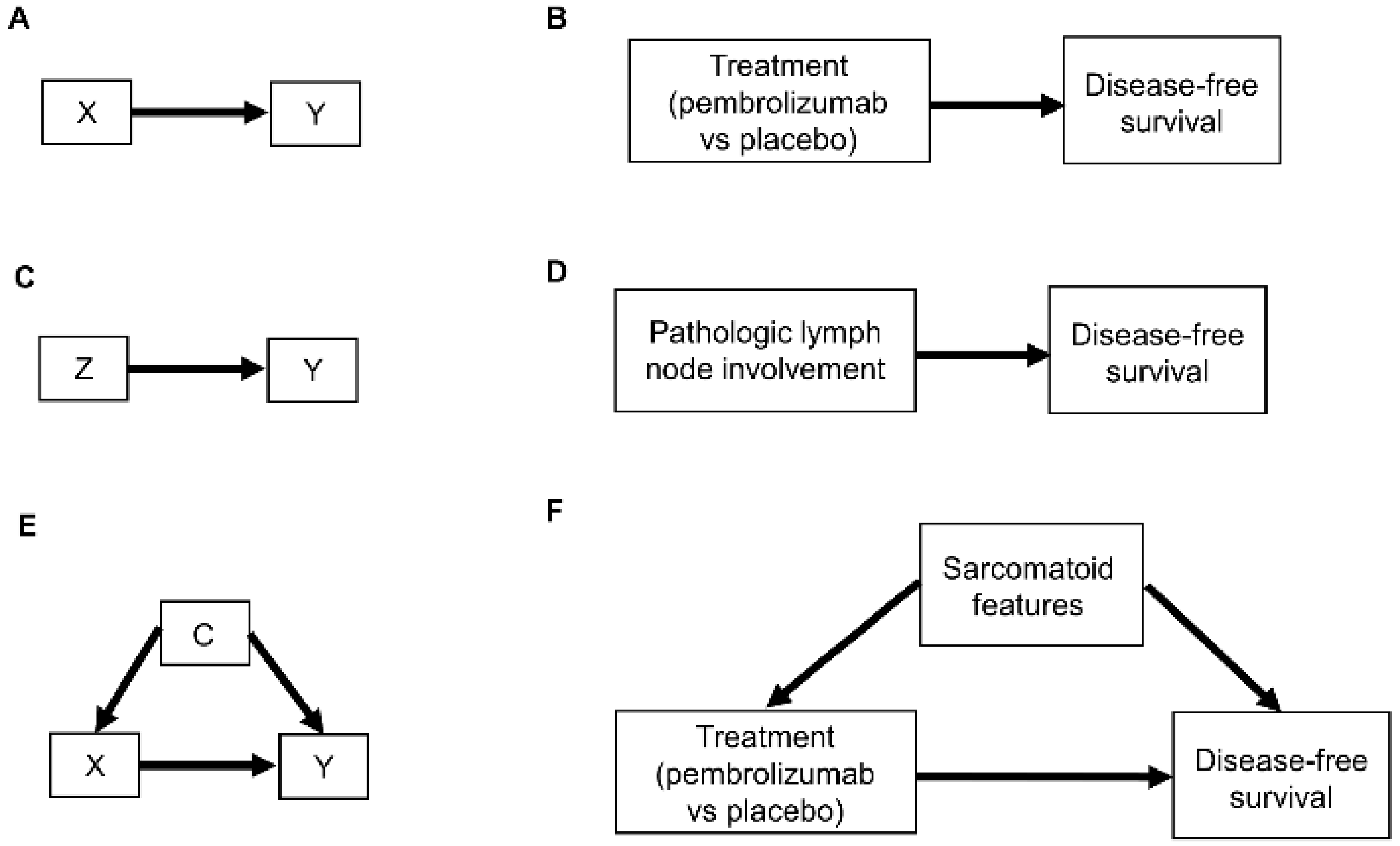
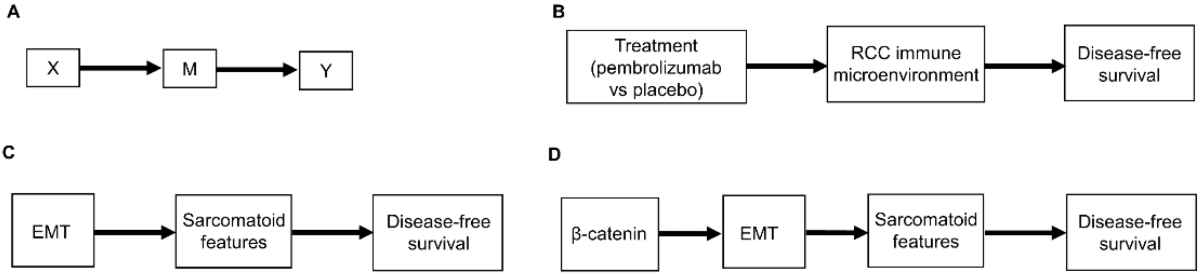
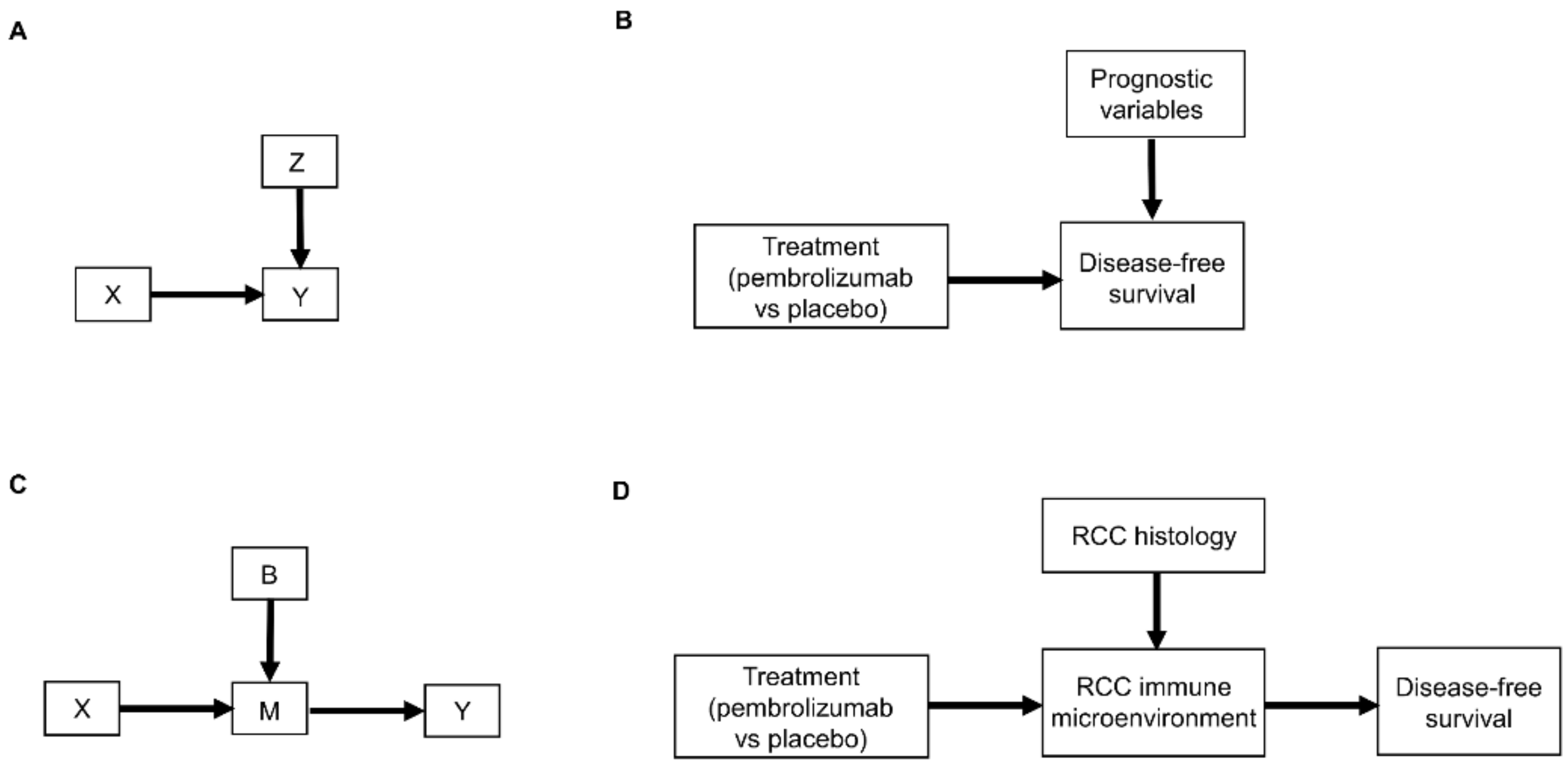
2. Causal Diagrams
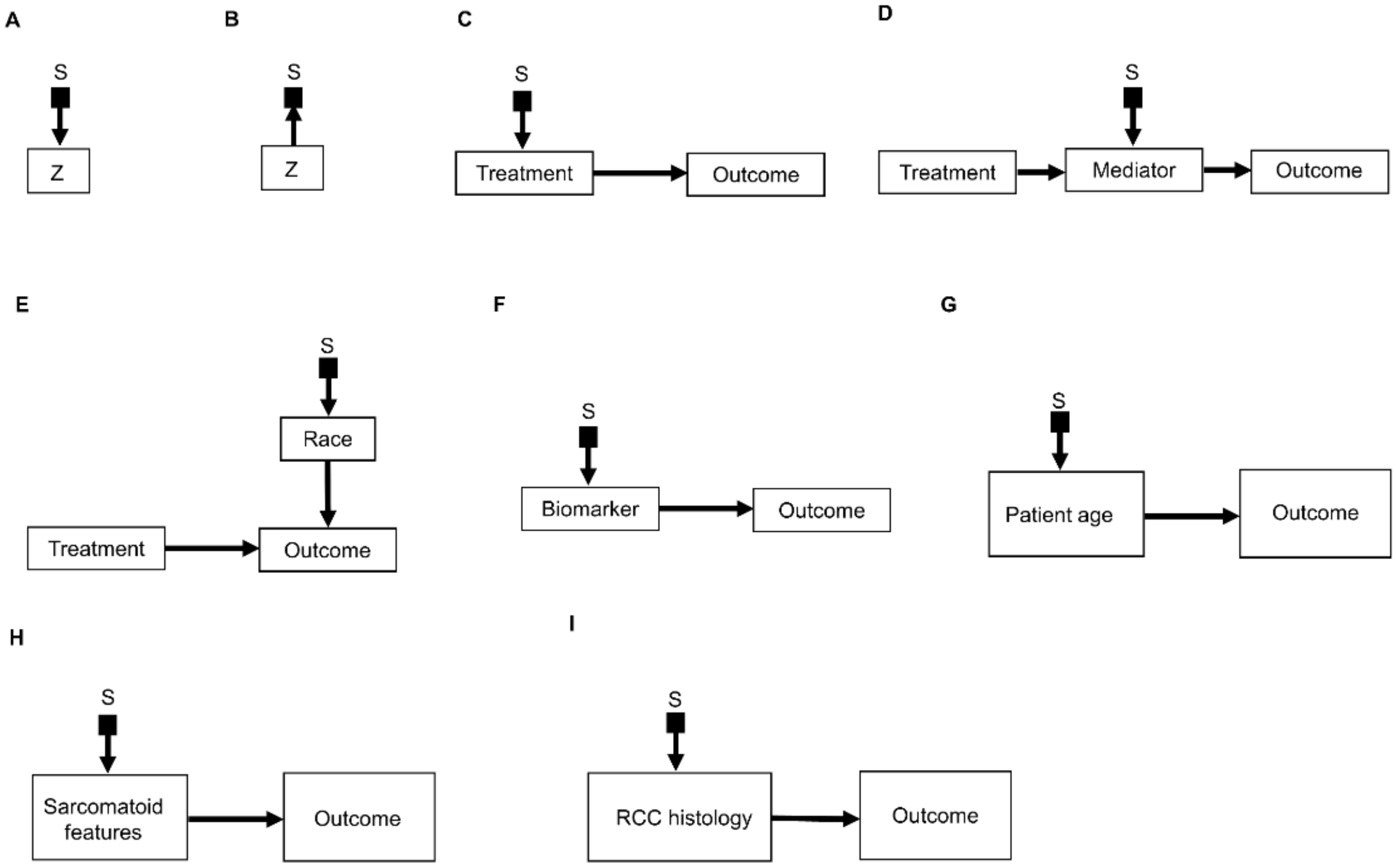
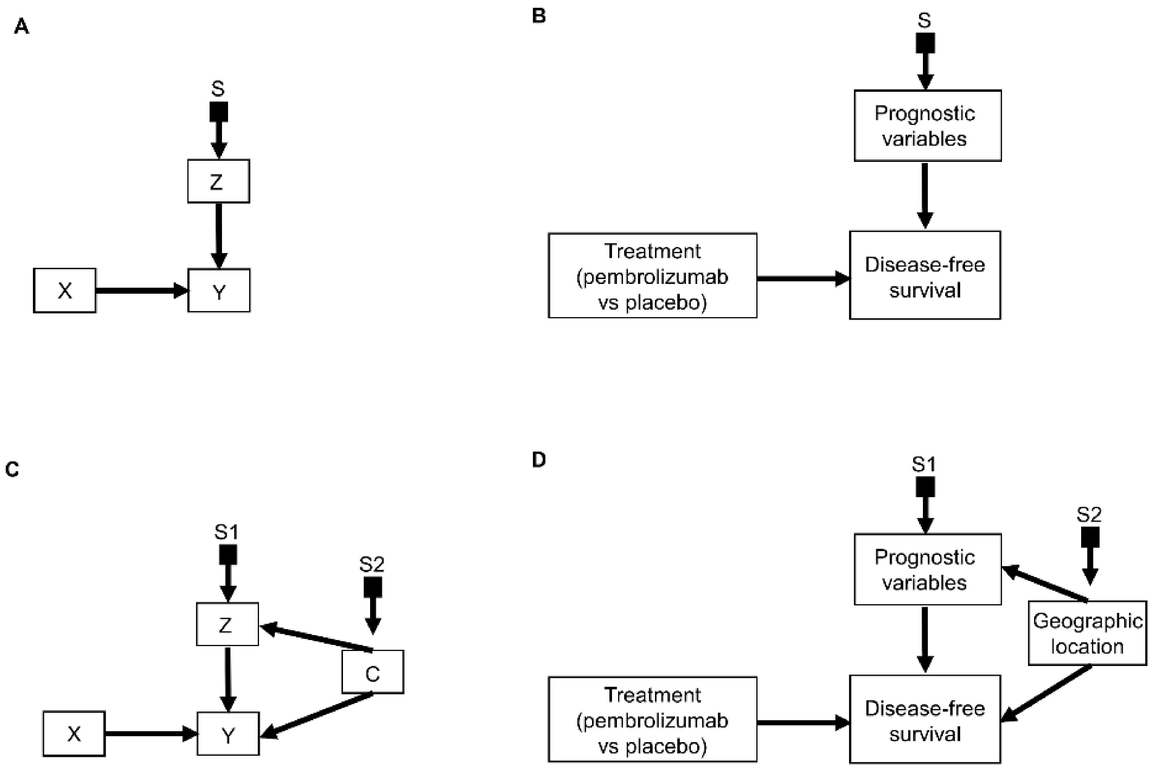
2.1. Selection Diagrams
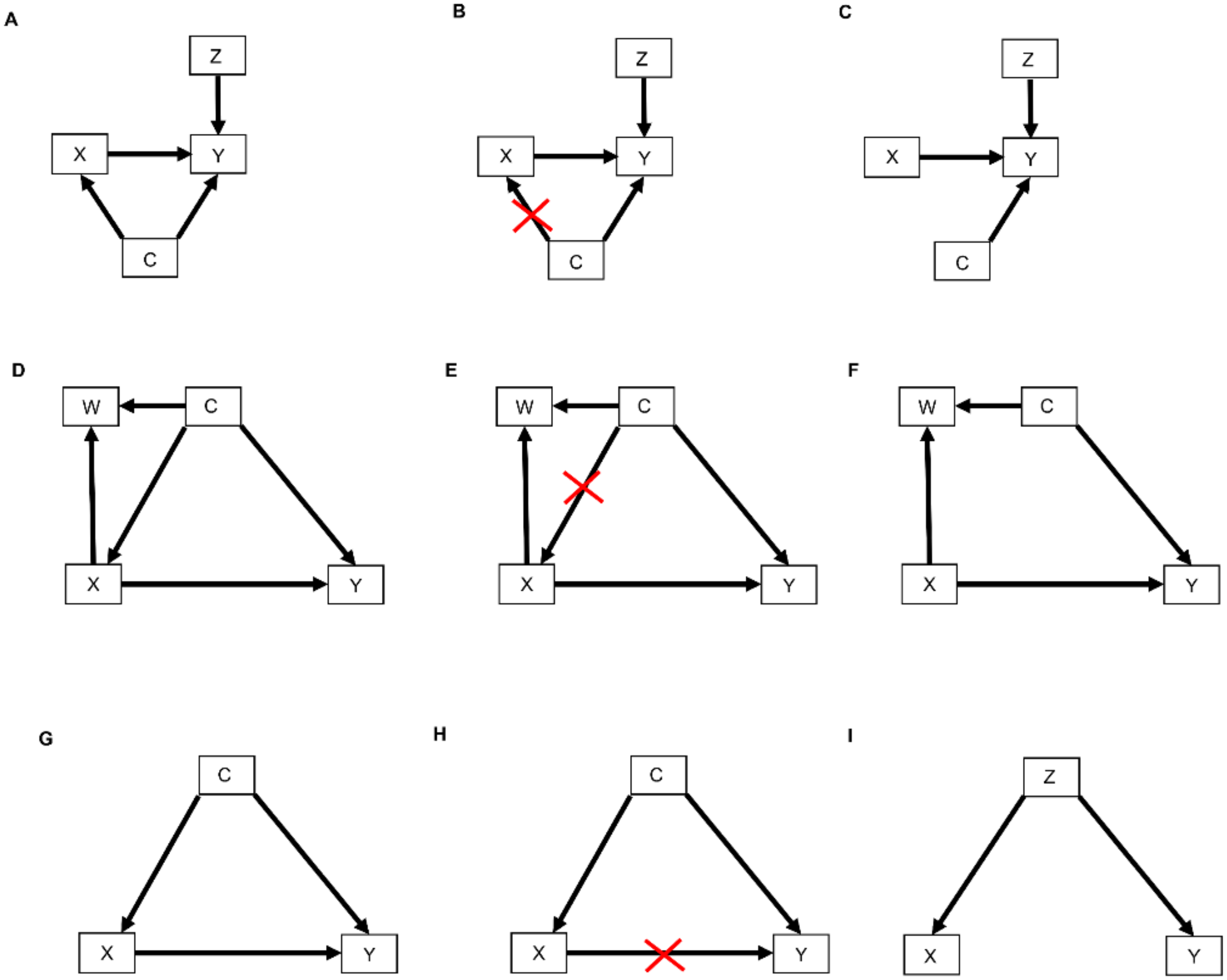
2.2. The Do-Calculus
2.3. Causal Hierarchy
2.4. Causal Inference and Potential Outcomes
3. Causal Modeling of Treatment Effect Heterogeneity
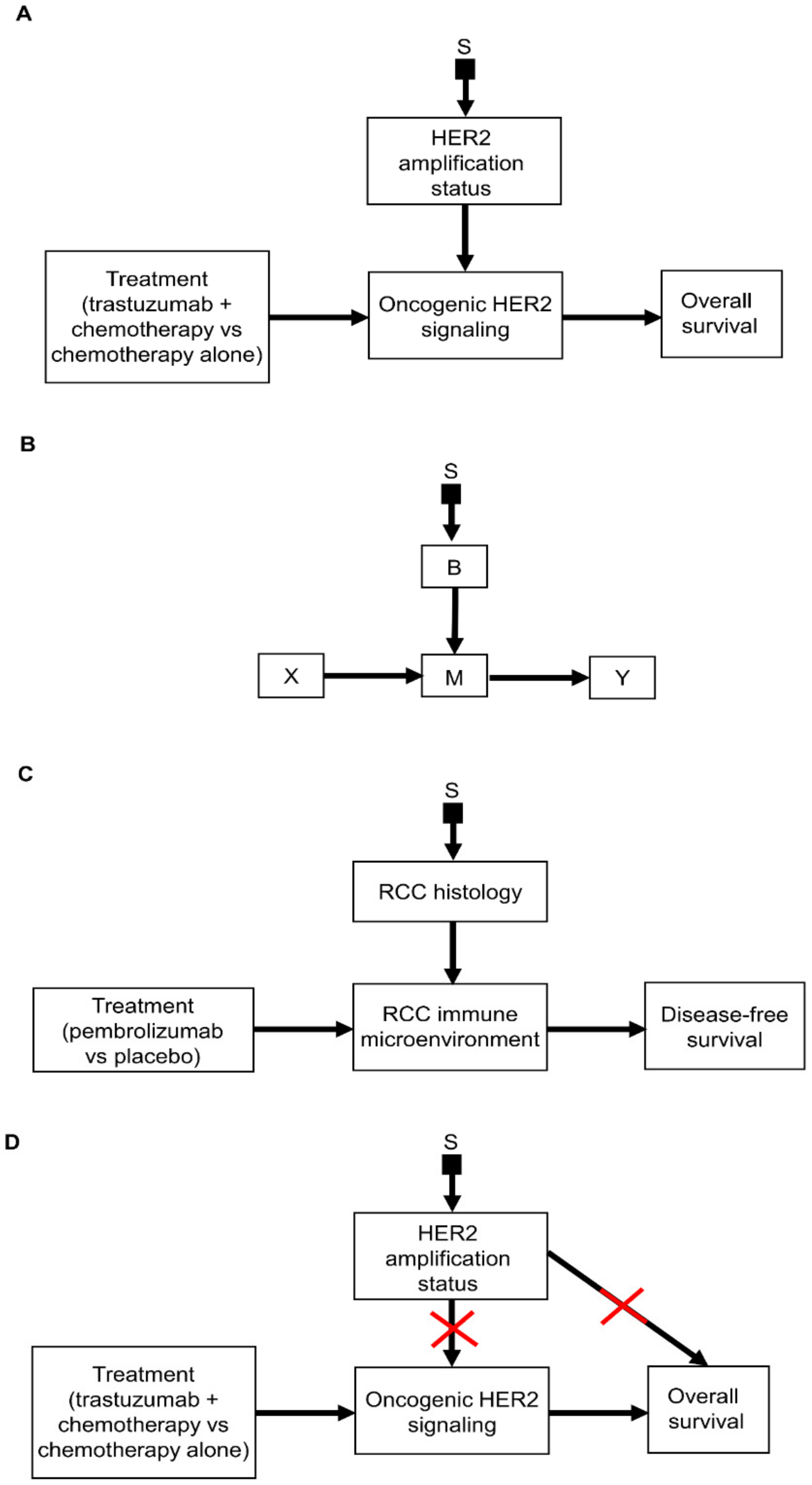
3.1. Causal Diagrams and Interaction Parameters
3.2. Transporting Information across Domains: General Principles
3.3. Transporting Information across Domains: Additive Models
3.4. Transporting Information across Domains: Interactive Models
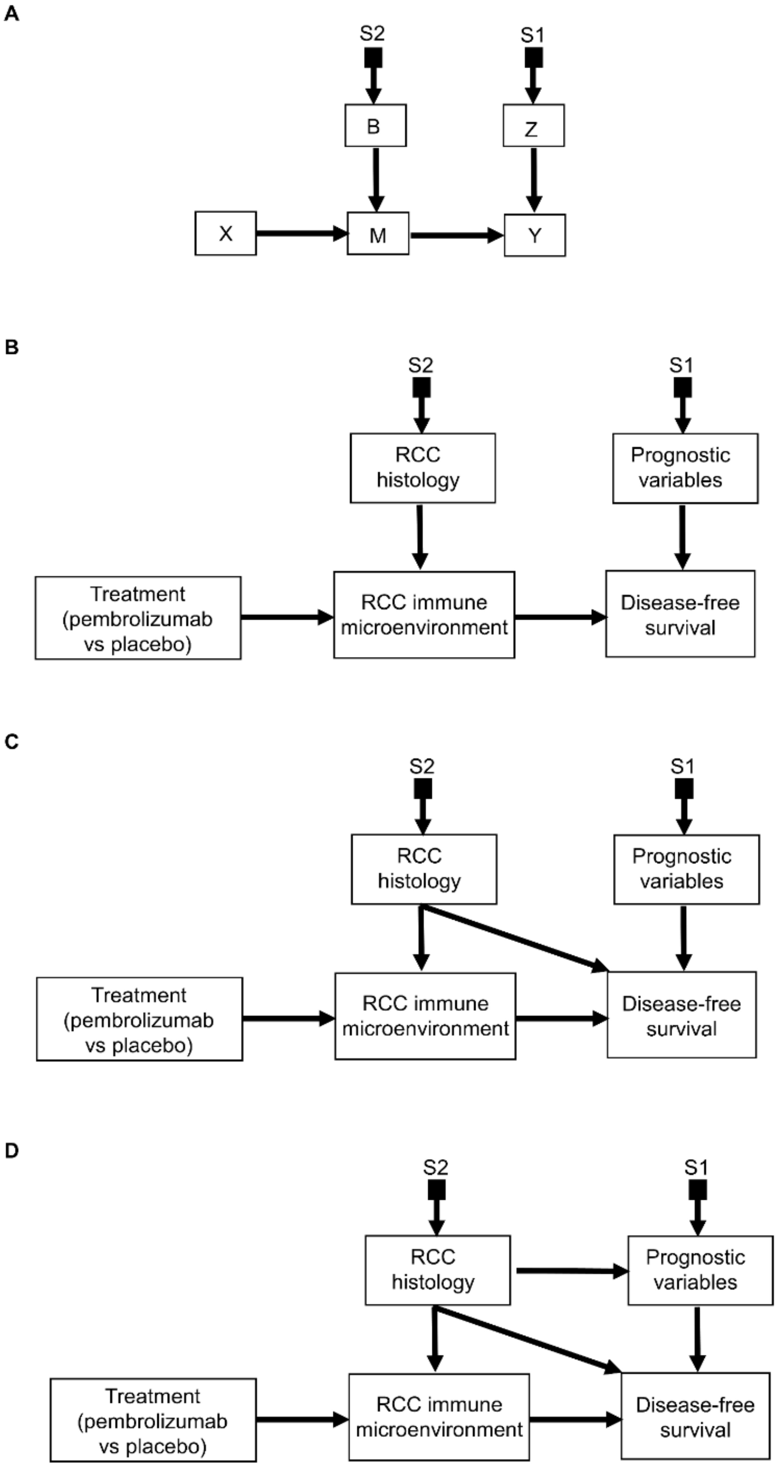
3.5. Transporting Information across Domains: General Framework
3.6. Transporting Information across Domains: More Complex Scenarios
4. Treatment Effect Calculator
5. Clinical Scenarios
5.1. Patient I
5.2. Patient II
5.3. Patient III
5.4. Patient IV
5.5. Patient V
5.6. Patient VI
5.7. Patient VII
5.8. Patient VIII
6. Conclusions
Supplementary Materials
Author Contributions
Funding
Acknowledgments
Conflicts of Interest
References
- Liu, K.; Meng, X.-L. There Is Individualized Treatment. Why Not Individualized Inference? Annu. Rev. Stat. Appl. 2016, 3, 79–111. [Google Scholar] [CrossRef]
- Msaouel, P.; Lee, J.; Thall, P.F. Making Patient-Specific Treatment Decisions Using Prognostic Variables and Utilities of Clinical Outcomes. Cancers 2021, 13, 2741. [Google Scholar] [CrossRef]
- Msaouel, P. Impervious to Randomness: Confounding and Selection Biases in Randomized Clinical Trials. Cancer Investig. 2021, 39, 783–788. [Google Scholar] [CrossRef]
- Shapiro, D.D.; Msaouel, P. Causal Diagram Techniques for Urologic Oncology Research. Clin. Genitourin. Cancer 2021, 19, 271.e1–271.e7. [Google Scholar] [CrossRef] [PubMed]
- Bareinboim, E.; Pearl, J. Causal inference and the data-fusion problem. Proc. Natl. Acad. Sci. USA 2016, 113, 7345–7352. [Google Scholar] [CrossRef]
- Breskin, A.; Cole, S.R.; Edwards, J.K.; Brookmeyer, R.; Eron, J.J.; Adimora, A.A. Fusion designs and estimators for treatment effects. Stat. Med. 2021, 40, 3124–3137. [Google Scholar] [CrossRef] [PubMed]
- Adashek, J.J.; Genovese, G.; Tannir, N.M.; Msaouel, P. Recent advancements in the treatment of metastatic clear cell renal cell carcinoma: A review of the evidence using second-generation p-values. Cancer Treat Res. Commun. 2020, 23, 100166. [Google Scholar] [CrossRef] [PubMed]
- Zoumpourlis, P.; Genovese, G.; Tannir, N.M.; Msaouel, P. Systemic Therapies for the Management of Non-Clear Cell Renal Cell Carcinoma: What Works, What Doesn’t, and What the Future Holds. Clin. Genitourin. Cancer 2021, 19, 103–116. [Google Scholar] [CrossRef] [PubMed]
- Choueiri, T.K.; Tomczak, P.; Park, S.H.; Venugopal, B.; Ferguson, T.; Chang, Y.H.; Hajek, J.; Symeonides, S.N.; Lee, J.L.; Sarwar, N.; et al. Adjuvant Pembrolizumab after Nephrectomy in Renal-Cell Carcinoma. N. Engl. J. Med. 2021, 385, 683–694. [Google Scholar] [CrossRef] [PubMed]
- Msaouel, P.; Grivas, P.; Zhang, T. Adjuvant Systemic Therapies for Patients with Renal Cell Carcinoma: Choosing Treatment Based on Patient-level Characteristics. Eur. Urol. Oncol. 2021, 5, 265–267. [Google Scholar] [CrossRef] [PubMed]
- Correa, A.F.; Jegede, O.A.; Haas, N.B.; Flaherty, K.T.; Pins, M.R.; Adeniran, A.; Messing, E.M.; Manola, J.; Wood, C.G.; Kane, C.J.; et al. Predicting Disease Recurrence, Early Progression, and Overall Survival Following Surgical Resection for High-risk Localized and Locally Advanced Renal Cell Carcinoma. Eur. Urol. 2021, 80, 20–31. [Google Scholar] [CrossRef] [PubMed]
- Ricketts, C.J.; De Cubas, A.A.; Fan, H.; Smith, C.C.; Lang, M.; Reznik, E.; Bowlby, R.; Gibb, E.A.; Akbani, R.; Beroukhim, R.; et al. The Cancer Genome Atlas Comprehensive Molecular Characterization of Renal Cell Carcinoma. Cell Rep. 2018, 23, 313–326.e315. [Google Scholar] [CrossRef]
- Cancer Genome Atlas Research Network. Comprehensive molecular characterization of clear cell renal cell carcinoma. Nature 2013, 499, 43–49. [Google Scholar] [CrossRef] [PubMed]
- Cancer Genome Atlas Research, N.; Linehan, W.M.; Spellman, P.T.; Ricketts, C.J.; Creighton, C.J.; Fei, S.S.; Davis, C.; Wheeler, D.A.; Murray, B.A.; Schmidt, L.; et al. Comprehensive Molecular Characterization of Papillary Renal-Cell Carcinoma. N. Engl. J. Med. 2016, 374, 135–145. [Google Scholar] [CrossRef] [PubMed]
- Davis, C.F.; Ricketts, C.J.; Wang, M.; Yang, L.; Cherniack, A.D.; Shen, H.; Buhay, C.; Kang, H.; Kim, S.C.; Fahey, C.C.; et al. The somatic genomic landscape of chromophobe renal cell carcinoma. Cancer Cell 2014, 26, 319–330. [Google Scholar] [CrossRef] [PubMed]
- Msaouel, P.; Malouf, G.G.; Su, X.; Yao, H.; Tripathi, D.N.; Soeung, M.; Gao, J.; Rao, P.; Coarfa, C.; Creighton, C.J.; et al. Comprehensive Molecular Characterization Identifies Distinct Genomic and Immune Hallmarks of Renal Medullary Carcinoma. Cancer Cell 2020, 37, 720–734.e713. [Google Scholar] [CrossRef] [PubMed]
- Brodaczewska, K.K.; Szczylik, C.; Fiedorowicz, M.; Porta, C.; Czarnecka, A.M. Choosing the right cell line for renal cell cancer research. Mol. Cancer 2016, 15, 83. [Google Scholar] [CrossRef] [PubMed]
- Hsieh, J.J.; Purdue, M.P.; Signoretti, S.; Swanton, C.; Albiges, L.; Schmidinger, M.; Heng, D.Y.; Larkin, J.; Ficarra, V. Renal cell carcinoma. Nat. Rev. Dis. Primers 2017, 3, 17009. [Google Scholar] [CrossRef]
- Wolf, M.M.; Kimryn Rathmell, W.; Beckermann, K.E. Modeling clear cell renal cell carcinoma and therapeutic implications. Oncogene 2020, 39, 3413–3426. [Google Scholar] [CrossRef]
- Piccininni, M.; Konigorski, S.; Rohmann, J.L.; Kurth, T. Directed acyclic graphs and causal thinking in clinical risk prediction modeling. BMC Med. Res. Methodol. 2020, 20, 179. [Google Scholar] [CrossRef]
- Kaplan, E.L.; Meier, P. Nonparametric Estimation from Incomplete Observations. J. Am. Stat. Assoc. 1958, 53, 457–481. [Google Scholar] [CrossRef]
- Hoogland, J.; IntHout, J.; Belias, M.; Rovers, M.M.; Riley, R.D.; Harrell, F.J.E.; Moons, K.G.M.; Debray, T.P.A.; Reitsma, J.B. A tutorial on individualized treatment effect prediction from randomized trials with a binary endpoint. Stat. Med. 2021, 40, 5961–5981. [Google Scholar] [CrossRef] [PubMed]
- Kruskal, W.; Mosteller, F. Representative sampling, IV: The history of the concept in statistics, 1895–1939. Int. Stat. Rev. Rev. Int. De Stat. 1980, 48, 169–195. [Google Scholar] [CrossRef]
- Kruskal, W.; Mosteller, F. Representative sampling, III: The current statistical literature. Int. Stat. Rev. Rev. Int. De Stat. 1979, 47, 245–265. [Google Scholar] [CrossRef]
- Pearl, J. Causality: Models, Reasoning, and Inference, 2nd ed.; Cambridge University Press: Cambridge, UK, 2009; pp. 1–384. [Google Scholar]
- Greenland, S.; Pearl, J.; Robins, J.M. Causal diagrams for epidemiologic research. Epidemiology 1999, 10, 37–48. [Google Scholar] [CrossRef]
- Blum, K.A.; Gupta, S.; Tickoo, S.K.; Chan, T.A.; Russo, P.; Motzer, R.J.; Karam, J.A.; Hakimi, A.A. Sarcomatoid renal cell carcinoma: Biology, natural history and management. Nat. Rev. Urol. 2020, 17, 659–678. [Google Scholar] [CrossRef] [PubMed]
- Kim, J. Events as Property Exemplifications. In Action Theory; Brand, M., Walton, D., Reidel, D., Eds.; Springer: Dordretch, The Netherlands, 1976; pp. 310–326. [Google Scholar]
- Quine, W.V. Events and reification. In Actions and Events: Perspectives on the Philosophy of Davidson; Lepore, E., McLaughlin, B., Eds.; Blackwell: Oxford, UK, 1985; pp. 162–171. [Google Scholar]
- Carmona-Bayonas, A.; Jimenez-Fonseca, P.; Gallego, J.; Msaouel, P. Causal considerations can inform the interpretation of surprising associations in medical registries. Cancer Investig. 2021, 40, 1–27. [Google Scholar] [CrossRef] [PubMed]
- Msaouel, P. The Big Data Paradox in Clinical Practice. Cancer Investig. 2022, 40, 567–576. [Google Scholar] [CrossRef] [PubMed]
- Bareinboim, E.; Pearl, J. Transportability of causal effects: Completeness results. In Proceedings of the Twenty-Sixth AAAI Conference on Artificial Intelligence, Toronto, ON, Canada, 22–26 July; pp. 698–704.
- Correa, J.; Tian, J.; Bareinboim, E. Adjustment Criteria for Generalizing Experimental Findings. In Proceedings of the 36th International Conference on Machine Learning, Proceedings of Machine Learning Research, Long Beach, CA, USA, 9–15 June 2019; pp. 1361–1369. [Google Scholar]
- Pearl, J. Generalizing Experimental Findings. J. Causal Inference 2015, 3, 259–266. [Google Scholar] [CrossRef]
- Bareinboim, E.; Pearl, J. A General Algorithm for Deciding Transportability of Experimental Results. J. Causal Inference 2013, 1, 107–134. [Google Scholar] [CrossRef]
- Pearl, J.; Bareinboim, E. Note on “Generalizability of Study Results”. Epidemiology 2019, 30, 186–188. [Google Scholar] [CrossRef] [PubMed]
- Pearl, J.; Bareinboim, E. External Validity: From Do-Calculus to Transportability Across Populations. Stat. Sci. 2014, 29, 517, 579–595. [Google Scholar] [CrossRef]
- Mishra-Kalyani, P.S.; Amiri Kordestani, L.; Rivera, D.R.; Singh, H.; Ibrahim, A.; DeClaro, R.A.; Shen, Y.; Tang, S.; Sridhara, R.; Kluetz, P.G.; et al. External control arms in oncology: Current use and future directions. Ann. Oncol. 2022, 33, 376–383. [Google Scholar] [CrossRef] [PubMed]
- Hirsch, B.R.; Califf, R.M.; Cheng, S.K.; Tasneem, A.; Horton, J.; Chiswell, K.; Schulman, K.A.; Dilts, D.M.; Abernethy, A.P. Characteristics of oncology clinical trials: Insights from a systematic analysis of ClinicalTrials.gov. JAMA Intern. Med. 2013, 173, 972–979. [Google Scholar] [CrossRef] [PubMed]
- Pearl, J.; Mackenzie, D. The Book of Why: The New Science of Cause and Effect; Basic Books: New York, NY, USA, 2018. [Google Scholar]
- Lewis, D.K. Counterfactuals, Rev. ed.; Blackwell Publishers: Malden, MA, USA, 2001; p. viii. 156p. [Google Scholar]
- VanderWeele, T.J.; Robins, J.M. Directed acyclic graphs, sufficient causes, and the properties of conditioning on a common effect. Am. J. Epidemiol. 2007, 166, 1096–1104. [Google Scholar] [CrossRef]
- Rubin, D.B. Causal Inference Using Potential Outcomes. J. Am. Stat. Assoc. 2005, 100, 322–331. [Google Scholar] [CrossRef]
- Rubin, D.B. Statistics and causal inference: Comment: Which ifs have causal answers. J. Am. Stat. Assoc. 1986, 81, 961–962. [Google Scholar] [CrossRef]
- Oganisian, A.; Roy, J.A. A practical introduction to Bayesian estimation of causal effects: Parametric and nonparametric approaches. Stat. Med. 2021, 40, 518–551. [Google Scholar] [CrossRef]
- Austin, P.C.; Stuart, E.A. Moving towards best practice when using inverse probability of treatment weighting (IPTW) using the propensity score to estimate causal treatment effects in observational studies. Stat. Med. 2015, 34, 3661–3679. [Google Scholar] [CrossRef]
- Rosenbaum, P.R.; Rubin, D.B. The central role of the propensity score in observational studies for causal effects. Biometrika 1983, 70, 41–55. [Google Scholar] [CrossRef]
- Rosenbaum, P.R.; Rubin, D.B. Reducing Bias in Observational Studies Using Subclassification on the Propensity Score. J. Am. Stat. Assoc. 1984, 79, 516–524. [Google Scholar] [CrossRef]
- Bang, H.; Robins, J.M. Doubly robust estimation in missing data and causal inference models. Biometrics 2005, 61, 962–973. [Google Scholar] [CrossRef] [PubMed]
- Naimi, A.I.; Cole, S.R.; Kennedy, E.H. An introduction to g methods. Int. J. Epidemiol. 2017, 46, 756–762. [Google Scholar] [CrossRef] [PubMed]
- Dahabreh, I.J.; Robertson, S.E.; Tchetgen, E.J.; Stuart, E.A.; Hernan, M.A. Generalizing causal inferences from individuals in randomized trials to all trial-eligible individuals. Biometrics 2019, 75, 685–694. [Google Scholar] [CrossRef] [PubMed]
- Lee, D.; Yang, S.; Dong, L.; Wang, X.; Zeng, D.; Cai, J. Improving trial generalizability using observational studies. Biometrics 2022, 1–13. [Google Scholar] [CrossRef]
- Dahabreh, I.J.; Hernan, M.A. Extending inferences from a randomized trial to a target population. Eur. J. Epidemiol. 2019, 34, 719–722. [Google Scholar] [CrossRef]
- Colnet, B.; Mayer, I.; Chen, G.; Dieng, A.; Li, R.; Varoquaux, G.; Vert, J.-P.; Josse, J.; Yang, S. Causal inference methods for combining randomized trials and observational studies: A review. arXiv 2020, arXiv:2011.08047. [Google Scholar]
- Muller, P.; Mitra, R. Bayesian Nonparametric Inference—Why and How. Bayesian Anal. 2013, 8, 269–302. [Google Scholar] [CrossRef]
- Gelman, A.; Hill, J.; Vehtari, A. Regression and Other Stories; Cambridge University Press: Cambridge, UK, 2020. [Google Scholar]
- Harrell, J.F.E. Regression Modeling Strategies: With Applications to Linear Models, Logistic and Ordinal Regression, and Survival Analysis. In Springer Series in Statistics; Springer: Berlin/Heidelberg, Germany, 2015. [Google Scholar] [CrossRef]
- Thall, P.F. Statistical Remedies for Medical Researchers; Springer: Berlin/Heidelberg, Germany, 2020. [Google Scholar]
- Rindskopf, D. Reporting Bayesian Results. Eval. Rev. 2020, 44, 354–375. [Google Scholar] [CrossRef]
- Krnjajić, M.; Draper, D. Bayesian model comparison: Log scores and DIC. Stat. Amp. Probab. Lett. 2014, 88, 9–14. [Google Scholar] [CrossRef]
- Heinze, G.; Wallisch, C.; Dunkler, D. Variable selection—A review and recommendations for the practicing statistician. Biom. J. 2018, 60, 431–449. [Google Scholar] [CrossRef] [PubMed]
- Schad, D.J.; Betancourt, M.; Vasishth, S. Toward a principled Bayesian workflow in cognitive science. Psychol. Methods 2021, 26, 103–126. [Google Scholar] [CrossRef] [PubMed]
- Rahman, R.; Fell, G.; Ventz, S.; Arfe, A.; Vanderbeek, A.M.; Trippa, L.; Alexander, B.M. Deviation from the Proportional Hazards Assumption in Randomized Phase 3 Clinical Trials in Oncology: Prevalence, Associated Factors, and Implications. Clin. Cancer Res. 2019, 25, 6339–6345. [Google Scholar] [CrossRef] [PubMed]
- Thall, P.F.; Mueller, P.; Xu, Y.; Guindani, M. Bayesian nonparametric statistics: A new toolkit for discovery in cancer research. Pharm. Stat. 2017, 16, 414–423. [Google Scholar] [CrossRef] [PubMed]
- MacEachern, S.N. Nonparametric Bayesian methods: A gentle introduction and overview. Commun. Stat. Appl. Methods 2016, 23, 445–466. [Google Scholar] [CrossRef]
- Xu, Y.; Muller, P.; Wahed, A.S.; Thall, P.F. Bayesian Nonparametric Estimation for Dynamic Treatment Regimes with Sequential Transition Times. J. Am. Stat. Assoc. 2016, 111, 921–935. [Google Scholar] [CrossRef]
- Kent, D.M.; Paulus, J.K.; van Klaveren, D.; D’Agostino, R.; Goodman, S.; Hayward, R.; Ioannidis, J.P.A.; Patrick-Lake, B.; Morton, S.; Pencina, M.; et al. The Predictive Approaches to Treatment effect Heterogeneity (PATH) Statement. Ann. Intern. Med. 2020, 172, 35–45. [Google Scholar] [CrossRef]
- Kent, D.M.; van Klaveren, D.; Paulus, J.K.; D’Agostino, R.; Goodman, S.; Hayward, R.; Ioannidis, J.P.A.; Patrick-Lake, B.; Morton, S.; Pencina, M.; et al. The Predictive Approaches to Treatment effect Heterogeneity (PATH) Statement: Explanation and Elaboration. Ann. Intern. Med. 2020, 172, W1–W25. [Google Scholar] [CrossRef]
- Cuzick, J. Prognosis vs Treatment Interaction. JNCI Cancer Spectr. 2018, 2, pky006. [Google Scholar] [CrossRef]
- Ballman, K.V. Biomarker: Predictive or Prognostic? J. Clin. Oncol. 2015, 33, 3968–3971. [Google Scholar] [CrossRef]
- Huitfeldt, A.; Swanson, S.A.; Stensrud, M.J.; Suzuki, E. Effect heterogeneity and variable selection for standardizing causal effects to a target population. Eur. J. Epidemiol. 2019, 34, 1119–1129. [Google Scholar] [CrossRef] [PubMed]
- Snapinn, S.; Jiang, Q. On the clinical meaningfulness of a treatment’s effect on a time-to-event variable. Stat. Med. 2011, 30, 2341–2348. [Google Scholar] [CrossRef] [PubMed]
- Vander Weele, T.J. Confounding and effect modification: Distribution and measure. Epidemiol. Methods 2012, 1, 55–82. [Google Scholar] [CrossRef]
- Msaouel, P.; Jimenez-Fonseca, P.; Lim, B.; Carmona-Bayonas, A.; Agnelli, G. Medicine before and after David Cox. Eur. J. Intern. Med. 2022, 98, 1–3. [Google Scholar] [CrossRef] [PubMed]
- Thall, P.F. Bayesian cancer clinical trial designs with subgroup-specific decisions. Contemp. Clin. Trials 2020, 90, 105860. [Google Scholar] [CrossRef] [PubMed]
- Park, Y.; Liu, S.; Thall, P.F.; Yuan, Y. Bayesian group sequential enrichment designs based on adaptive regression of response and survival time on baseline biomarkers. Biometrics 2021, 78, 60–71. [Google Scholar] [CrossRef]
- Murray, T.A.; Yuan, Y.; Thall, P.F. A Bayesian Machine Learning Approach for Optimizing Dynamic Treatment Regimes. J. Am. Stat. Assoc. 2018, 113, 1255–1267. [Google Scholar] [CrossRef]
- Chipman, H.A.; George, E.I.; McCulloch, R.E. BART: Bayesian additive regression trees. Ann. Appl. Stat. 2010, 4, 266–298, 233. [Google Scholar] [CrossRef]
- Lee, H.K.H. Bayesian Nonparametrics via Neural Networks; SIAM ASA, American Statistical Association: Philadelphia, PA, USA; Alexandria, VA, USA, 2004; p. 96. [Google Scholar]
- Ligon, B.L. Penicillin: Its discovery and early development. Semin. Pediatr. Infect. Dis. 2004, 15, 52–57. [Google Scholar] [CrossRef]
- Goldstein, I.; Burnett, A.L.; Rosen, R.C.; Park, P.W.; Stecher, V.J. The Serendipitous Story of Sildenafil: An Unexpected Oral Therapy for Erectile Dysfunction. Sex Med. Rev. 2019, 7, 115–128. [Google Scholar] [CrossRef]
- Singh, R.K.; Kumar, S.; Prasad, D.N.; Bhardwaj, T.R. Therapeutic journery of nitrogen mustard as alkylating anticancer agents: Historic to future perspectives. Eur. J. Med. Chem. 2018, 151, 401–433. [Google Scholar] [CrossRef] [PubMed]
- Modi, S.; Jacot, W.; Yamashita, T.; Sohn, J.; Vidal, M.; Tokunaga, E.; Tsurutani, J.; Ueno, N.T.; Prat, A.; Chae, Y.S.; et al. Trastuzumab Deruxtecan in Previously Treated HER2-Low Advanced Breast Cancer. N. Engl. J. Med. 2022, 387, 9–20. [Google Scholar] [CrossRef] [PubMed]
- Pearl, J.; Bareinboim, E. Transportability of Causal and Statistical Relations: A Formal Approach. In Proceedings of the 2011 IEEE 11th International Conference on Data Mining Workshops, Vancouver, BC, Canada, 11 December 2011; pp. 540–547. [Google Scholar]
- Haas, N.B.; Manola, J.; Uzzo, R.G.; Flaherty, K.T.; Wood, C.G.; Kane, C.; Jewett, M.; Dutcher, J.P.; Atkins, M.B.; Pins, M.; et al. Adjuvant sunitinib or sorafenib for high-risk, non-metastatic renal-cell carcinoma (ECOG-ACRIN E2805): A double-blind, placebo-controlled, randomised, phase 3 trial. Lancet 2016, 387, 2008–2016. [Google Scholar] [CrossRef]
- Fletcher, R.H.; Fletcher, S.W.; Fletcher, G.S. Clinical Epidemiology: The Essentials, 5th ed.; Wolters Kluwer/Lippincott Williams & Wilkins Health: Philadelphia, PA, USA, 2014; p. 253. [Google Scholar]
- Rothman, K.J.; Gallacher, J.E.; Hatch, E.E. Why representativeness should be avoided. Int. J. Epidemiol. 2013, 42, 1012–1014. [Google Scholar] [CrossRef] [PubMed]
- Elwood, J.M. Commentary: On representativeness. Int. J. Epidemiol. 2013, 42, 1014–1015. [Google Scholar] [CrossRef]
- Richiardi, L.; Pizzi, C.; Pearce, N. Commentary: Representativeness is usually not necessary and often should be avoided. Int. J. Epidemiol. 2013, 42, 1018–1022. [Google Scholar] [CrossRef]
- Capitanio, U.; Bensalah, K.; Bex, A.; Boorjian, S.A.; Bray, F.; Coleman, J.; Gore, J.L.; Sun, M.; Wood, C.; Russo, P. Epidemiology of Renal Cell Carcinoma. Eur. Urol. 2019, 75, 74–84. [Google Scholar] [CrossRef]
- Sperrin, M.; Jenkins, D.; Martin, G.P.; Peek, N. Explicit causal reasoning is needed to prevent prognostic models being victims of their own success. J. Am. Med. Inf. Assoc. 2019, 26, 1675–1676. [Google Scholar] [CrossRef]
- Greenland, S.; Pearce, N. Statistical foundations for model-based adjustments. Annu. Rev. Public Health 2015, 36, 89–108. [Google Scholar] [CrossRef]
- Lipkovich, I.; Dmitrienko, A.; D’ Agostino, S.B.R. Tutorial in biostatistics: Data-driven subgroup identification and analysis in clinical trials. Stat. Med. 2017, 36, 136–196. [Google Scholar] [CrossRef]
- Thall, P.F.; Wathen, J.K.; Bekele, B.N.; Champlin, R.E.; Baker, L.H.; Benjamin, R.S. Hierarchical Bayesian approaches to phase II trials in diseases with multiple subtypes. Stat. Med. 2003, 22, 763–780. [Google Scholar] [CrossRef] [PubMed]
- Graziani, R.; Guindani, M.; Thall, P.F. Bayesian nonparametric estimation of targeted agent effects on biomarker change to predict clinical outcome. Biometrics 2015, 71, 188–197. [Google Scholar] [CrossRef] [PubMed]
- Renfro, L.A.; Mallick, H.; An, M.W.; Sargent, D.J.; Mandrekar, S.J. Clinical trial designs incorporating predictive biomarkers. Cancer Treat. Rev. 2016, 43, 74–82. [Google Scholar] [CrossRef] [PubMed]
- Kent, D.M.; Steyerberg, E.; van Klaveren, D. Personalized evidence based medicine: Predictive approaches to heterogeneous treatment effects. BMJ 2018, 363, k4245. [Google Scholar] [CrossRef]
- Chia, P.L.; Gedye, C.; Boutros, P.C.; Wheatley-Price, P.; John, T. Current and Evolving Methods to Visualize Biological Data in Cancer Research. J. Natl. Cancer Inst. 2016, 108, djw031. [Google Scholar] [CrossRef]
- Hahn, A.W.; Dizman, N.; Msaouel, P. Missing the trees for the forest: Most subgroup analyses using forest plots at the ASCO annual meeting are inconclusive. Adv. Med. Oncol. 2022, 14, 17588359221103199. [Google Scholar] [CrossRef]
- Senn, S. Statistical Issues in Drug Development, 3rd ed.; John Wiley and Sons, Ltd.: Hoboken, NJ, USA, 2021. [Google Scholar]
- Spears, M.R.; James, N.D.; Sydes, M.R. ‘Thursday’s child has far to go’—interpreting subgroups and the STAMPEDE trial. Ann. Oncol. 2017, 28, 2327–2330. [Google Scholar] [CrossRef]
- Sun, X.; Briel, M.; Walter, S.D.; Guyatt, G.H. Is a subgroup effect believable? Updating criteria to evaluate the credibility of subgroup analyses. BMJ 2010, 340, c117. [Google Scholar] [CrossRef]
- Sun, X.; Ioannidis, J.P.; Agoritsas, T.; Alba, A.C.; Guyatt, G. How to use a subgroup analysis: Users’ guide to the medical literature. JAMA 2014, 311, 405–411. [Google Scholar] [CrossRef]
- Hayes, D.F. HER2 and Breast Cancer—A Phenomenal Success Story. N. Engl. J. Med. 2019, 381, 1284–1286. [Google Scholar] [CrossRef]
- Falzone, L.; Salomone, S.; Libra, M. Evolution of Cancer Pharmacological Treatments at the Turn of the Third Millennium. Front. Pharm. 2018, 9, 1300. [Google Scholar] [CrossRef] [PubMed]
- Slamon, D.J.; Clark, G.M.; Wong, S.G.; Levin, W.J.; Ullrich, A.; McGuire, W.L. Human breast cancer: Correlation of relapse and survival with amplification of the HER-2/neu oncogene. Science 1987, 235, 177–182. [Google Scholar] [CrossRef]
- Slamon, D.J.; Godolphin, W.; Jones, L.A.; Holt, J.A.; Wong, S.G.; Keith, D.E.; Levin, W.J.; Stuart, S.G.; Udove, J.; Ullrich, A.; et al. Studies of the HER-2/neu proto-oncogene in human breast and ovarian cancer. Science 1989, 244, 707–712. [Google Scholar] [CrossRef] [PubMed]
- Zabrecky, J.R.; Lam, T.; McKenzie, S.J.; Carney, W. The extracellular domain of p185/neu is released from the surface of human breast carcinoma cells, SK-BR-3. J. Biol. Chem. 1991, 266, 1716–1720. [Google Scholar] [CrossRef]
- Scott, G.K.; Robles, R.; Park, J.W.; Montgomery, P.A.; Daniel, J.; Holmes, W.E.; Lee, J.; Keller, G.A.; Li, W.L.; Fendly, B.M.; et al. A truncated intracellular HER2/neu receptor produced by alternative RNA processing affects growth of human carcinoma cells. Mol. Cell Biol. 1993, 13, 2247–2257. [Google Scholar] [CrossRef] [PubMed]
- Liu, Y.; el-Ashry, D.; Chen, D.; Ding, I.Y.; Kern, F.G. MCF-7 breast cancer cells overexpressing transfected c-erbB-2 have an in vitro growth advantage in estrogen-depleted conditions and reduced estrogen-dependence and tamoxifen-sensitivity in vivo. Breast Cancer Res. Treat 1995, 34, 97–117. [Google Scholar] [CrossRef] [PubMed]
- Eisenhauer, E.A. From the molecule to the clinic—Inhibiting HER2 to treat breast cancer. N. Engl. J. Med. 2001, 344, 841–842. [Google Scholar] [CrossRef]
- Carter, P.; Presta, L.; Gorman, C.M.; Ridgway, J.B.; Henner, D.; Wong, W.L.; Rowland, A.M.; Kotts, C.; Carver, M.E.; Shepard, H.M. Humanization of an anti-p185HER2 antibody for human cancer therapy. Proc. Natl. Acad. Sci. USA 1992, 89, 4285–4289. [Google Scholar] [CrossRef] [PubMed]
- Slamon, D.J.; Leyland-Jones, B.; Shak, S.; Fuchs, H.; Paton, V.; Bajamonde, A.; Fleming, T.; Eiermann, W.; Wolter, J.; Pegram, M.; et al. Use of chemotherapy plus a monoclonal antibody against HER2 for metastatic breast cancer that overexpresses HER2. N. Engl. J. Med. 2001, 344, 783–792. [Google Scholar] [CrossRef] [PubMed]
- Cooke, T.; Reeves, J.; Lanigan, A.; Stanton, P. HER2 as a prognostic and predictive marker for breast cancer. Ann. Oncol. 2001, 12 (Suppl 1), S23–S28. [Google Scholar] [CrossRef] [PubMed]
- Meier, P.; Karrison, T.; Chappell, R.; Xie, H. The Price of Kaplan–Meier. J. Am. Stat. Assoc. 2004, 99, 890–896. [Google Scholar] [CrossRef]
- Miller, R.G., Jr. What price Kaplan-Meier? Biometrics 1983, 39, 1077–1081. [Google Scholar] [CrossRef] [PubMed]
- Han, G.; Schell, M.J.; Zhang, H.; Zelterman, D.; Pusztai, L.; Adelson, K.; Hatzis, C. Testing violations of the exponential assumption in cancer clinical trials with survival endpoints. Biometrics 2017, 73, 687–695. [Google Scholar] [CrossRef]
- Xu, Y.; Thall, P.F.; Hua, W.; Andersson, B.S. Bayesian non-parametric survival regression for optimizing precision dosing of intravenous busulfan in allogeneic stem cell transplantation. J. R. Stat. Society. Ser. C Appl. Stat. 2019, 68, 809–828. [Google Scholar] [CrossRef] [PubMed]
- Lee, J.; Thall, P.F.; Msaouel, P. Precision Bayesian phase I–II dose-finding based on utilities tailored to prognostic subgroups. Stat. Med. 2021, 40, 5199–5217. [Google Scholar] [CrossRef] [PubMed]
- Bajorin, D.F.; Witjes, J.A.; Gschwend, J.E.; Schenker, M.; Valderrama, B.P.; Tomita, Y.; Bamias, A.; Lebret, T.; Shariat, S.F.; Park, S.H.; et al. Adjuvant Nivolumab versus Placebo in Muscle-Invasive Urothelial Carcinoma. N. Engl. J. Med. 2021, 384, 2102–2114. [Google Scholar] [CrossRef]
- Birtle, A.; Johnson, M.; Chester, J.; Jones, R.; Dolling, D.; Bryan, R.T.; Harris, C.; Winterbottom, A.; Blacker, A.; Catto, J.W.F.; et al. Adjuvant chemotherapy in upper tract urothelial carcinoma (the POUT trial): A phase 3, open-label, randomised controlled trial. Lancet 2020, 395, 1268–1277. [Google Scholar] [CrossRef]
- Wu, Y.L.; Tsuboi, M.; He, J.; John, T.; Grohe, C.; Majem, M.; Goldman, J.W.; Laktionov, K.; Kim, S.W.; Kato, T.; et al. Osimertinib in Resected EGFR-Mutated Non-Small-Cell Lung Cancer. N. Engl. J. Med. 2020, 383, 1711–1723. [Google Scholar] [CrossRef] [PubMed]
- Tutt, A.N.J.; Garber, J.E.; Kaufman, B.; Viale, G.; Fumagalli, D.; Rastogi, P.; Gelber, R.D.; de Azambuja, E.; Fielding, A.; Balmana, J.; et al. Adjuvant Olaparib for Patients with BRCA1- or BRCA2-Mutated Breast Cancer. N. Engl. J. Med. 2021, 384, 2394–2405. [Google Scholar] [CrossRef]
- Bergerot, C.D.; Battle, D.; Philip, E.J.; Bergerot, P.G.; Msaouel, P.; Smith, A.; Bamgboje, A.E.; Shuch, B.; Derweesh, I.H.; Jonasch, E.; et al. Fear of Cancer Recurrence in Patients with Localized Renal Cell Carcinoma. JCO Oncol. Pract. 2020, 16, e1264–e1271. [Google Scholar] [CrossRef] [PubMed]
- Wang, L.; Rotnitzky, A.; Lin, X.; Millikan, R.E.; Thall, P.F. Evaluation of Viable Dynamic Treatment Regimes in a Sequentially Randomized Trial of Advanced Prostate Cancer. J. Am. Stat. Assoc. 2012, 107, 493–508. [Google Scholar] [CrossRef] [PubMed]
- Kattan, M.W.; Reuter, V.; Motzer, R.J.; Katz, J.; Russo, P. A postoperative prognostic nomogram for renal cell carcinoma. J. Urol. 2001, 166, 63–67. [Google Scholar] [CrossRef]
- Sorbellini, M.; Kattan, M.W.; Snyder, M.E.; Reuter, V.; Motzer, R.; Goetzl, M.; McKiernan, J.; Russo, P. A postoperative prognostic nomogram predicting recurrence for patients with conventional clear cell renal cell carcinoma. J. Urol. 2005, 173, 48–51. [Google Scholar] [CrossRef] [PubMed]
- Zisman, A.; Pantuck, A.J.; Wieder, J.; Chao, D.H.; Dorey, F.; Said, J.W.; deKernion, J.B.; Figlin, R.A.; Belldegrun, A.S. Risk group assessment and clinical outcome algorithm to predict the natural history of patients with surgically resected renal cell carcinoma. J. Clin. Oncol. 2002, 20, 4559–4566. [Google Scholar] [CrossRef] [PubMed]
- Leibovich, B.C.; Blute, M.L.; Cheville, J.C.; Lohse, C.M.; Frank, I.; Kwon, E.D.; Weaver, A.L.; Parker, A.S.; Zincke, H. Prediction of progression after radical nephrectomy for patients with clear cell renal cell carcinoma: A stratification tool for prospective clinical trials. Cancer 2003, 97, 1663–1671. [Google Scholar] [CrossRef] [PubMed]
- Frank, I.; Blute, M.L.; Cheville, J.C.; Lohse, C.M.; Weaver, A.L.; Zincke, H. An outcome prediction model for patients with clear cell renal cell carcinoma treated with radical nephrectomy based on tumor stage, size, grade and necrosis: The SSIGN score. J. Urol. 2002, 168, 2395–2400. [Google Scholar] [CrossRef]
- Thompson, R.H.; Leibovich, B.C.; Lohse, C.M.; Cheville, J.C.; Zincke, H.; Blute, M.L.; Frank, I. Dynamic outcome prediction in patients with clear cell renal cell carcinoma treated with radical nephrectomy: The D-SSIGN score. J. Urol. 2007, 177, 477–480. [Google Scholar] [CrossRef] [PubMed]
- Cindolo, L.; de la Taille, A.; Messina, G.; Romis, L.; Abbou, C.C.; Altieri, V.; Rodriguez, A.; Patard, J.J. A preoperative clinical prognostic model for non-metastatic renal cell carcinoma. BJU Int. 2003, 92, 901–905. [Google Scholar] [CrossRef]
- Karakiewicz, P.I.; Suardi, N.; Capitanio, U.; Jeldres, C.; Ficarra, V.; Cindolo, L.; de la Taille, A.; Tostain, J.; Mulders, P.F.; Bensalah, K.; et al. A preoperative prognostic model for patients treated with nephrectomy for renal cell carcinoma. Eur. Urol. 2009, 55, 287–295. [Google Scholar] [CrossRef] [PubMed]
- Yaycioglu, O.; Roberts, W.W.; Chan, T.; Epstein, J.I.; Marshall, F.F.; Kavoussi, L.R. Prognostic assessment of nonmetastatic renal cell carcinoma: A clinically based model. Urology 2001, 58, 141–145. [Google Scholar] [CrossRef]
- Powles, T.; Assaf, Z.J.; Davarpanah, N.; Banchereau, R.; Szabados, B.E.; Yuen, K.C.; Grivas, P.; Hussain, M.; Oudard, S.; Gschwend, J.E.; et al. ctDNA guiding adjuvant immunotherapy in urothelial carcinoma. Nature 2021, 595, 432–437. [Google Scholar] [CrossRef]
- Nuzzo, P.V.; Berchuck, J.E.; Korthauer, K.; Spisak, S.; Nassar, A.H.; Abou Alaiwi, S.; Chakravarthy, A.; Shen, S.Y.; Bakouny, Z.; Boccardo, F.; et al. Detection of renal cell carcinoma using plasma and urine cell-free DNA methylomes. Nat. Med. 2020, 26, 1041–1043. [Google Scholar] [CrossRef] [PubMed]
- Brookman-May, S.D.; May, M.; Shariat, S.F.; Novara, G.; Zigeuner, R.; Cindolo, L.; De Cobelli, O.; De Nunzio, C.; Pahernik, S.; Wirth, M.P.; et al. Time to recurrence is a significant predictor of cancer-specific survival after recurrence in patients with recurrent renal cell carcinoma—Results from a comprehensive multi-centre database (CORONA/SATURN-Project). BJU Int. 2013, 112, 909–916. [Google Scholar] [CrossRef] [PubMed]
- Kroeger, N.; Choueiri, T.K.; Lee, J.L.; Bjarnason, G.A.; Knox, J.J.; MacKenzie, M.J.; Wood, L.; Srinivas, S.; Vaishamayan, U.N.; Rha, S.Y.; et al. Survival outcome and treatment response of patients with late relapse from renal cell carcinoma in the era of targeted therapy. Eur. Urol. 2014, 65, 1086–1092. [Google Scholar] [CrossRef]
- Tang, C.; Msaouel, P.; Hara, K.; Choi, H.; Le, V.; Shah, A.Y.; Wang, J.; Jonasch, E.; Choi, S.; Nguyen, Q.N.; et al. Definitive radiotherapy in lieu of systemic therapy for oligometastatic renal cell carcinoma: A single-arm, single-centre, feasibility, phase 2 trial. Lancet Oncol. 2021, 22, P1732–P1739. [Google Scholar] [CrossRef]
- Linehan, W.M.; Ricketts, C.J. The Cancer Genome Atlas of renal cell carcinoma: Findings and clinical implications. Nat. Rev. Urol. 2019, 16, 539–552. [Google Scholar] [CrossRef]
- Montironi, R.; Cimadamore, A.; Ohashi, R.; Cheng, L.; Scarpelli, M.; Lopez-Beltran, A.; Moch, H. Chromophobe Renal Cell Carcinoma Aggressiveness and Immuno-oncology Therapy: How to Distinguish the Good One from the Bad One. Eur. Urol. Oncol. 2021, 4, 331–333. [Google Scholar] [CrossRef]
- Ohashi, R.; Martignoni, G.; Hartmann, A.; Calio, A.; Segala, D.; Stohr, C.; Wach, S.; Erlmeier, F.; Weichert, W.; Autenrieth, M.; et al. Multi-institutional re-evaluation of prognostic factors in chromophobe renal cell carcinoma: Proposal of a novel two-tiered grading scheme. Virchows Arch. 2020, 476, 409–418. [Google Scholar] [CrossRef]
- Neves, J.B.; Vanaclocha Saiz, L.; Abu-Ghanem, Y.; Marchetti, M.; Tran-Dang, M.A.; El-Sheikh, S.; Barod, R.; Beisland, C.; Capitanio, U.; Cullen, D.; et al. Pattern, timing and predictors of recurrence after surgical resection of chromophobe renal cell carcinoma. World J. Urol. 2021, 39, 3823–3831. [Google Scholar] [CrossRef]

| Intermediate-High Risk | High Risk | M1 with No Evidence of Disease | |||
|---|---|---|---|---|---|
| Pathologic primary tumor (T) stage | pT2 | pT3 | pT4 | Any pT | Any pT |
| Tumor nuclear grade | Grade 4 or sarcomatoid | Any grade | Any grade | Any grade | Any grade |
| Regional lymph node (N) stage | N0 | N0 | N0 | N1 | Any lymph node stage |
| Metastatic stage | M0 | M0 | M0 | M0 | M1 |
| pT2: primary tumor >7 cm in greatest dimension, limited to the kidney pT3: primary tumor extends into major veins or perinephric tissues, but not into the ipsilateral adrenal gland and not beyond Gerota’s fascia pT4: Tumor invades beyond Gerota’s fascia (including contiguous extension into the ipsilateral adrenal gland) N0: No regional lymph node metastasis N1: Metastasis in regional lymph node(s) M0: No history of radiologically visible distant metastasis M1: History of radiologically visible distant metastasis | |||||
| Layer | Activity | Analysis Unit | Mathematical Expression | Example Query |
|---|---|---|---|---|
| One | Observation | Population | P(Y | Z) | What is the DFS time distribution in patients at high risk for ccRCC recurrence? |
| Two | Intervention | Population | P(Y | do(X = 1)) | What is the DFS time distribution in patients with ccRCC treated with adjuvant pembrolizumab? |
| Three | Potential outcomes | Individual Patient | E(YX = 1 | Z = 1) − E(YX = 0 | Z = 1) | What would the expected DFS time be if I treat a patient with high-risk ccRCC with adjuvant pembrolizumab compared to placebo? |
| Type of Adjuvant Therapy | Milestone Time (Months) | Reported Milestone DFS Probability in Control Group | Estimated HR and CIs for DFS | Estimated Milestone DFS Probability in Treatment Group | Reported Milestone DFS Probability in Treatment Group | Difference between Estimated Versus Reported Milestone DFS Probability | Reference |
|---|---|---|---|---|---|---|---|
| Immune checkpoint therapy vs. placebo | 12 | 76.2% | 0.68 | 83.1% | 85.7% | −2.6% | [9] |
| Immune checkpoint therapy vs. placebo | 24 | 68.1% | 0.68 | 77% | 77.3% | −0.3% | [9] |
| Immune checkpoint therapy vs. placebo | 6 | 60.3% | 0.70 | 70.2% | 74.9% | −4.7% | [120] |
| Chemotherapy vs. placebo | 36 | 46% | 0.45 | 70.5% | 71% | −0.5% | [121] |
| Targeted therapy vs. placebo | 24 | 52% | 0.20 | 87.7% | 89% | −1.3% | [122] |
| Targeted therapy vs. placebo | 36 | 80.4% | 0.57 | 88.3% | 87.5% | +0.8% | [123] |
| Patient | RCC Histology | Eligible for KN-564 | Age | Tumor Stage | Tumor Size (cm) | Fuhrman Nuclear grade | Necrosis | Renal Vein Invasion | Sarcomatoid features | Predicted 2-Year DFS with Surveillance | Predicted 2-Year DFS with Pembrolizumab | ARR | Recommend Adjuvant Pembrolizumab | External Observational Studies Needed | External Experimental Studies Needed |
|---|---|---|---|---|---|---|---|---|---|---|---|---|---|---|---|
| I | Clear cell | Yes | 48 | pT3a pN0 M0 | 10.6 | 4 | Yes | Yes | Yes | 41.1% | 54.9% | 13.5% | Yes | No | No |
| II | Clear cell | Yes | 48 | pT3a pN0 M0 | 7.0 | 2 | No | Yes | No | 87.2% | 91.1% | 3.9% | No | No | No |
| III | Clear cell | No | 55 | pT2b pN0 M0 | 10.3 | 3 | Yes | No | No | 68% | 76.9% | 8.9% | Yes | No | No |
| IV | Clear cell | Yes | 52 | pT3a pN0 M1 NED | 10.2 | 3 | No | Yes | No | Not estimable | Not estimable | Not estimable | Not estimable | Yes | No |
| V | Papillary type I | No | 54 | pT3a pN0 M0 | 13.9 | 2 | No | Yes | No | 94.6% | Not formally estimable but would be 97.3% even if HR = 0.5 | Not formally estimable but would be 2.7% even if HR = 0.5 | No | No | Yes |
| VI | Papillary type II | No | 49 | pT3 pN0 M0 | 10.4 | 4 | Yes | Yes | Yes | 41.4% | Not formally estimable but would be 47.7% even if hazard ratio (HR) = 0.84 | Not formally estimable but would be 6.3% even if HR = 0.84 | Not formally estimable but is a plausible recommendation under current state of knowledge | No | Yes |
| VII | Chromo-phobe | No | 56 | pT2a pN0 M0 | 9.5 | Low grade | No | No | No | 97.9% | Not formally estimable but would be 98.9% even if HR = 0.5 | Not formally estimable but would be 1% even if HR = 0.5 | No | No | Yes |
| VIII | Chromo-phobe | No | 52 | pT2b pN0 M0 | 11.4 | High grade | No | No | Yes | Not estimable | Not estimable | Not estimable | Not estimable | Yes | Yes |
| pT2a: primary tumor >7 cm but ≤10cm in greatest dimension, limited to the kidney pT2b: primary tumor >10 cm in greatest dimension, limited to the kidney pT3a: primary tumor extends into the renal vein or its segmental (muscle containing) branches, or tumor invades perirenal and/or renal sinus fat (ie, perinephric fat), but not into the ipsilateral adrenal gland and not beyond Gerota’s fascia pN0: No regional lymph node metastasis M0: No history of radiologically visible distant metastasis M1 NED: History of radiologically visible distant metastasis with currently no evidence of disease | |||||||||||||||
Publisher’s Note: MDPI stays neutral with regard to jurisdictional claims in published maps and institutional affiliations. |
© 2022 by the authors. Licensee MDPI, Basel, Switzerland. This article is an open access article distributed under the terms and conditions of the Creative Commons Attribution (CC BY) license (https://creativecommons.org/licenses/by/4.0/).
Share and Cite
Msaouel, P.; Lee, J.; Karam, J.A.; Thall, P.F. A Causal Framework for Making Individualized Treatment Decisions in Oncology. Cancers 2022, 14, 3923. https://doi.org/10.3390/cancers14163923
Msaouel P, Lee J, Karam JA, Thall PF. A Causal Framework for Making Individualized Treatment Decisions in Oncology. Cancers. 2022; 14(16):3923. https://doi.org/10.3390/cancers14163923
Chicago/Turabian StyleMsaouel, Pavlos, Juhee Lee, Jose A. Karam, and Peter F. Thall. 2022. "A Causal Framework for Making Individualized Treatment Decisions in Oncology" Cancers 14, no. 16: 3923. https://doi.org/10.3390/cancers14163923
APA StyleMsaouel, P., Lee, J., Karam, J. A., & Thall, P. F. (2022). A Causal Framework for Making Individualized Treatment Decisions in Oncology. Cancers, 14(16), 3923. https://doi.org/10.3390/cancers14163923