
An Enhanced Histopathology Analysis: An AI-Based System for Multiclass Grading of Oral Squamous Cell Carcinoma and Segmenting of Epithelial and Stromal Tissue

 , , , , and
Simple Summary
Abstract
1. Introduction
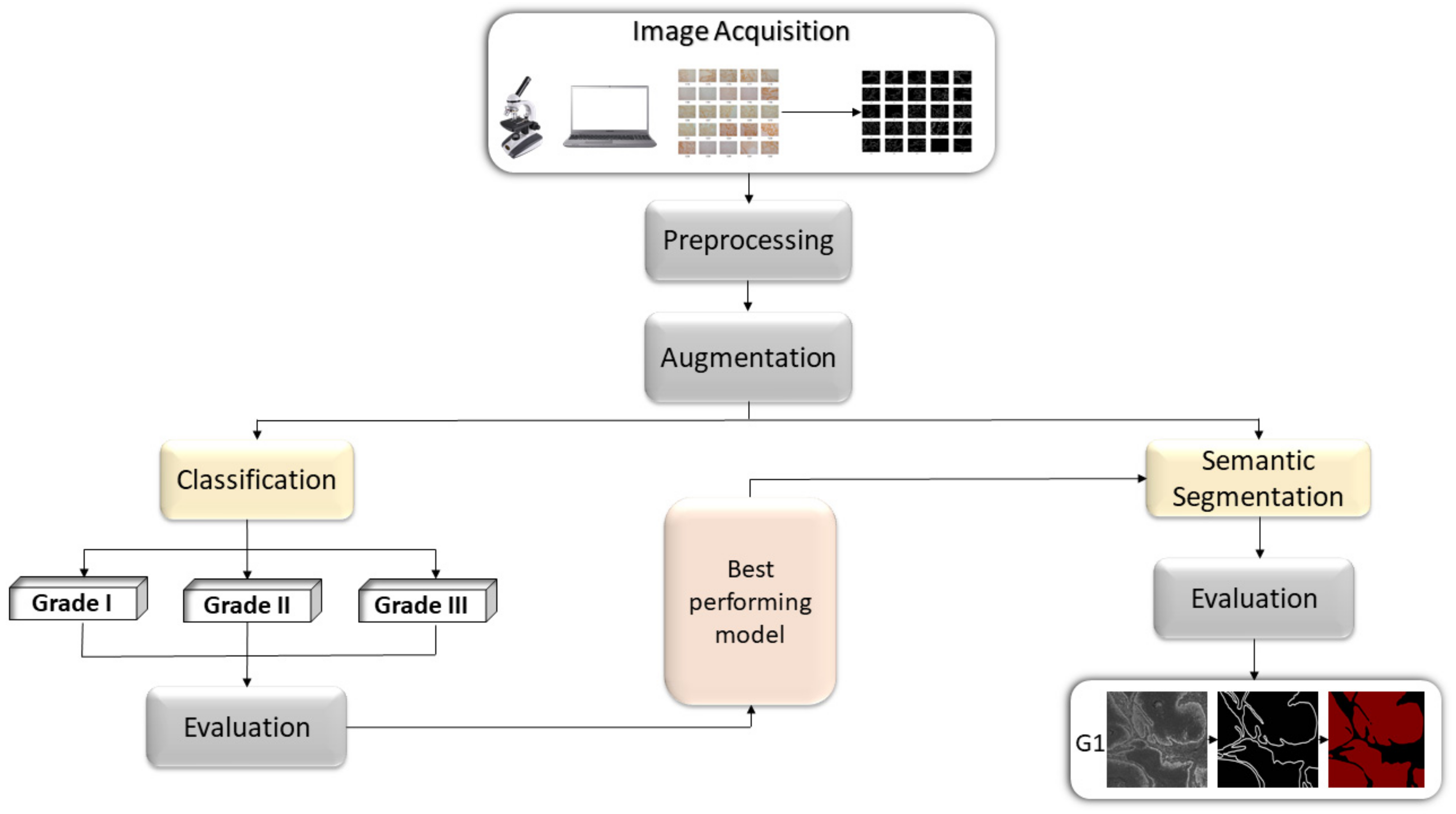
- The first stage of an AI-based system for multiclass grading of OSCC which can potentially improve objectivity and reproducibility of histopathological examination, as well as reduce the time necessary for pathological inspections.
- The second stage of an AI-based system for segmentation of tumor on epithelial and stromal regions which can assist the clinician in discovering new informative features. It has great potential in the quantification of qualitative clinic-pathological features in order to predict tumor invasion and metastasis.
- A new preprocessing methodology based on the stationary wavelet transform (SWT) is proposed to enhance high-frequency components in the case of multiclass classification and to extract low-level features in the case of semantic segmentation. This approach allows more effective predictions and improves the robustness of the entire AI-based system.
Related Work
2. Materials and Methods
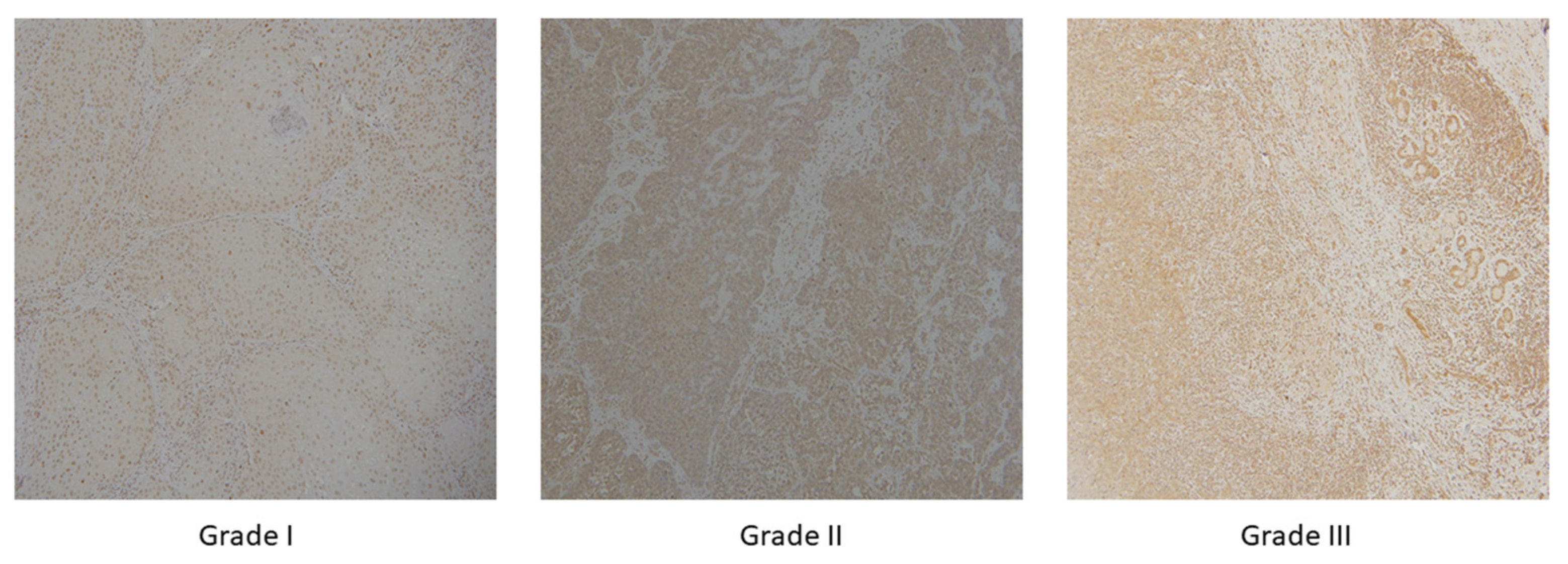
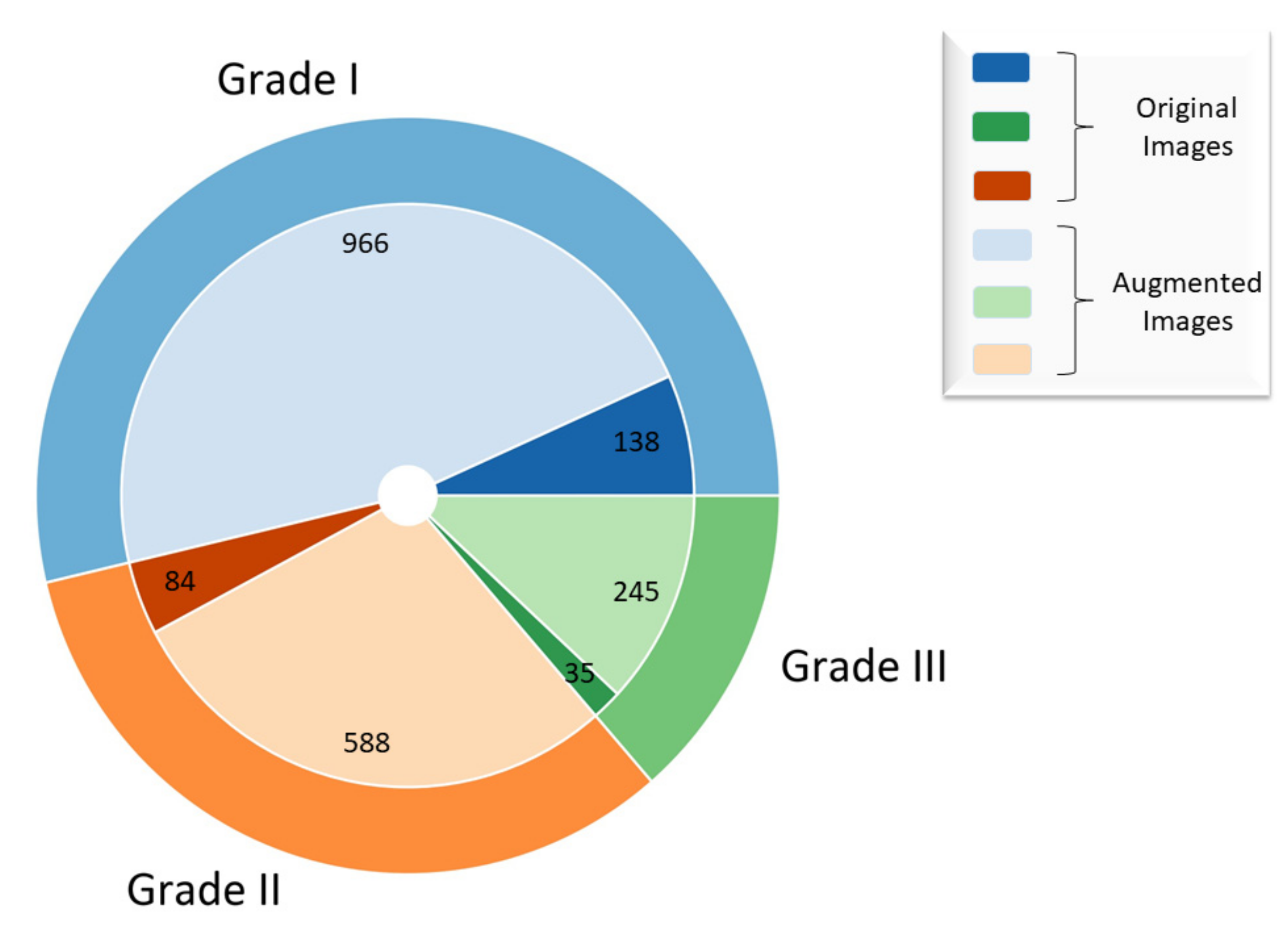
2.1. Dataset Description
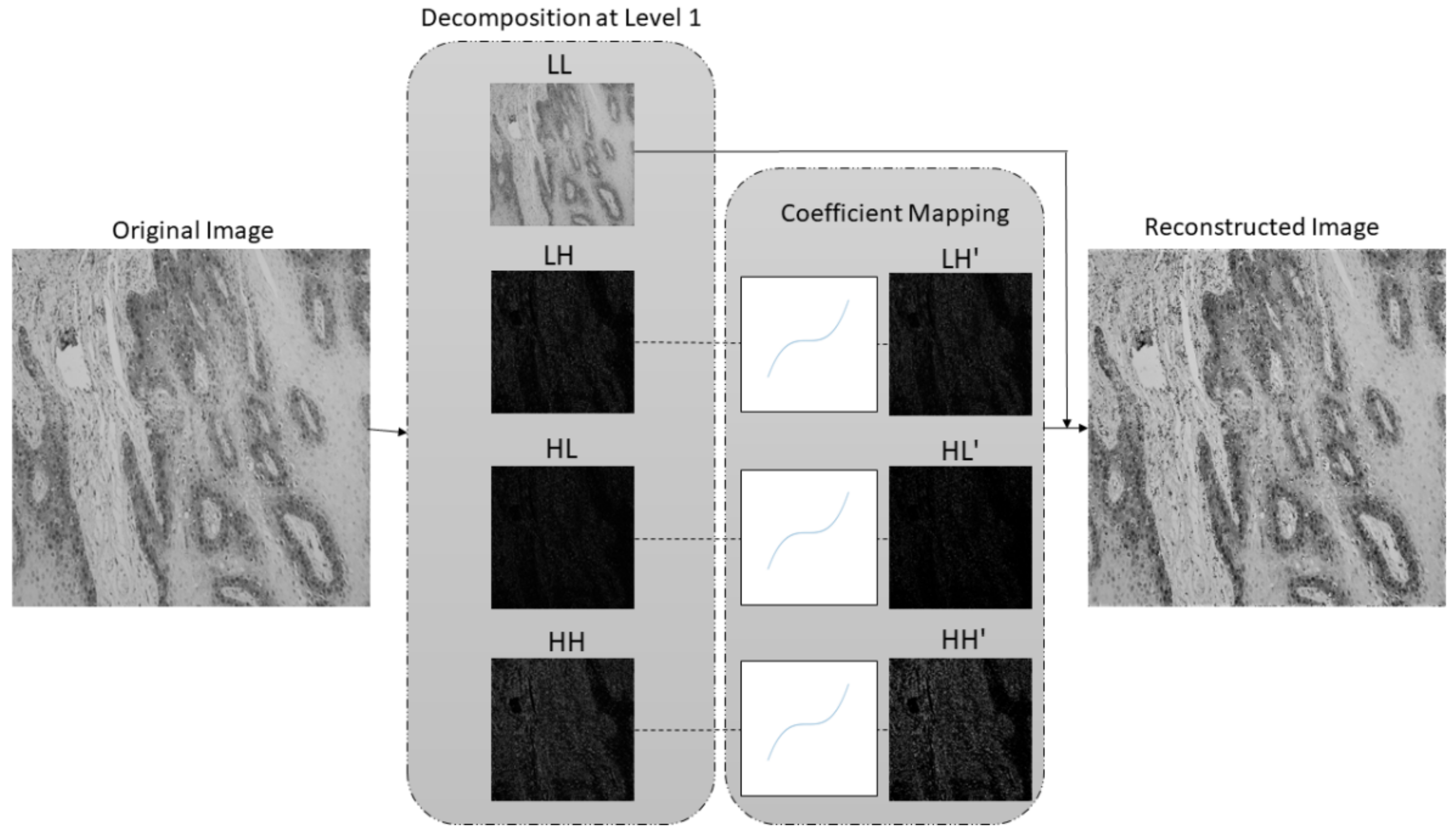
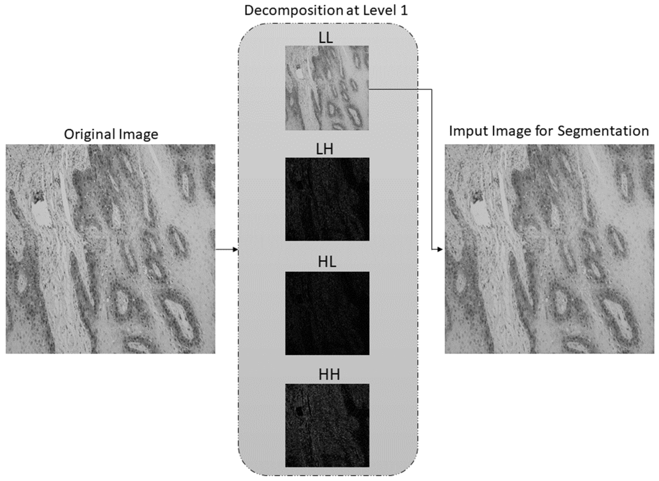
2.2. Preprocessing Method Based on Stationary Wavelet Transform and Mapping Function
- no decimation step—provides redundant information,
- better time-frequency localization, and
- translation-invariance.
2.3. AI-Based Models
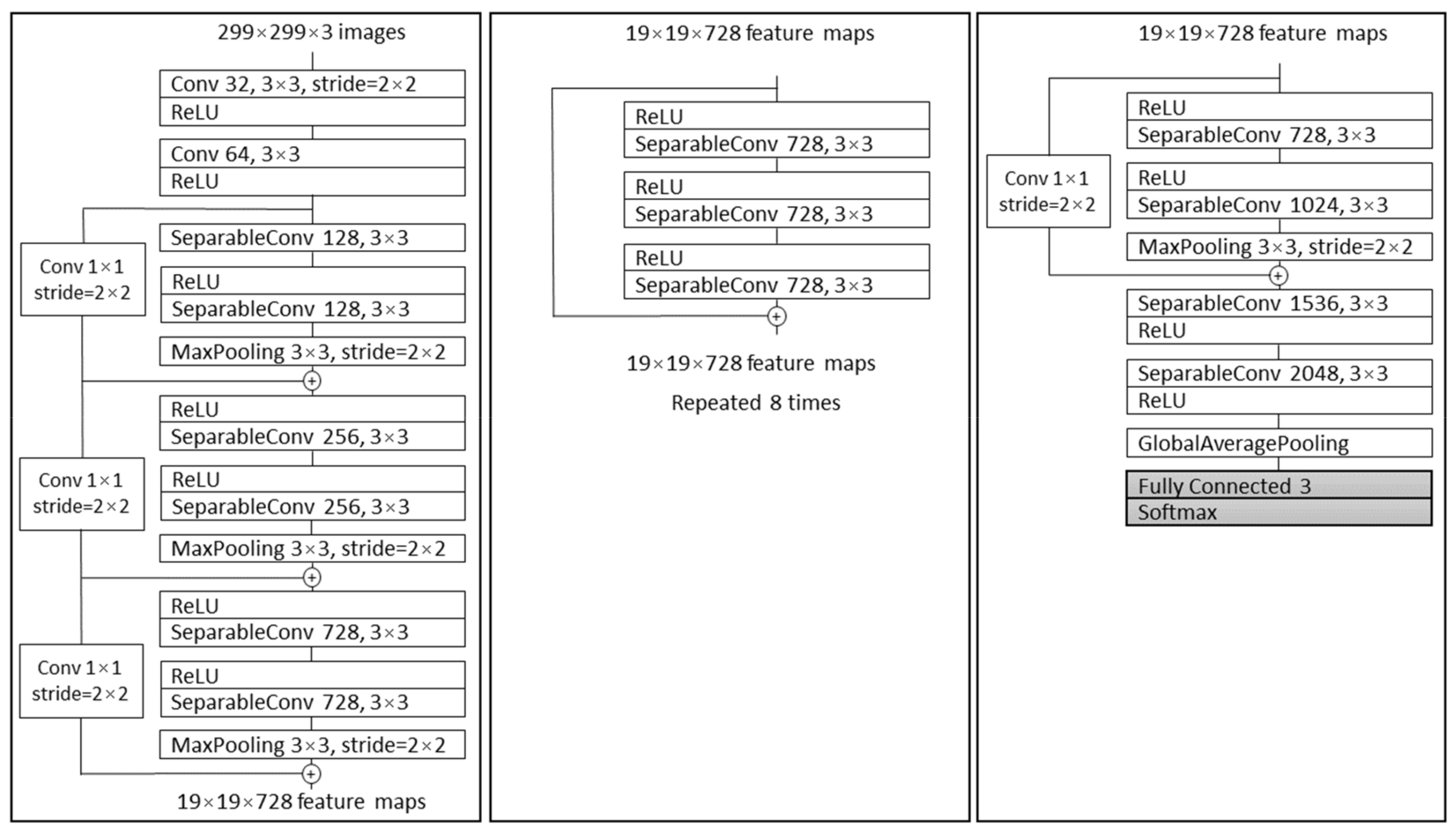
2.3.1. Xception
2.3.2. ResNet50 and −101
2.3.3. MobileNetv2
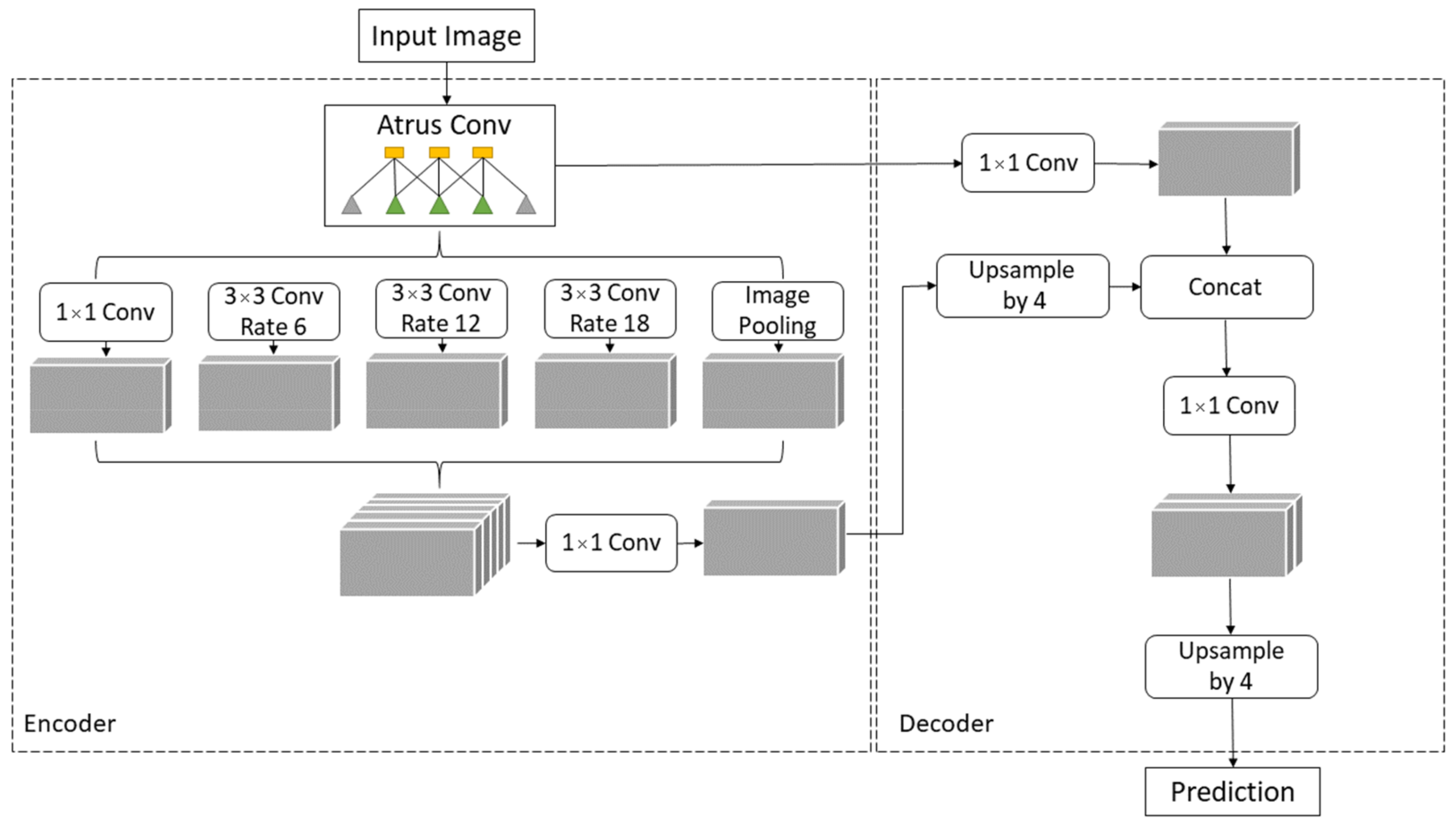
2.4. DeepLabv3+
2.5. Evaluation Criteria
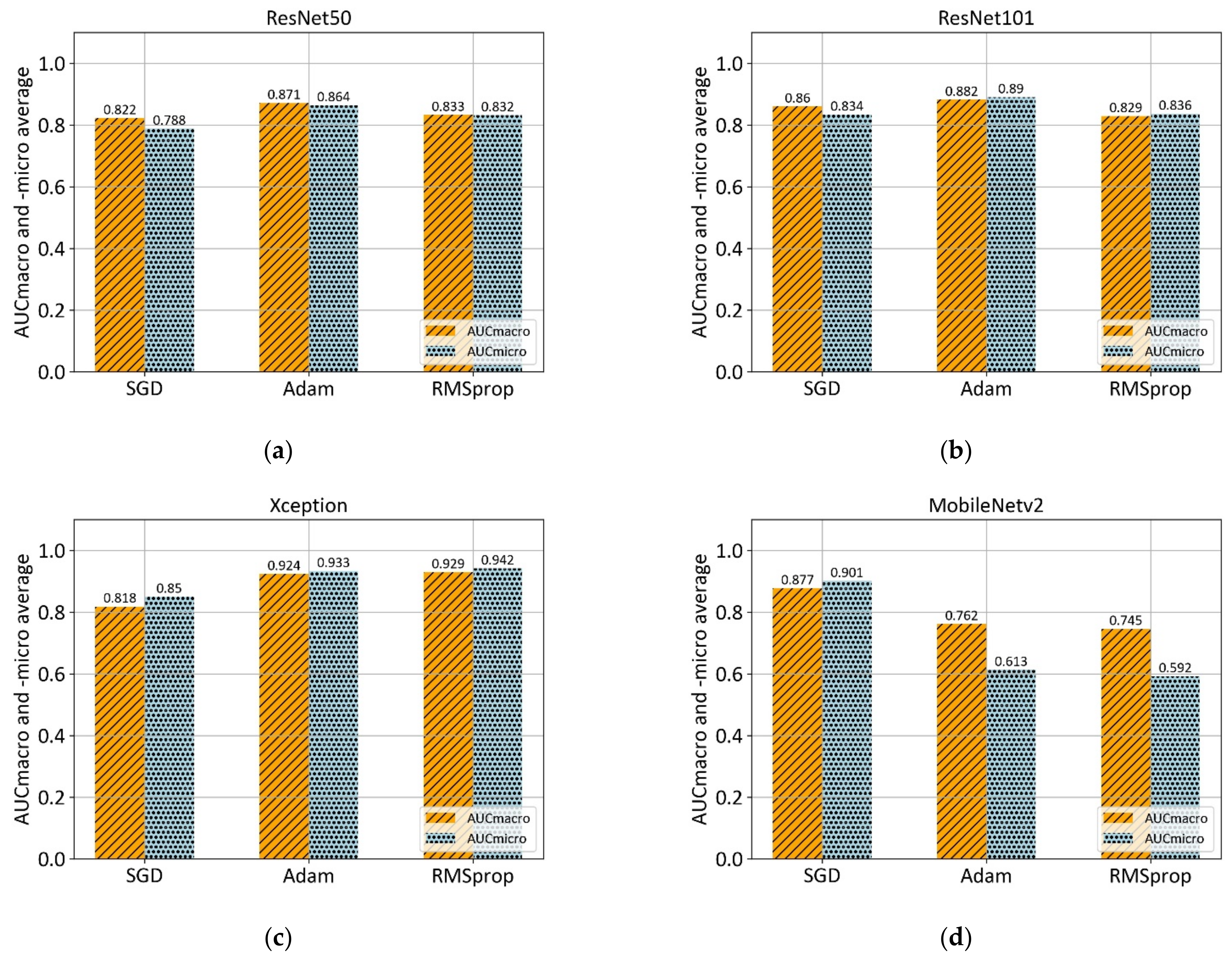
3. Results
4. Discussion
5. Conclusions
Supplementary Materials
Author Contributions
Funding
Institutional Review Board Statement
Informed Consent Statement
Data Availability Statement
Acknowledgments
Conflicts of Interest
References
- Torre, L.A.; Siegel, R.L.; Ward, E.M.; Jemal, A. Global Cancer Incidence and Mortality Rates and Trends—An Update. Cancer Epidemiol. Biomark. Prev. 2015, 25, 16–27. [Google Scholar] [CrossRef] [PubMed]
- Marur, S.; Forastiere, A.A. Head and Neck Cancer: Changing Epidemiology, Diagnosis, and Treatment. Mayo Clin. Proc. 2008, 83, 489–501. [Google Scholar] [CrossRef] [PubMed]
- Sung, H.; Ferlay, J.; Siegel, R.L.; Laversanne, M.; Soerjomataram, I.; Jemal, A.; Bray, F. Global cancer statistics 2020: GLOBOCAN estimates of incidence and mortality worldwide for 36 cancers in 185 countries. Cancer J. Clin. 2021. [Google Scholar] [CrossRef] [PubMed]
- Bagan, J.; Sarrion, G.; Jimenez, Y. Oral cancer: Clinical features. Oral Oncol. 2010, 46, 414–417. [Google Scholar] [CrossRef]
- Ganesh, D.; Sreenivasan, P.; Öhman, J.; Wallström, M.; Braz-Silva, P.H.; Giglio, D.; Kjeller, G.; Hasséus, B. Potentially Malignant Oral Disorders and Cancer Transformation. Anticancer Res. 2018, 38, 3223–3229. [Google Scholar] [CrossRef]
- Ettinger, K.S.; Ganry, L.; Fernandes, R.P. Oral Cavity Cancer. Oral Maxillofac. Surg. Clin. N. Am. 2019, 31, 13–29. [Google Scholar] [CrossRef]
- Milas, Z.L.; Shellenberger, T.D. The Head and Neck Cancer Patient: Neoplasm Management. Oral Maxillofac. Surg. Clin. N. Am. 2019, 31. [Google Scholar] [CrossRef]
- Warnakulasuriya, S.; Reibel, J.; Bouquot, J.; Dabelsteen, E. Oral epithelial dysplasia classification systems: Predictive value, utility, weaknesses and scope for improvement. J. Oral Pathol. Med. 2008, 37, 127–133. [Google Scholar] [CrossRef]
- Mehlum, C.S.; Larsen, S.R.; Kiss, K.; Groentved, A.M.; Kjaergaard, T.; Möller, S.; Godballe, C. Laryngeal precursor lesions: Interrater and intrarater reliability of histopathological assessment. Laryngoscope 2018, 128, 2375–2379. [Google Scholar] [CrossRef]
- Chen, H.; Sung, J.J.Y. Potentials of AI in medical image analysis in Gastroenterology and Hepatology. J. Gastroenterol. Hepatol. 2021, 36, 31–38. [Google Scholar] [CrossRef]
- Stolte, S.; Fang, R. A survey on medical image analysis in diabetic retinopathy. Med Image Anal. 2020, 64, 101742. [Google Scholar] [CrossRef]
- Litjens, G.; Kooi, T.; Bejnordi, B.E.; Setio, A.A.A.; Ciompi, F.; Ghafoorian, M.; van der Laak, J.A.; van Ginneken, B.; Sánchez, C.I. A survey on deep learning in medical image analysis. Med Image Anal. 2017, 42, 60–88. [Google Scholar] [CrossRef]
- Singh, A.; Sengupta, S.; Lakshminarayanan, V. Explainable Deep Learning Models in Medical Image Analysis. J. Imaging 2020, 6, 52. [Google Scholar] [CrossRef]
- Haefner, N.; Wincent, J.; Parida, V.; Gassmann, O. Artificial intelligence and innovation management: A review, framework, and research agenda. Technol. Forecast. Soc. Chang. 2021, 162, 120392. [Google Scholar] [CrossRef]
- Kaba, K.; Sarıgül, M.; Avcı, M.; Kandırmaz, H.M. Estimation of daily global solar radiation using deep learning model. Energy 2018, 162, 126–135. [Google Scholar] [CrossRef]
- Lorencin, I.; Anđelić, N.; Mrzljak, V.; Car, Z. Genetic Algorithm Approach to Design of Multi-Layer Perceptron for Combined Cycle Power Plant Electrical Power Output Estimation. Energies 2019, 12, 4352. [Google Scholar] [CrossRef]
- Gurcan, M.N.; Boucheron, L.E.; Can, A.; Madabhushi, A.; Rajpoot, N.M.; Yener, B. Histopathological Image Analysis: A Review. IEEE Rev. Biomed. Eng. 2009, 2, 147–171. [Google Scholar] [CrossRef]
- Sharma, S.; Mehra, R. Conventional Machine Learning and Deep Learning Approach for Multi-Classification of Breast Cancer Histopathology Images—A Comparative Insight. J. Digit. Imaging 2020, 33, 632–654. [Google Scholar] [CrossRef]
- Wu, Z.; Wang, L.; Li, C.; Cai, Y.; Liang, Y.; Mo, X.; Lu, Q.; Dong, L.; Liu, Y. DeepLRHE: A Deep Convolutional Neural Network Framework to Evaluate the Risk of Lung Cancer Recurrence and Metastasis from Histopathology Images. Front. Genet. 2020, 11, 768. [Google Scholar] [CrossRef]
- Tabibu, S.; Vinod, P.K.; Jawahar, C.V. Pan-Renal Cell Carcinoma classification and survival prediction from histopathology images using deep learning. Sci. Rep. 2019, 9, 1–9. [Google Scholar] [CrossRef]
- Ariji, Y.; Fukuda, M.; Kise, Y.; Nozawa, M.; Yanashita, Y.; Fujita, H.; Katsumata, A.; Ariji, E. Contrast-enhanced computed tomography image assessment of cervical lymph node metastasis in patients with oral cancer by using a deep learning system of artificial intelligence. Oral Surg. Oral Med. Oral Pathol. Oral Radiol. 2019, 127, 458–463. [Google Scholar] [CrossRef]
- Halicek, M.; Dormer, J.D.; Little, J.V.; Chen, A.Y.; Myers, L.; Sumer, B.D.; Fei, B. Hyperspectral Imaging of Head and Neck Squamous Cell Carcinoma for Cancer Margin Detection in Surgical Specimens from 102 Patients Using Deep Learning. Cancers 2019, 11, 1367. [Google Scholar] [CrossRef]
- Horie, Y.; Yoshio, T.; Aoyama, K.; Yoshimizu, S.; Horiuchi, Y.; Ishiyama, A.; Hirasawa, T.; Tsuchida, T.; Ozawa, T.; Ishihara, S.; et al. Diagnostic outcomes of esophageal cancer by artificial intelligence using convolutional neural networks. Gastrointest. Endosc. 2019, 89, 25–32. [Google Scholar] [CrossRef]
- Tamashiro, A.; Yoshio, T.; Ishiyama, A.; Tsuchida, T.; Hijikata, K.; Yoshimizu, S.; Horiuchi, Y.; Hirasawa, T.; Seto, A.; Sasaki, T.; et al. Artificial intelligence-based detection of pharyngeal cancer using convolutional neural networks. Dig. Endosc. 2020, 32, 1057–1065. [Google Scholar] [CrossRef]
- Jeyaraj, P.R.; Nadar, E.R.S. Computer-assisted medical image classification for early diagnosis of oral cancer employing deep learning algorithm. J. Cancer Res. Clin. Oncol. 2019, 145, 829–837. [Google Scholar] [CrossRef]
- Bhandari, B.; Alsadoon, A.; Prasad, P.W.C.; Abdullah, S.; Haddad, S. Deep learning neural network for texture feature extraction in oral cancer: Enhanced loss function. Multimed. Tools Appl. 2020, 79, 1–24. [Google Scholar] [CrossRef]
- Xu, S.; Liu, Y.; Hu, W.; Zhang, C.; Liu, C.; Zong, Y.; Chen, S.; Lu, Y.; Yang, L.; Ng, E.Y.K.; et al. An Early Diagnosis of Oral Cancer based on Three-Dimensional Convolutional Neural Networks. IEEE Access 2019, 7, 158603–158611. [Google Scholar] [CrossRef]
- Welikala, R.A.; Remagnino, P.; Lim, J.H.; Chan, C.S.; Rajendran, S.; Kallarakkal, T.G.; Zain, R.B.; Jayasinghe, R.D.; Rimal, J.; Kerr, A.R.; et al. Automated Detection and Classification of Oral Lesions Using Deep Learning for Early Detection of Oral Cancer. IEEE Access 2020, 8, 132677–132693. [Google Scholar] [CrossRef]
- Chan, C.-H.; Huang, T.-T.; Chen, C.-Y.; Lee, C.-C.; Chan, M.-Y.; Chung, P.-C. Texture-Map-Based Branch-Collaborative Network for Oral Cancer Detection. IEEE Trans. Biomed. Circuits Syst. 2019, 13, 766–780. [Google Scholar] [CrossRef] [PubMed]
- Fraz, M.M.; Khurram, S.A.; Graham, S.; Shaban, M.; Hassan, M.; Loya, A.; Rajpoot, N.M. FABnet: Feature attention-based network for simultaneous segmentation of microvessels and nerves in routine histology images of oral cancer. Neural Comput. Appl. 2020, 32, 9915–9928. [Google Scholar] [CrossRef]
- Das, N.; Hussain, E.; Mahanta, L.B. Automated classification of cells into multiple classes in epithelial tissue of oral squamous cell carcinoma using transfer learning and convolutional neural network. Neural Netw. 2020, 128, 47–60. [Google Scholar] [CrossRef]
- El-Naggar, A.K.; Chan, J.K.; Takata, T.; Grandis, J.R.; Slootweg, P.J. WHO classification of head and neck tumours. Int. Agency Res. Cancer 2017. [Google Scholar] [CrossRef]
- Amin, M.B.; Edge, S.B.; Greene, F.L.; Byrd, D.R.; Brookland, R.K.; Washington, M.K.; Gershenwald, J.E.; Compton, C.C.; Hess, K.R.; Sullivan, D.C.; et al. AJCC Cancer Staging Manual, 8th ed.; Springer: Cham, Switzerland, 2017. [Google Scholar] [CrossRef]
- Jakovac, H.; Stašić, N.; Krašević, M.; Jonjić, N.; Radošević-Stašić, B. Expression profiles of metallothionein-I/II and megalin/LRP-2 in uterine cervical squamous lesions. Virchows Archiv 2021, 478, 735–746. [Google Scholar] [CrossRef]
- Shorten, C.; Khoshgoftaar, T.M. A survey on Image Data Augmentation for Deep Learning. J. Big Data 2019, 6, 60. [Google Scholar] [CrossRef]
- Han, J.; Kamber, M.; Pei, J. Classification. In Data Mining; Elsevier: Amsterdam, The Netherlands, 2012; pp. 327–391. [Google Scholar]
- Addison, P.S. The Illustrated Wavelet Transform Handbook: Introductory Theory and Applications in Science, Engineering, Medicine and Finance; CRC Press: Boca Raton, FL, USA, 2017. [Google Scholar] [CrossRef]
- Štifanić, D.; Musulin, J.; Miočević, A.; Šegota, S.B.; Šubić, R.; Car, Z. Impact of COVID-19 on Forecasting Stock Prices: An Integration of Stationary Wavelet Transform and Bidirectional Long Short-Term Memory. Complexity 2020, 2020, 1–12. [Google Scholar] [CrossRef]
- Zhang, D. Wavelet transform. In Fundamentals of Image Data Mining; Springer: Cham, Switzerland, 2019; pp. 35–44. [Google Scholar] [CrossRef]
- Qayyum, H.; Majid, M.; Anwar, S.M.; Khan, B. Facial Expression Recognition Using Stationary Wavelet Transform Features. Math. Probl. Eng. 2017, 2017, 1–9. [Google Scholar] [CrossRef]
- Janani, S.; Marisuganya, R.; Nivedha, R. MRI image segmentation using Stationary Wavelet Transform and FCM algorithm. Int. J. Comput. Appl. 2013. [Google Scholar] [CrossRef]
- Feurer, M.; Hutter, F. Hyperparameter optimization. In Automated Machine Learning; Springer: Cham, Switzerland, 2019; pp. 3–33. [Google Scholar] [CrossRef]
- Swersky, K.; Snoek, J.; Adams, R.P. Multi-task Bayesian optimization. In NIPS’13: Proceedings of the 26th International Conference on Neural Information Processing Systems 2004–2012; Curran Associates Inc.: Red Hook, NY, USA, 2013. [Google Scholar]
- Chollet, F. Xception: Deep Learning with Depthwise Separable Convolutions. In Proceedings of the IEEE Conference on Computer Vision and Pattern Recognition (CVPR), Honolulu, HI, USA, 21–26 July 2017; pp. 1251–1258. [Google Scholar]
- He, K.; Zhang, X.; Ren, S.; Sun, J. Deep residual learning for image recognition. In Proceedings of the IEEE Conference on Computer Vision and Pattern Recognition, Las Vegas, NV, USA, 27–30 June 2016; pp. 770–778. [Google Scholar] [CrossRef]
- Sandler, M.; Howard, A.; Zhu, M.; Zhmoginov, A.; Chen, L.-C. MobileNetV2: Inverted Residuals and Linear Bottlenecks. In Proceedings of the 2018 IEEE/CVF Conference on Computer Vision and Pattern Recognition, Salt Lake City, UT, USA, 18–23 June 2018; pp. 4510–4520. [Google Scholar]
- Chen, L.-C.; Papandreou, G.; Kokkinos, I.; Murphy, K.; Yuille, A.L. DeepLab: Semantic Image Segmentation with Deep Convolutional Nets, Atrous Convolution, and Fully Connected CRFs. IEEE Trans. Pattern Anal. Mach. Intell. 2017, 40, 834–848. [Google Scholar] [CrossRef]
- Chen, L.C.; Papandreou, G.; Schroff, F.; Adam, H. Rethinking atrous convolution for semantic image segmentation. arXiv 2017, arXiv:1706.05587. [Google Scholar]
- Chen, L.C.; Zhu, Y.; Papandreou, G.; Schroff, F.; Adam, H. Encoder-decoder with atrous separable convolution for semantic image segmentation. In Proceedings of the European Conference on Computer Vision (ECCV), Munich, Germany, 8–14 September 2018; pp. 801–818. [Google Scholar] [CrossRef]
- Choudhury, A.R.; Vanguri, R.; Jambawalikar, S.R.; Kumar, P. Segmentation of brain tumors using DeepLabv3+. In International MICCAI Brainlesion Workshop; Springer: Cham, Switzerland, 2018; pp. 154–167. [Google Scholar] [CrossRef]
- Tharwat, A. Classification assessment methods. Appl. Comput. Inform. 2020, 17, 168–192. [Google Scholar] [CrossRef]
- Leonard, L. Web-Based Behavioral Modeling for Continuous User Authentication (CUA). In Advances in Computers; Elsevier: Amsterdam, The Netherlands, 2017; Volume 105, pp. 1–44. [Google Scholar]
- Rezatofighi, H.; Tsoi, N.; Gwak, J.; Sadeghian, A.; Reid, I.; Savarese, S. Generalized Intersection Over Union: A Metric and a Loss for Bounding Box Regression. In Proceedings of the 2019 IEEE/CVF Conference on Computer Vision and Pattern Recognition (CVPR), Long Beach, CA, USA, 15–20 June 2019; pp. 658–666. [Google Scholar]
- Chicco, D.; Jurman, G. The advantages of the Matthews correlation coefficient (MCC) over F1 score and accuracy in binary classification evaluation. BMC Genom. 2020, 21, 6. [Google Scholar] [CrossRef]
- Gunawardana, A.; Shani, G. A survey of accuracy evaluation metrics of recommendation tasks. J. Mach. Learn. Res. 2009, 10. [Google Scholar] [CrossRef]
- Mumtaz, W.; Ali, S.S.A.; Yasin, M.A.M.; Malik, A.S. A machine learning framework involving EEG-based functional connectivity to diagnose major depressive disorder (MDD). Med Biol. Eng. Comput. 2018, 56, 233–246. [Google Scholar] [CrossRef]
- Speight, P.M.; Farthing, P.M. The pathology of oral cancer. Br. Dent. J. 2018, 225, 841–847. [Google Scholar] [CrossRef]
- Li, L.; Pan, X.; Yang, H.; Liu, Z.; He, Y.; Li, Z.; Fan, Y.; Cao, Z.; Zhang, L. Multi-task deep learning for fine-grained classification and grading in breast cancer histopathological images. Multimed. Tools Appl. 2018, 79, 14509–14528. [Google Scholar] [CrossRef]
- Al-Milaji, Z.; Ersoy, I.; Hafiane, A.; Palaniappan, K.; Bunyak, F. Integrating segmentation with deep learning for enhanced classification of epithelial and stromal tissues in H&E images. Pattern Recognit. Lett. 2019, 119, 214–221. [Google Scholar] [CrossRef]
- Almangush, A.; Mäkitie, A.A.; Triantafyllou, A.; de Bree, R.; Strojan, P.; Rinaldo, A.; Hernandez-Prera, J.C.; Suárez, C.; Kowalski, L.P.; Ferlito, A.; et al. Staging and grading of oral squamous cell carcinoma: An update. Oral Oncol. 2020, 107, 104799. [Google Scholar] [CrossRef]
- Mascitti, M.; Zhurakivska, K.; Togni, L.; Caponio, V.C.A.; Almangush, A.; Balercia, P.; Balercia, A.; Rubini, C.; Muzio, L.L.; Santarelli, A.; et al. Addition of the tumour–stroma ratio to the 8th edition American Joint Committee on Cancer staging system improves survival prediction for patients with oral tongue squamous cell carcinoma. Histopathology 2020, 77, 810–822. [Google Scholar] [CrossRef]
- Heikkinen, I.; Bello, I.O.; Wahab, A.; Hagström, J.; Haglund, C.; Coletta, R.D.; Nieminen, P.; Mäkitie, A.A.; Salo, T.; Leivo, I.; et al. Assessment of Tumor-infiltrating Lymphocytes Predicts the Behavior of Early-stage Oral Tongue Cancer. Am. J. Surg. Pathol. 2019, 43, 1392–1396. [Google Scholar] [CrossRef]
- Agarwal, R.; Chaudhary, M.; Bohra, S.; Bajaj, S. Evaluation of natural killer cell (CD57) as a prognostic marker in oral squamous cell carcinoma: An immunohistochemistry study. J. Oral Maxillofac. Pathol. 2016, 20, 173–177. [Google Scholar] [CrossRef]
- Fang, J.; Li, X.; Ma, D.; Liu, X.; Chen, Y.; Wang, Y.; Lui, V.W.Y.; Xia, J.; Cheng, B.; Wang, Z. Prognostic significance of tumor infiltrating immune cells in oral squamous cell carcinoma. BMC Cancer 2017, 17, 375. [Google Scholar] [CrossRef] [PubMed]
- Jonnalagedda, P.; Schmolze, D.; Bhanu, B. mvpnets: Multi-viewing path deep learning neural networks for magnification invariant diagnosis in breast cancer. In Proceedings of the 2018 IEEE 18th International Conference on Bioinformatics and Bioengineering (BIBE), Taichung, Taiwan, 29–31 October 2018; pp. 189–194. [Google Scholar] [CrossRef]
- Silva, A.B.; Martins, A.S.; Neves, L.A.; Faria, P.R.; Tosta, T.A.; do Nascimento, M.Z. Automated nuclei segmentation in dysplastic histopathological oral tissues using deep neural networks. In Iberoamerican Congress on Pattern Recognition; Springer: Cham, Switzerland, 2019; pp. 365–374. [Google Scholar] [CrossRef]
- Fauzi, M.F.A.; Chen, W.; Knight, D.; Hampel, H.; Frankel, W.L.; Gurcan, M.N. Tumor Budding Detection System in Whole Slide Pathology Images. J. Med. Syst. 2019, 44, 38. [Google Scholar] [CrossRef] [PubMed]
- Rashmi, R.; Prasad, K.; Udupa CB, K.; Shwetha, V. A Comparative Evaluation of Texture Features for Semantic Segmentation of Breast Histopathological Images. IEEE Access 2020, 8, 64331–64346. [Google Scholar] [CrossRef]


| Characteristic of the Patients | % | |
|---|---|---|
| Sex | F | 35 |
| M | 65 | |
| Age | To 49 | 6 |
| 50–59 | 13 | |
| 60–69 | 58 | |
| +70 | 23 | |
| Smoking | Y | 69 |
| N | 31 | |
| Lymph Node Metastases | Y | 46 |
| N | 54 | |
| Histological Grade (G) | I | 50 |
| II | 33 | |
| III | 17 |
| Hyperparameter | Possible Parameters |
|---|---|
| a | 0–0.1 |
| b | 0–0.1 |
| c | 0–0.1 |
| d | 0.001–1 |
| Wavelet function | Haar, sym2, db2, bior1.3 |
| Layer | Output | Layers | ResNet50 | ResNet101 |
|---|---|---|---|---|
| Number of Repeating Layers | ||||
| Conv1 | 112 × 112 | 7 × 7, 64, stride 2 | ×1 | ×1 |
| 3 × 3 max pool, stride 2 | ×1 | ×1 | ||
| Conv2_x | 56 × 56 | 1 × 1, 64 | ×3 | ×3 |
| 3 × 3, 64 | ||||
| 1 × 1, 256 | ||||
| Conv3_x | 28 × 28 | 1 × 1, 128 | ×4 | ×4 |
| 3 × 3, 128 | ||||
| 1 × 1, 512 | ||||
| Conv4_x | 14 × 14 | 1 × 1, 256 | ×6 | ×23 |
| 3 × 3, 256 | ||||
| 1 × 1, 1024 | ||||
| Conv5_x | 7 × 7 | 1 × 1, 512 | ×3 | ×3 |
| 3 × 3, 512 | ||||
| 1 × 1, 2048 | ||||
| 1 × 1 | Flatten | ×1 | ×1 | |
| 3-d Fully Connected | ||||
| Softmax | ||||
| Input | Operator | Expansion Factor (t) | Number of Output Channels (c) | Repeating Number (n) | Stride (s) |
|---|---|---|---|---|---|
| 224 × 224 × 3 | conv2d | - | 32 | 1 | 2 |
| 112 × 112 × 32 | bottleneck | 1 | 16 | 1 | 1 |
| 112 × 112 × 16 | bottleneck | 6 | 24 | 2 | 2 |
| 56 × 56 × 24 | bottleneck | 6 | 32 | 3 | 2 |
| 28 × 28 × 32 | bottleneck | 6 | 64 | 4 | 2 |
| 14 × 14 × 64 | bottleneck | 6 | 96 | 3 | 1 |
| 14 × 14 × 96 | bottleneck | 6 | 160 | 3 | 2 |
| 7 × 7 × 160 | bottleneck | 6 | 320 | 1 | 1 |
| 7 × 7 × 320 | conv2d 1 × 1 | - | 1280 | 1 | 1 |
| 7 × 7 × 1280 | avgpool 7 × 7 | - | - | 1 | - |
| 1 × 1 × 1280 | fully connected (Softmax) | - | 3 | - |
| Algorithm | AUCmacro ± σ | AUCmicro ± σ |
|---|---|---|
| ResNet50 | 0.871 ± 0.105 | 0.864 ± 0.090 |
| ResNet101 | 0.882 ± 0.125 | 0.890 ± 0.112 |
| Xception | 0.929 ± 0.087 | 0.942 ± 0.074 |
| MobileNetv2 | 0.877 ± 0.062 | 0.900 ± 0.049 |
| Parameters | Xception + SWT | |||||
|---|---|---|---|---|---|---|
| a | b | c | d | Wavelet | AUCmacro ± σ | AUCmicro ± σ |
| 0.0084 | 0.0713 | 0.0599 | 0.0566 | sym2 | 0.956 ± 0.054 | 0.964 ± 0.040 |
| 0.0091 | 0.0301 | 0.0086 | 0.3444 | db2 | 0.963 ± 0.042 | 0.966 ± 0.027 |
| 0.0063 | 0.0021 | 0.0771 | 0.3007 | db2 | 0.947 ± 0.092 | 0.954 ± 0.069 |
| 0.0081 | 0.0933 | 0.0469 | 0.2520 | haar | 0.952 ± 0.056 | 0.958 ± 0.050 |
| 0.0053 | 0.0575 | 0.0649 | 0.1694 | bior1.3 | 0.962 ± 0.050 | 0.965 ± 0.046 |
| mIOU ± σ | F1 ± σ | Accuracy ± σ | Precision ± σ | Sensitivity ± σ | Specificity ± σ | ||
|---|---|---|---|---|---|---|---|
| DeepLabv3+ & Xception_65 | Original | 0.864 ± 0.020 | 0.933 ± 0.058 | 0.934 ± 0.012 | 0.933 ± 0.019 | 0.967 ± 0.013 | 0.873 ± 0.017 |
| sym2 | 0.874 ± 0.037 | 0.953 ± 0.016 | 0.939 ± 0.019 | 0.950 ± 0.025 | 0.956 ± 0.012 | 0.908 ± 0.040 | |
| db2 | 0.876 ± 0.032 | 0.953 ± 0.016 | 0.940 ± 0.017 | 0.952 ± 0.019 | 0.955 ± 0.014 | 0.911 ± 0.031 | |
| Haar | 0.879 ± 0.027 | 0.955 ± 0.014 | 0.941 ± 0.015 | 0.951 ± 0.018 | 0.958 ± 0.016 | 0.910 ± 0.026 | |
| bior1.3 | 0.874 ± 0.030 | 0.953 ± 0.015 | 0.939 ± 0.016 | 0.948 ± 0.020 | 0.958 ± 0.021 | 0.904 ± 0.027 |
Publisher’s Note: MDPI stays neutral with regard to jurisdictional claims in published maps and institutional affiliations. |
© 2021 by the authors. Licensee MDPI, Basel, Switzerland. This article is an open access article distributed under the terms and conditions of the Creative Commons Attribution (CC BY) license (https://creativecommons.org/licenses/by/4.0/).
Share and Cite
Musulin, J.; Štifanić, D.; Zulijani, A.; Ćabov, T.; Dekanić, A.; Car, Z. An Enhanced Histopathology Analysis: An AI-Based System for Multiclass Grading of Oral Squamous Cell Carcinoma and Segmenting of Epithelial and Stromal Tissue. Cancers 2021, 13, 1784. https://doi.org/10.3390/cancers13081784
Musulin J, Štifanić D, Zulijani A, Ćabov T, Dekanić A, Car Z. An Enhanced Histopathology Analysis: An AI-Based System for Multiclass Grading of Oral Squamous Cell Carcinoma and Segmenting of Epithelial and Stromal Tissue. Cancers. 2021; 13(8):1784. https://doi.org/10.3390/cancers13081784
Chicago/Turabian StyleMusulin, Jelena, Daniel Štifanić, Ana Zulijani, Tomislav Ćabov, Andrea Dekanić, and Zlatan Car. 2021. "An Enhanced Histopathology Analysis: An AI-Based System for Multiclass Grading of Oral Squamous Cell Carcinoma and Segmenting of Epithelial and Stromal Tissue" Cancers 13, no. 8: 1784. https://doi.org/10.3390/cancers13081784
APA StyleMusulin, J., Štifanić, D., Zulijani, A., Ćabov, T., Dekanić, A., & Car, Z. (2021). An Enhanced Histopathology Analysis: An AI-Based System for Multiclass Grading of Oral Squamous Cell Carcinoma and Segmenting of Epithelial and Stromal Tissue. Cancers, 13(8), 1784. https://doi.org/10.3390/cancers13081784