1. Introduction
Since piezoelectric actuators (PZAs) have the advantages of fast response, high displacement resolution, small size, and simple construction, they are widely used in diverse precision positioning applications at the micro/nano scale, such as optical fiber alignment [
1], medical micromanipulator [
2], micromachining [
3,
4], and vibration control [
5]. However, the hysteresis behavior of PZAs restricts the usefulness of these actuators in precision manipulation applications. Hysteresis is a well-known input/output multi-loop phenomenon that occurs in piezoelectric materials. Its presence is a kind of non-local memory meaning that the response to the input excitation depends not only on the instantaneousness of the input but also its history path [
6]. Therefore, accurate modeling and prediction of hysteresis in piezoelectric actuator are fundamental steps to acquire high performance in precision positioning systems.
A number of hysteresis models for PZAs are available in the literature. These models can be divided into two categories: physical and phenomenological model. Physical models try to describe the hysteresis model through internal mechanisms, the relationship of energy, displacement and so on [
7,
8]. They are based on the physical principles of materials. However, establishing a physical model is difficult since the physical features of a hysteretic system are usually very complicated. Furthermore, the physical model lacks generality. The physical model of one hysteretic system cannot be directly used in another system. Phenomenological models try to describe hysteresis curves by directly using a mathematical model based on experimental data without paying attention to theunderlying physical essence of hysteresis phenomenon. The most widely used phenomenological models are the Preisach model [
9,
10], Prandtl-Ishlinskii model [
11,
12] and Bouc-Wen model [
13]. However, Preisach models need to store a large number of databases and their calculation is bulky. Prandtl-Ishlinskii models are a subclass of Preisachmodels. Although they have fewer data and analytical properties, their accuracy is limited by their symmetric structure. For the Bouc-Wen model, it is hard to achieve high accuracy because of the rigid structure of its governing equation. These models have rigid structures so that the accuracy is limited. To solve this problem, several phenomenological modeling approaches based on empirical observations have been developed recently. Ru and Sun propose a mathematical model based on the similarities of hysteresis curves and the effects of turning points [
14,
15]. Bashash and Jalili disclose and demonstrate the underlying intellectual behavior of hysteresis. Based on this, several memory-based constitutive mathematical modeling frameworks have been developed [
6,
16,
17].However, the calculation is bulky. Nguyen and Choi [
18] store two discretized first-order datasets of ascending and descending curves in advance and then use congruency property to get high-order hysteretic curves. However, this model needs a lot of memory space to store the datasets. Besides, the above mentioned models do not consider dynamic effect. Little research about dynamic empirical models of piezoelectric actuators have been carried out [
19]. In order to solve the problems above, geometric similarity and time-scale similarity of displacement time series were proposed in our previous work [
20]. However, geometric similarity is not applicable for predicting high-order hysteresis behavior.
To predict complex dynamic hysteresis behavior, this study proposes a novel hysteresis model to describe the complex dynamic hysteresis behavior of a piezoelectric actuator. The proposed model is formulated based on the segment-similarities of hysteresis nonlinearity. Segment-similarity describes the similarity relationship between hysteresis curves with different turning points. Time-scale similarity, which describes the relationship between hysteresis curves with different rates, is also used to solve the problem of the hysteresis dynamic. Compared to the Preisach model (which is one of the most widely used phenomenological models and is based on the experimental data of first reversal curves), the formulation procedure of the proposed model is simpler and more straightforward and requires less computation. The experimental results show that the proposed model can produce better hysteresis prediction accuracy than the Preisach model.
The rest of the paper is arranged as follows: the experimental platform is shown in
Section 2.
Section 3 introduces some inherent properties of hysteresis in a PZA. In
Section 4, the segment similarity is proposed to describe the similarity relationship between hysteresis curves with different extremes. Time-scale similarity is used to describe the dynamic behavior. Then, a hysteresis model is established based on the similarities in
Section 5. In
Section 6, the model is tested using different kinds of inputs with multi-amplitude and different rates. The proposed model is also compared with the Preisach model. Finally, the research conclusion is given in
Section 7.
2. Experimental Setup
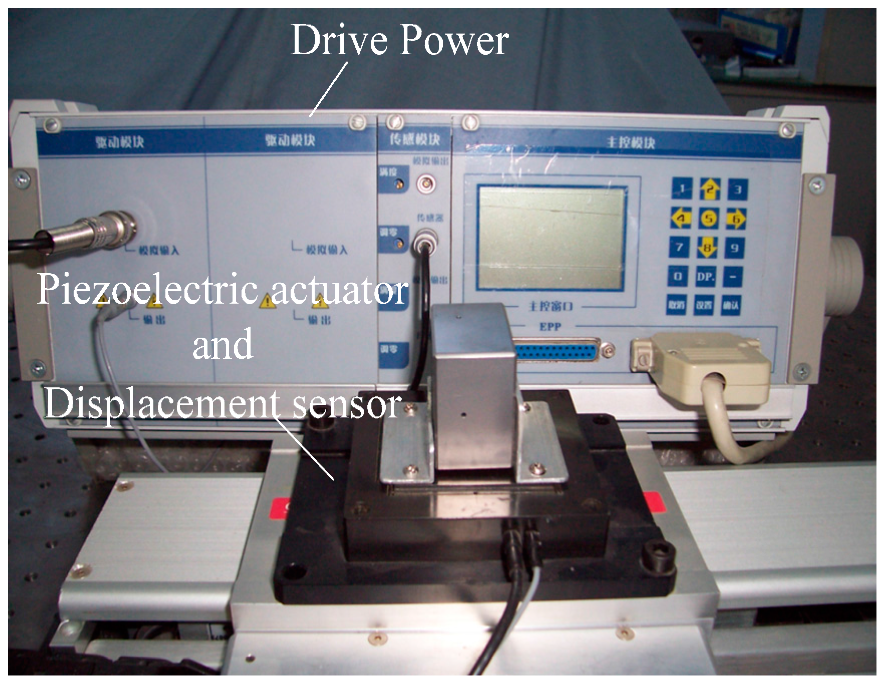
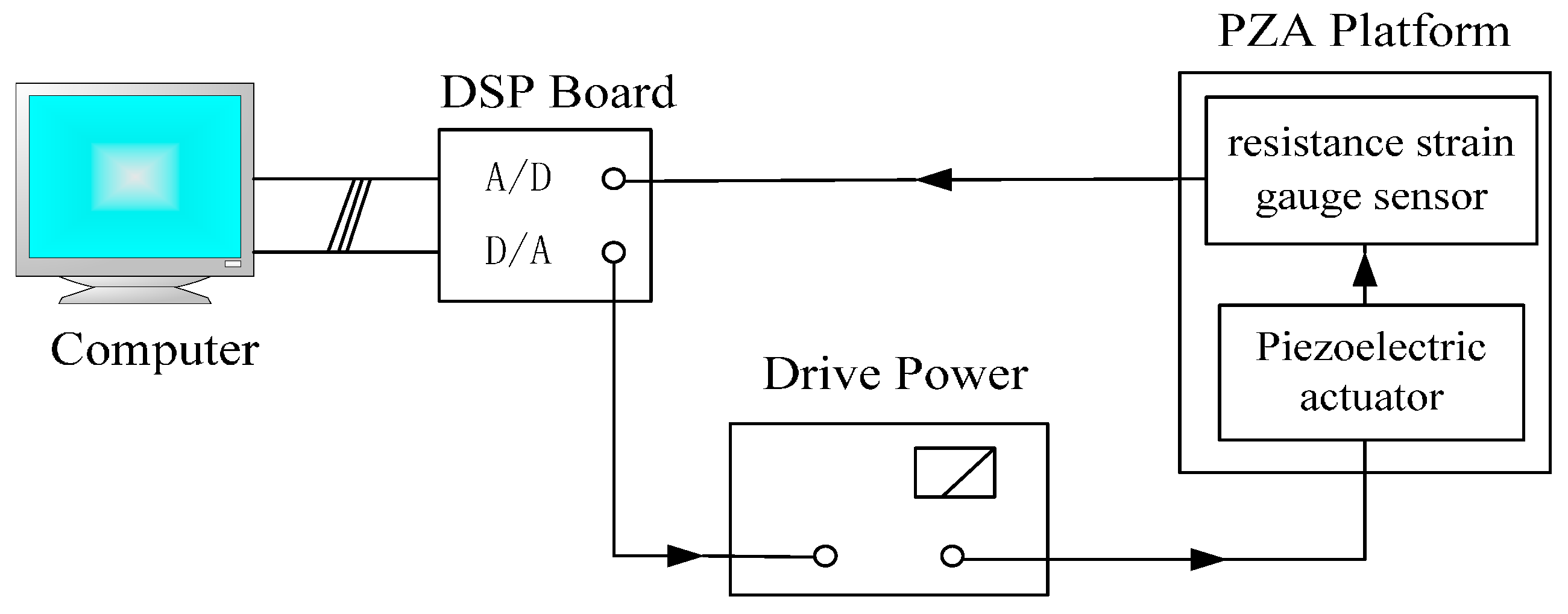
The similarities among hysteresis trajectories are investigated through a set of experimental tests on a piezoelectric actuator-based micro/nano-meter movement platform system as depicted in
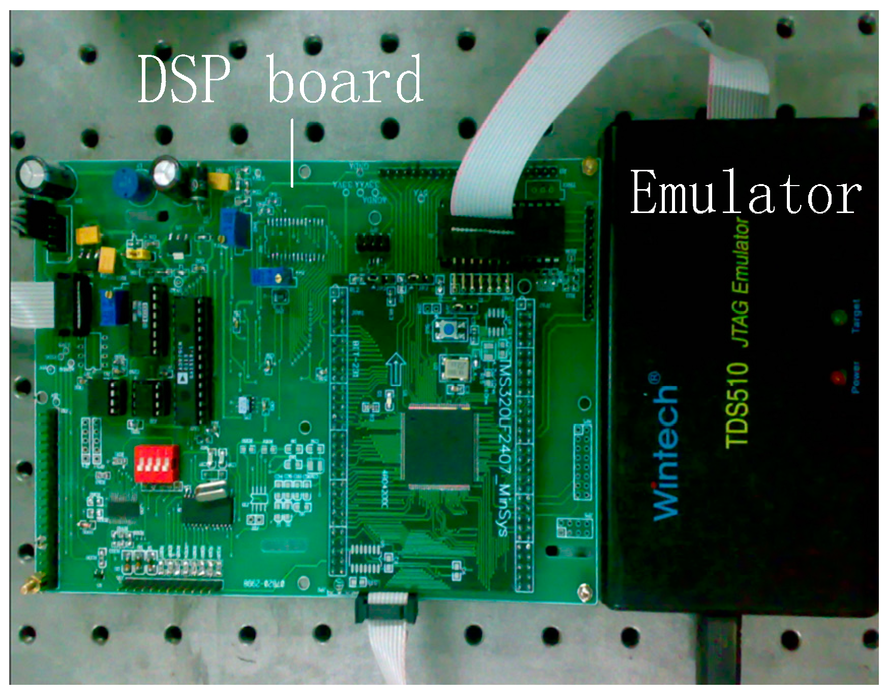
Figure 1. A digital signal processor (DSP, TMS320LF2407, Texas Instruments, Houston, TX, USA) system is employed to implement controller as shown in
Figure 2. The D/A (16-bit AD669, Analog Devices, Norwood, MA, USA) board produces an analogy voltage output which is then amplified by drive power (HPV series) to provide a voltage for driving PZA (MPT-1JRL/I002, Physik Instrumente, Shanghai, China). The output voltages of the power amplifier range from 0 to 150 V, and the resolution is 5 mV. Output displacements of PZA are measured by a resistance strain gauge sensor which is installed within the platform as a micrometer and then are converted into digital signals by A/D (16-bit AD976, Analog Devices, Norwood, MA, USA) board. A serial port is used to pass the data from the DSP to the computer. The devices are shown in
Figure 3. The withstand-voltage range of PZA is −30–120 V. The input voltages of the PZA are limited to the range of 0–100 V, considering the safety margin and the driving ability of the power amplifier.
Figure 1.
The piezoelectric actuator-based experimental system.
Figure 1.
The piezoelectric actuator-based experimental system.
Figure 2.
The controller system.
Figure 2.
The controller system.
Figure 3.
The PZA experiment devices.
Figure 3.
The PZA experiment devices.
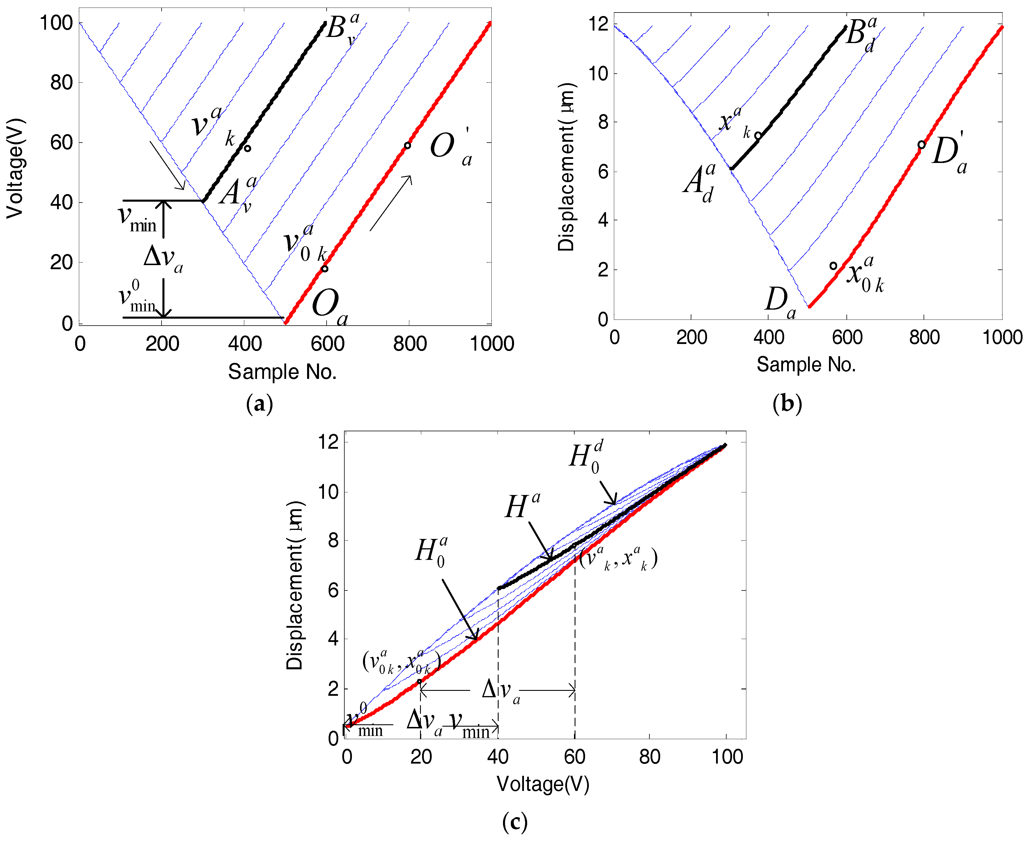
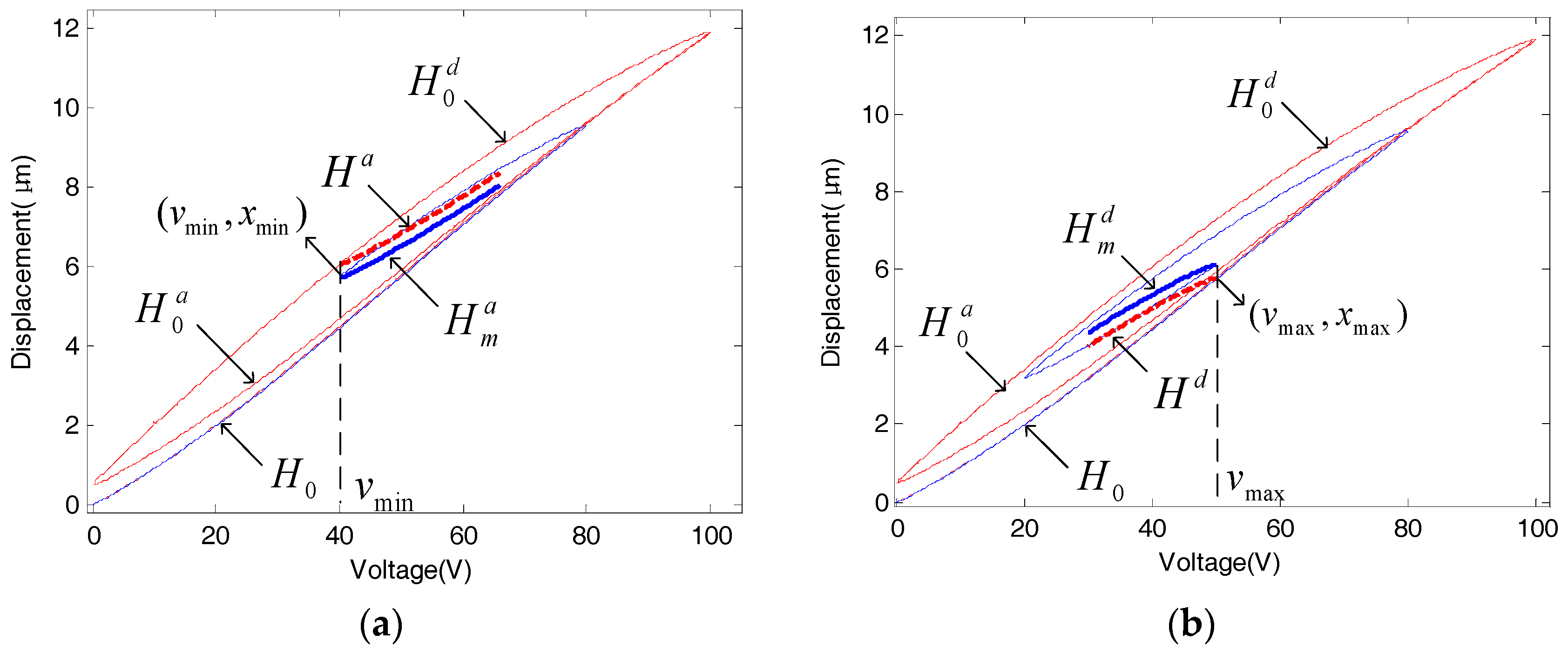
5. Hysteresis Model Formulation
Based on the similarity proposed in
Section 4, the hysteresis model of PZA is formulated in this section. Before implementing the model, the triangular input voltage sequence
(the reference voltage sequence) with the rate of
(that is 10 V/s in this paper), the minimum of
(that is 0 V in this paper), the maximum of
(that is 100 V in this paper), and the corresponding output displacement sequence
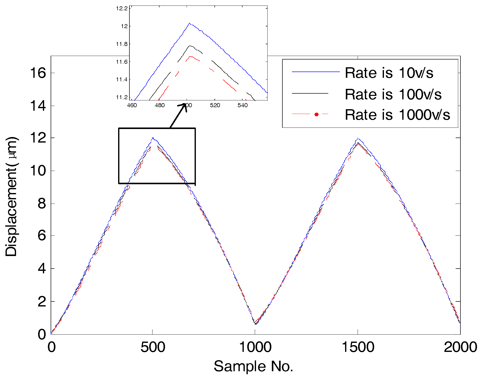
(the reference displacement sequence) need to be identified through experiment in advance. When giving PZA an input excitatio
in any waveforms with a rate of
, the output displacement
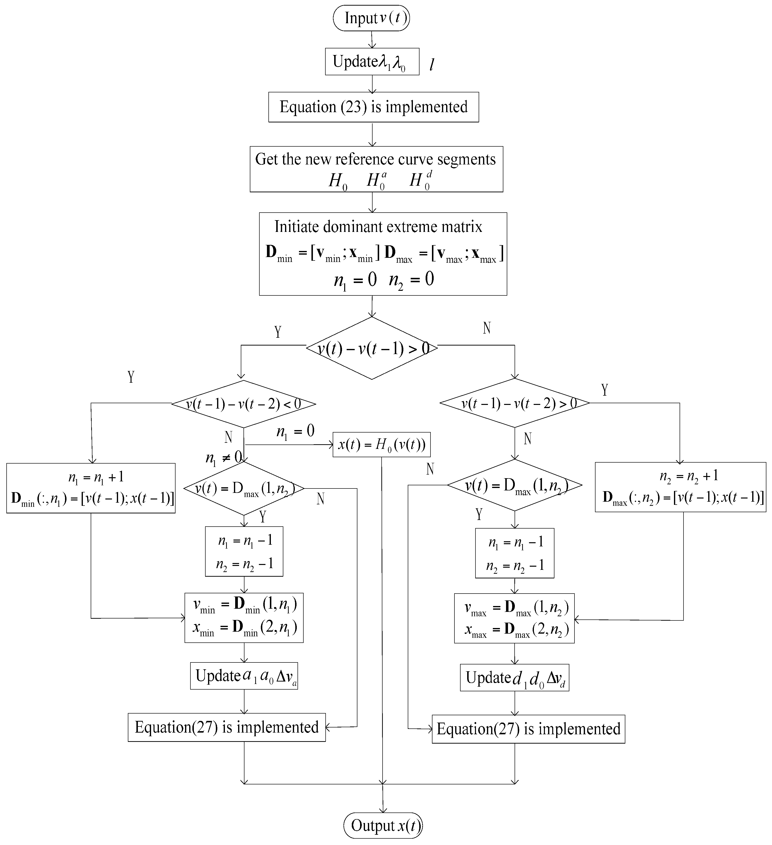
x(t) can be obtained through this proposed model. The procedure for modeling is as follows:
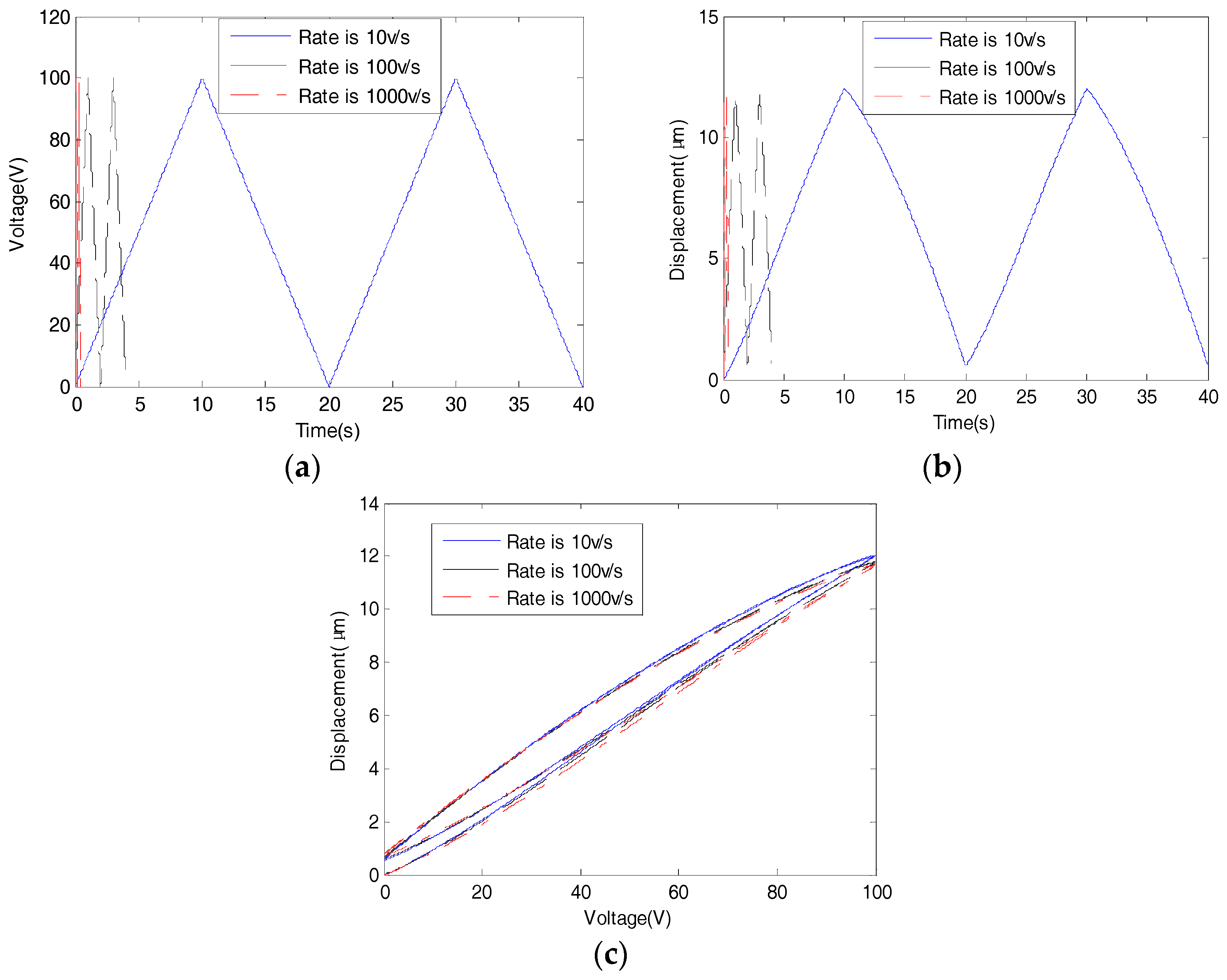
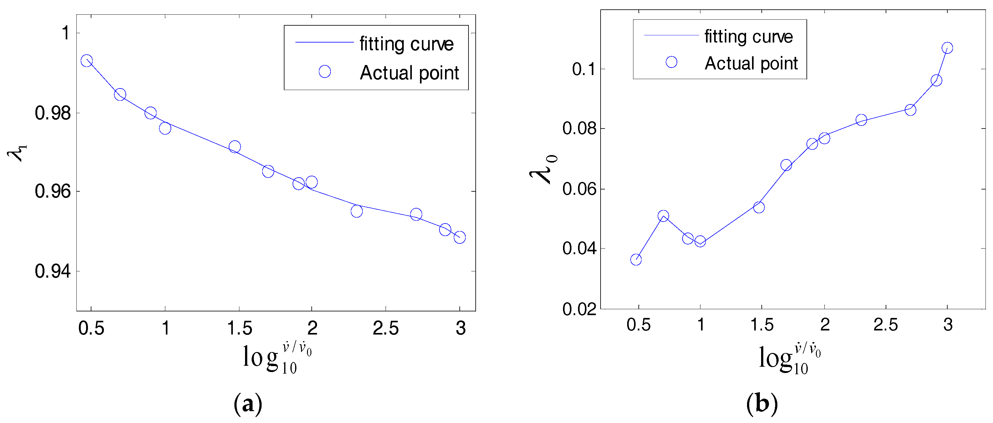
Step1: First, calculate the rate of input voltage according to the amplitude and frequency. The time-scale similarity Equation (23) is implemented to achieve a new reference displacement
sequence with rate of
. If
, updating the similarity factors
,
through Equations (21) and (22). Otherwise,
,
.
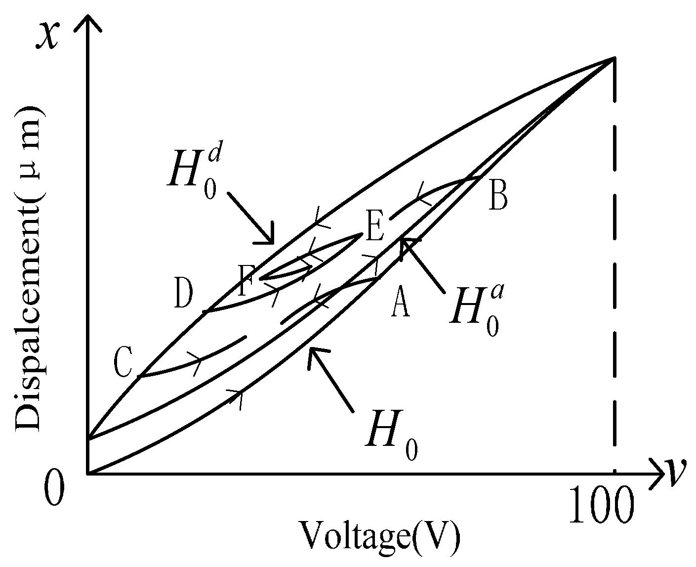
Step 2: The new reference curve segments constituted by the input voltage sequence
and new displacement sequence
are curve-fitted in polynomial forms:
where,
is the first reference ascending hysteresis curve segment that departs from the initial state.
is the second reference ascending hysteresis curve segment that departs from the lower turning point.
is the first reference descending hysteresis curve segment that departs from the upper turning point.
are the coefficients of polynomials.
Step 3: Updating similarity factors
according to the current dominant extreme. If
,
. If
,
. Alternatively, these similarity factors are updated by Equations (5), (6), (12) and (13), respectively. The output displacement
x(t) corresponding to input excitation
v(t) is obtained through Equation (27).
where
is the ascending hysteresis curve segment whose dominant extreme is
.
is the descending hysteresis curve segment whose dominant extreme is
.
The schematic diagram of the modeling is shown in
Figure 16.
Figure 16.
The schematic diagram of the modeling.
Figure 16.
The schematic diagram of the modeling.
6. Experiments and Discussions
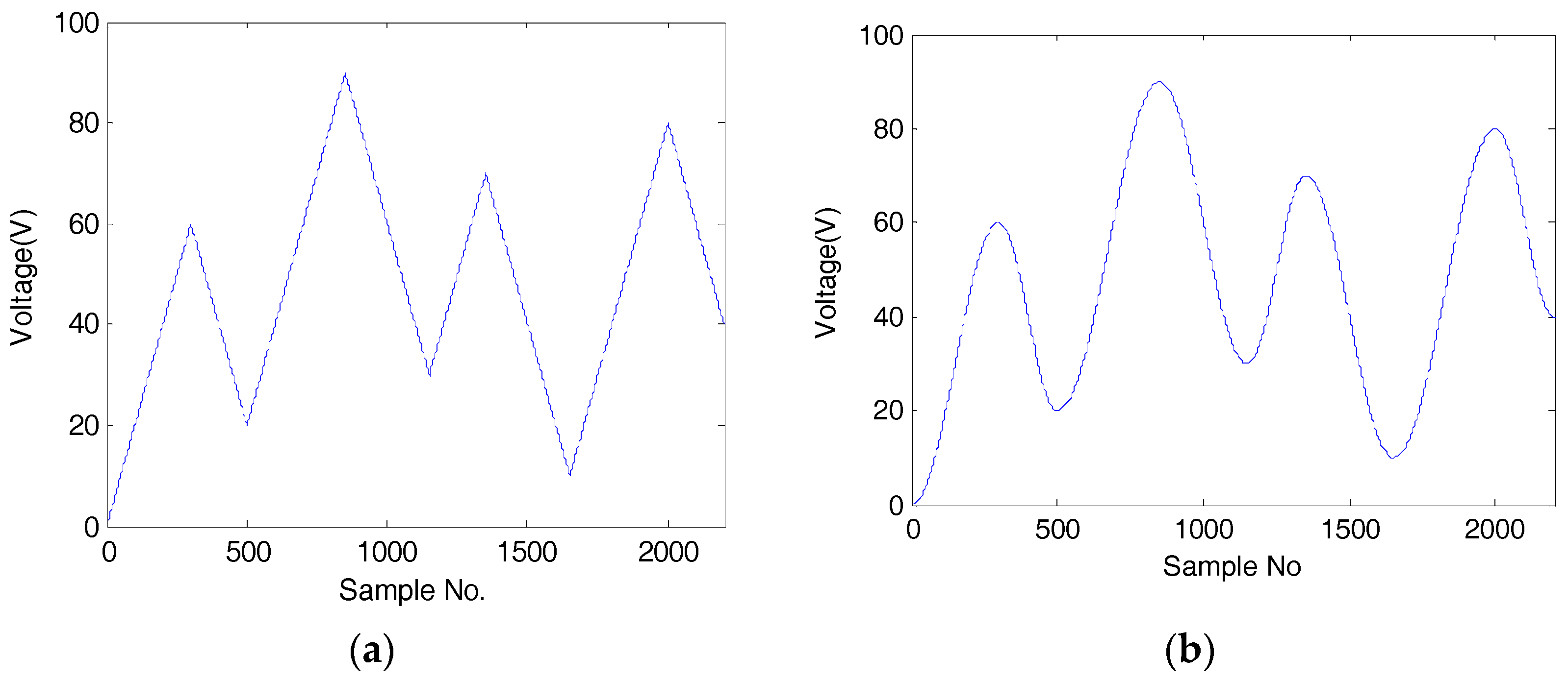
In this section, some experiments with two kinds of input waveforms (
Figure 17) at different rates are undertaken to prove the effectiveness of the proposed model. For comparison, the input excitations are also applied to the numerical Preisach model that is based on first reversal curves and is built according to Equation (26) [
9].
where
f(t) is the output displacement of the system;
v(t) is the input voltage.
is the elongation of the first reversal curve and
.
stands for the output of the first-order hysteresis curves when
.
is the output of the first-order hysteresis curves when the input
decrease to
from
c is the bias of the Preisach model. A triangle database of
with a grid resolution of 5 V and arange of
is obtained to prepare for the experiment in this work.
Figure 17.
The input excitations. (a) Triangular signals; (b) sinusoidal signals.
Figure 17.
The input excitations. (a) Triangular signals; (b) sinusoidal signals.
When implementing the proposed model, only the reference voltage sequence and the reference displacement sequence first need to be stored. While using the Preisach model, a limiting triangle database of the first-order reversal curve elongation, which is difficult to realize and record, needs to be stored in advance through experiments. Storing the database of the reference sequences is much easier than the one for first-order reversal curve elongation. When implementing the proposed model, the current displacement is obtained by only calculating several polynomials, which disclose the rules of hysteresis trajectories and take less computation time. However, the displacement in the Preisach model is obtained by calculating the summation of the weighted effective areas in the limiting triangle database, which is much more complex [
18].
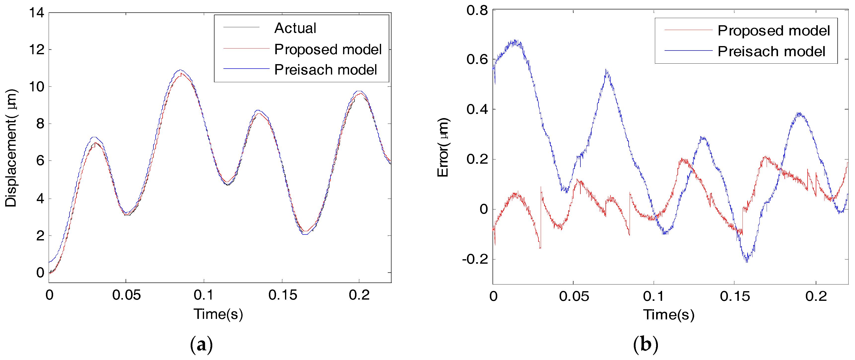
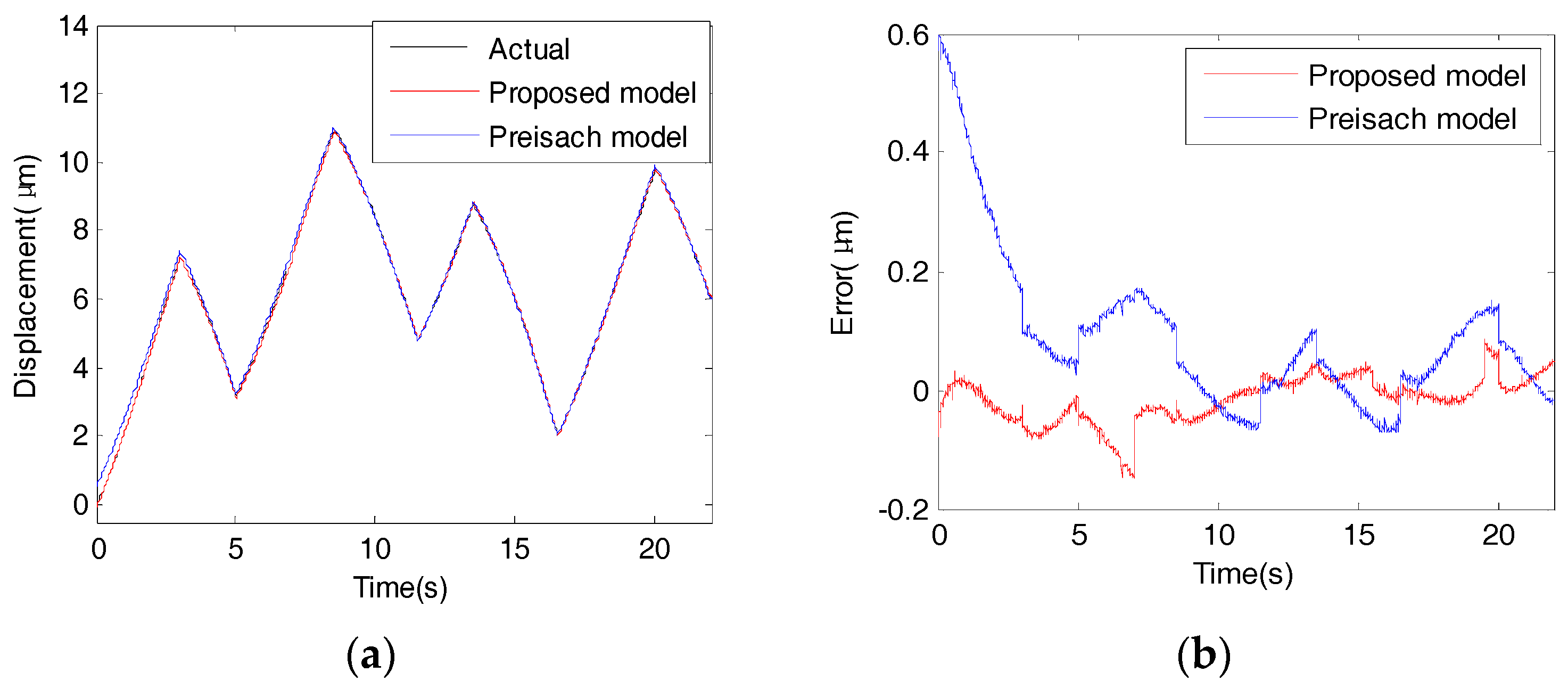
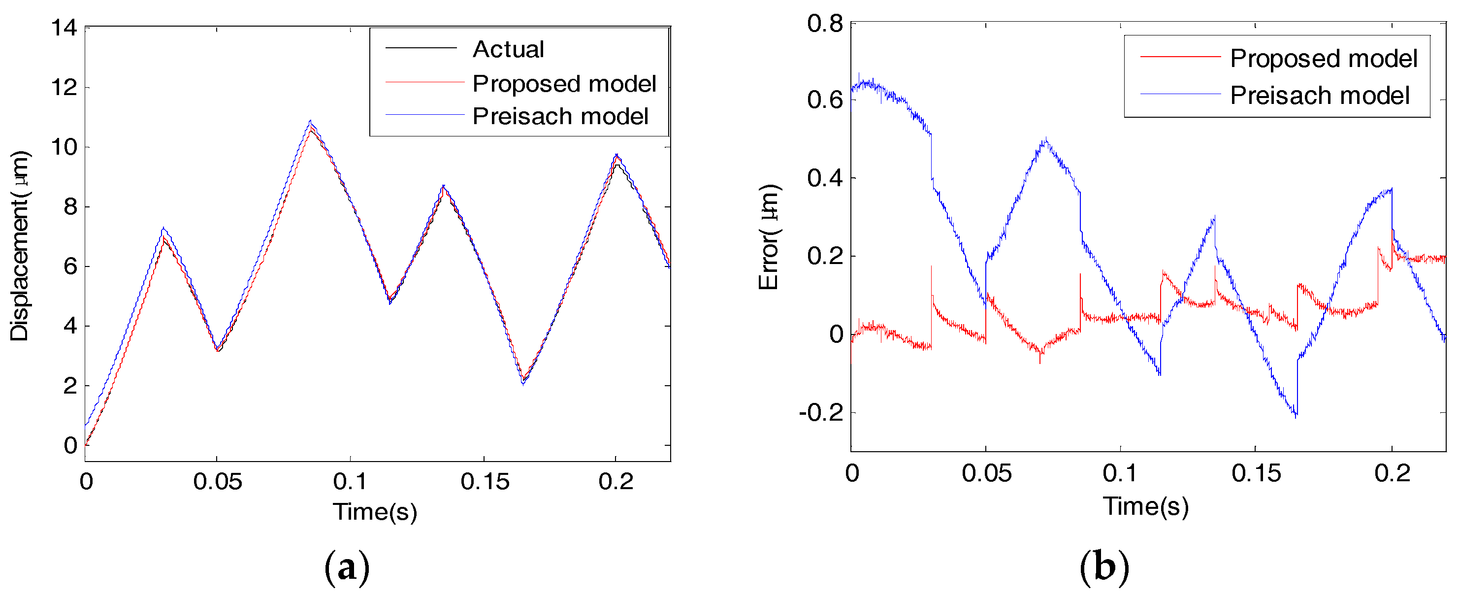
Figure 18 and
Figure 19 show the modeling performances of the proposed model and the Preisach model under the triangular input excitation (
Figure 17a) at low rate and high rate, respectively.
Table 7 gives the specific data of mean absolute errors (MAE) and root mean square error (RMSE). It is observed that when triangular input excitation with a low rate (20 V/s) is applied, the proposed model produces a MAE of 0.0319 μm and a RMSE of 0.0421 μm, which accounts for 0.2924% and 0.3851% of the motion range, respectively. While using the Preisach model, the corresponding MAE and RMSE are 0.1067 μm and 0.1627 μm, which account for 0.9780% and 1.4913% respectively. In the case of high rate (2000 V/s), using the proposed model, the MAE and MSE are 0.0644 μm and 0.0854 μm, which are equivalent to 0.6153% and 0.8159% of the overall motion range, respectively. The Preisach model produces a MAE of 0.2475 μm and a RMSE of 0.3108 μm,
i.e., 2.3646% and 2.9694% of the overall motion range. The experimental results show that the proposed modeling method achieves high accuracy.
Table 7.
The modeling errors with sinusoidal excitations.
Table 7.
The modeling errors with sinusoidal excitations.
| Input Signal | Model | MAE (μm) | RMSE (μm) |
|---|
| Low rate | Triangular | Proposed model | 0.0319 | 0.0421 |
| Preisach model | 0.1067 | 0.1627 |
| sinusoidal | Proposed model | 0.0523 | 0.0615 |
| Preisach model | 0.1352 | 0.1896 |
| High rate | Triangular | Proposed model | 0.0644 | 0.0854 |
| Preisach model | 0.2475 | 0.3108 |
| sinusoidal | Proposed model | 0.0727 | 0.0911 |
| Preisach model | 0.2445 | 0.3087 |
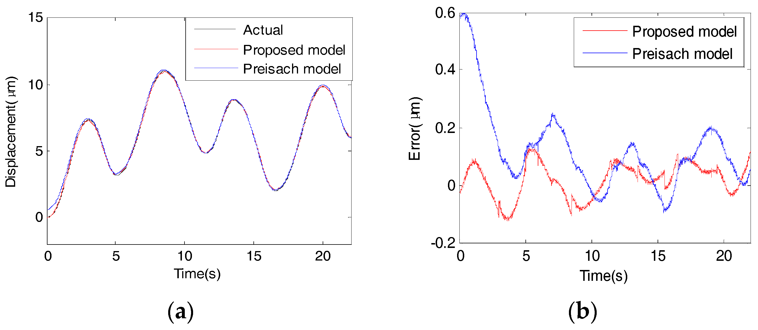
Figure 20 and
Figure 21 show the modeling performances of the proposed model and the Preisach model under the sinusoidal input excitation (
Figure 17b) at low rate and high rate, respectively.
Table 7 gives the specific data of MAE and RMSE. When applying sinusoidal input excitation with low rate, the proposed model produce a MAE of 0.0532 μm and a RMSE of 0.0615 μm,
i.e., 0.4716% and 0.5546% of the motion range, respectively. While using the Preisach model, the MAE and RMSE are 0.1352 μm and 0.1896 μm,
i.e., 1.2191% and 1.171% of the overall motion range, respectively. When applying sinusoidal signals with a high rate, the MAE and MSE of the proposed model are 0.0727 μm and 0.0911 μm,
i.e., 0.6946% and 0.8704% of the overall motion range, respectively. The Preisach model produces a MAE of 0.2445 μm and a RMSE of 0.3087 μm,
i.e., 2.3360% and 2.9494% of the motion range.
Figure 18.
The responses triangular excitation with a low rate. (a) The output displacement curves; (b) error curves.
Figure 18.
The responses triangular excitation with a low rate. (a) The output displacement curves; (b) error curves.
Figure 19.
The responses to the random triangular excitation with high rate. (a) The output displacement curves; (b) error curves.
Figure 19.
The responses to the random triangular excitation with high rate. (a) The output displacement curves; (b) error curves.
Figure 20.
The responses to sinusoidal excitation with a low rate. (a) The output displacement curves; (b) error curves.
Figure 20.
The responses to sinusoidal excitation with a low rate. (a) The output displacement curves; (b) error curves.
Figure 21.
The responses to sinusoidal excitation with high rate. (a) Output displacement curves; (b) error curves.
Figure 21.
The responses to sinusoidal excitation with high rate. (a) Output displacement curves; (b) error curves.
From the experimental results, it is observed that although the similarity relationships are obtained by using the triangular input voltage excitation, the model is also effective when giving other input waveforms. This proposed model can achieve good performance at both low rate and high rate. The modeling ability of the proposed model is better than that of the Preisach model.
7. Conclusions
In this paper, a novel modeling method using segment-similarity of hysteresis nonlinearity in a piezoelectric actuator is proposed. First, the segment-similarity of the hysteresis curves has been presented by using triangular input excitations with different extremes. Segment similarity describes the similarity relationship between hysteresis curve segments with the same voltage interval that depart from different turning points. However, the similarity is only suitable for the hysteresis curve segments that have turning points on the reference curve. For others, large errors may be produced. Therefore, based on the inherent hysteresis properties of a PZA, a modified segment-similarity relationship is proposed to disclose how the coordinates of turning points determine the hysteresis curve. Time-scale similarity is used to obtain a dynamic model. It is remarked that the proposed model is easily established and is more straightforward and simpler and takes less computation time than the Preisach model.
Experiments with different input excitations were carried out. The experimental results demonstrate that the proposed model has good performance in hysteresis trajectory prediction and performs better than the Preisach model. Moreover, although the similarity relationship is concluded from the triangular sequences, the proposed model is suitable for other waveforms. It is expected that the proposed method can be also effectively applied in accurate hysteresis prediction for other smart materials that have similar properties. In future work, the proposed model-based hysteresis compensator will be designed to reduce or eliminate the hysteresis effect in high-precision control systems.


