
A Two-Dimensional Precision Level for Real-Time Measurement Based on Zoom Fast Fourier Transform

 ,
,  ,
,  ,
,  ,
, 
Abstract
:1. Introduction
2. Principles and Methods
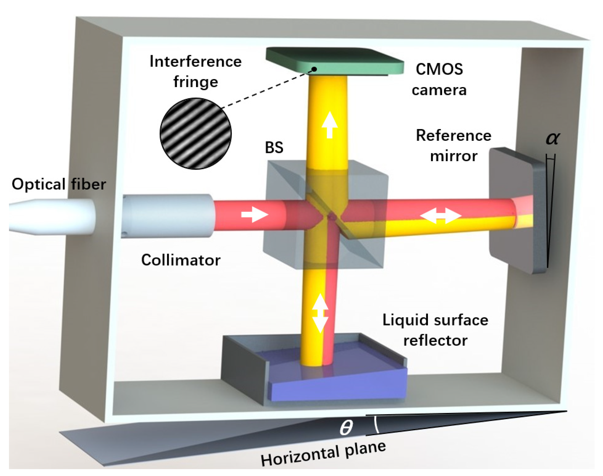
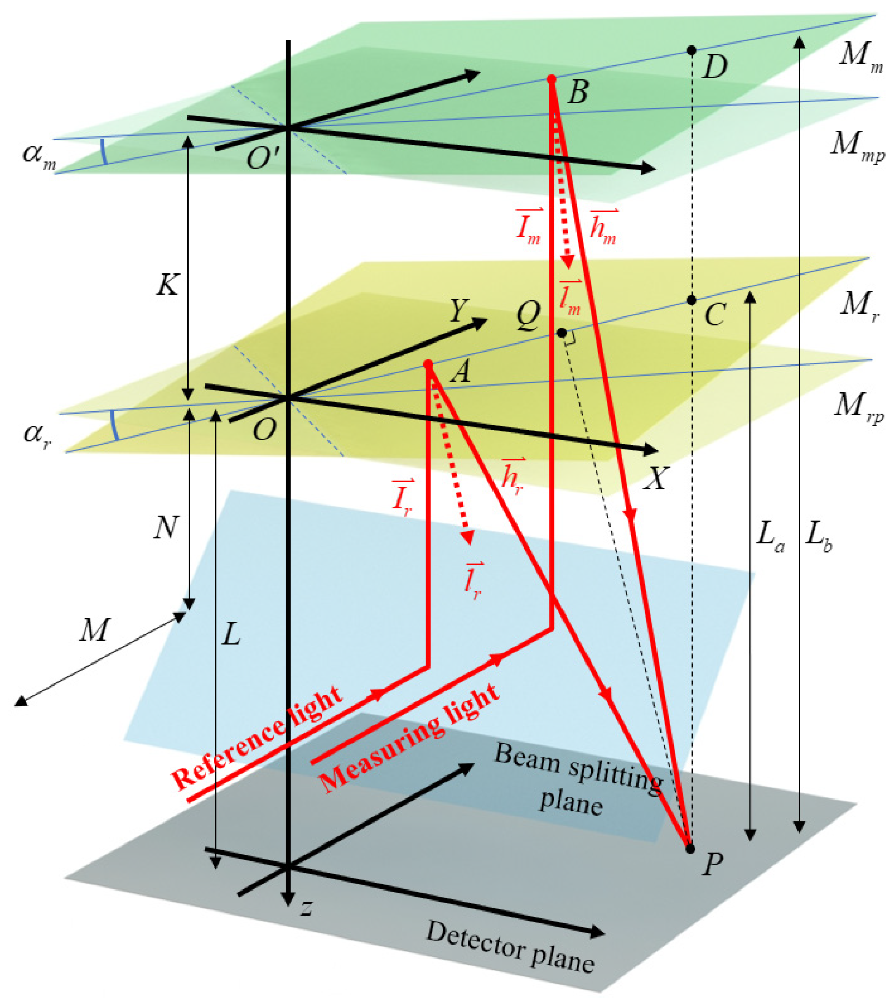
2.1. Structure and Angle Measurement Method of Level
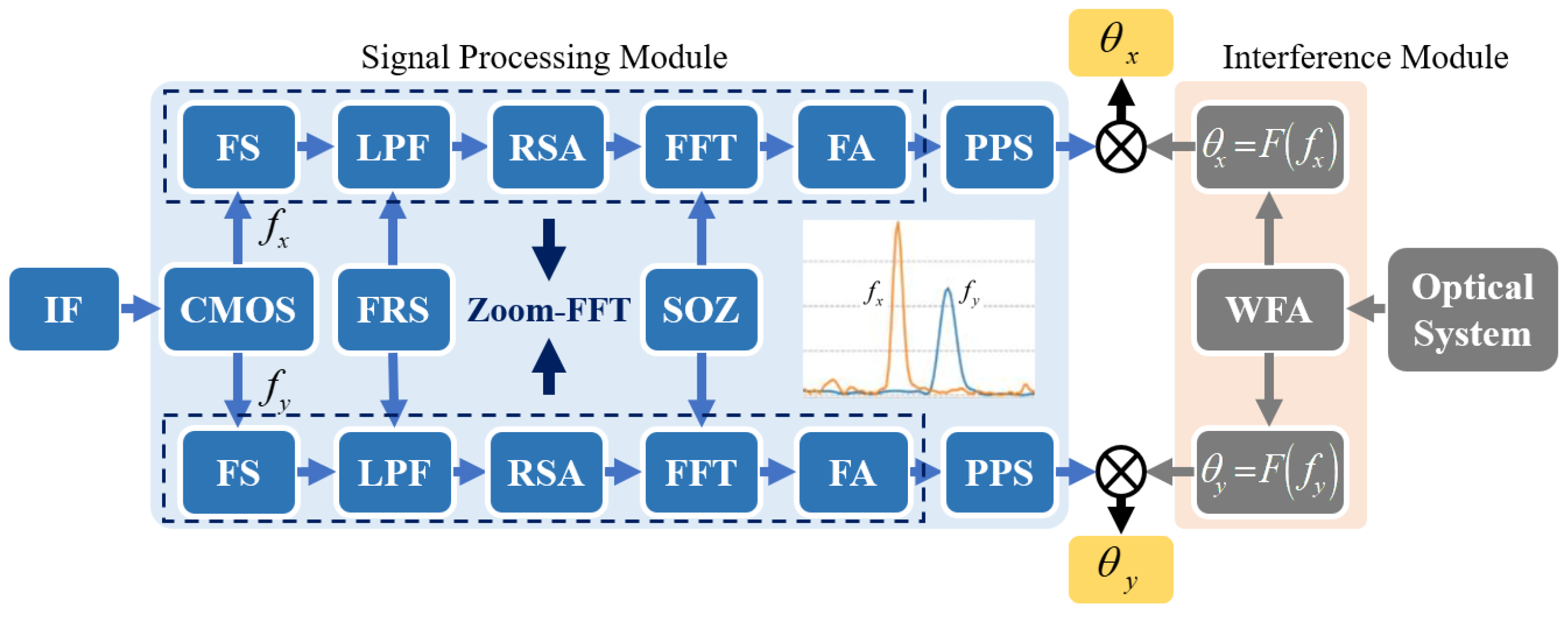
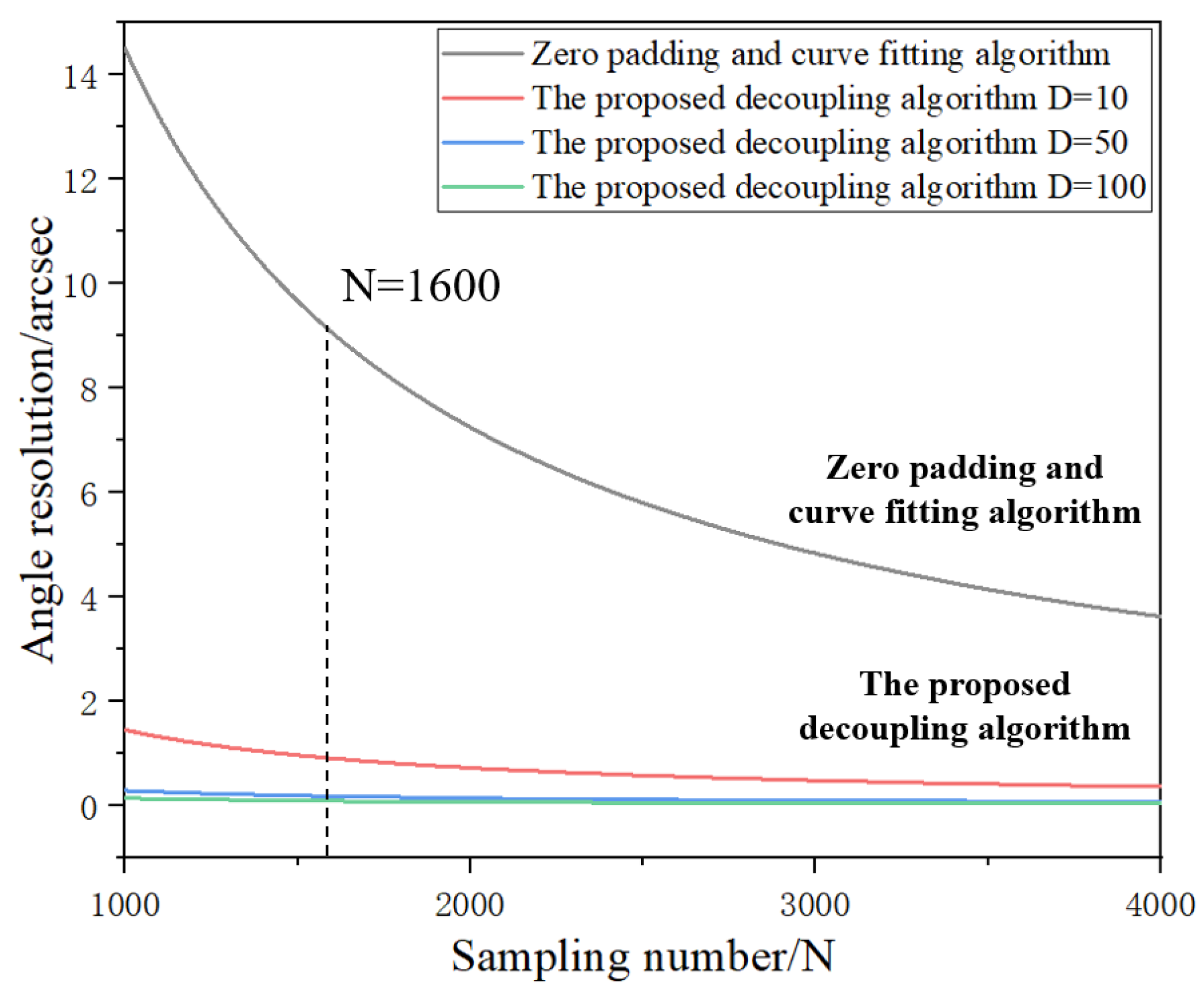
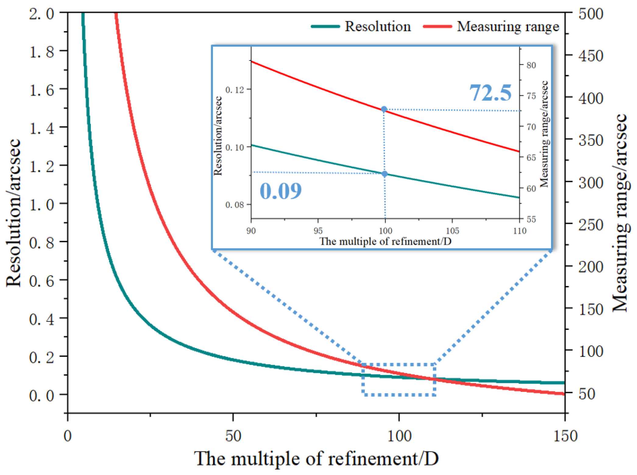
2.2. High-Resolution-Angle-Decoupling Algorithm Based on Zoom FFT
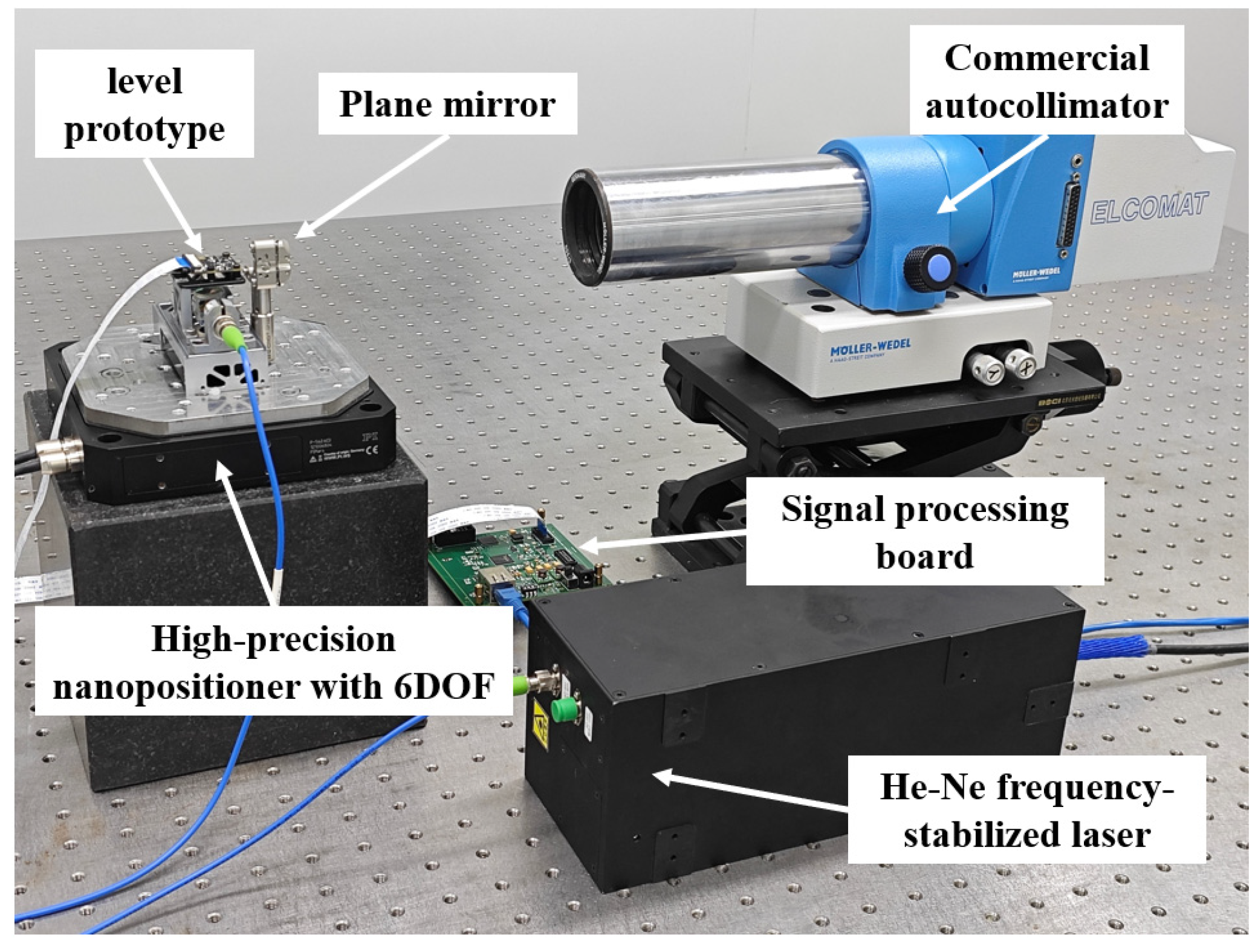
3. Experimental Results
3.1. Functional Verification of Signal Processing Board
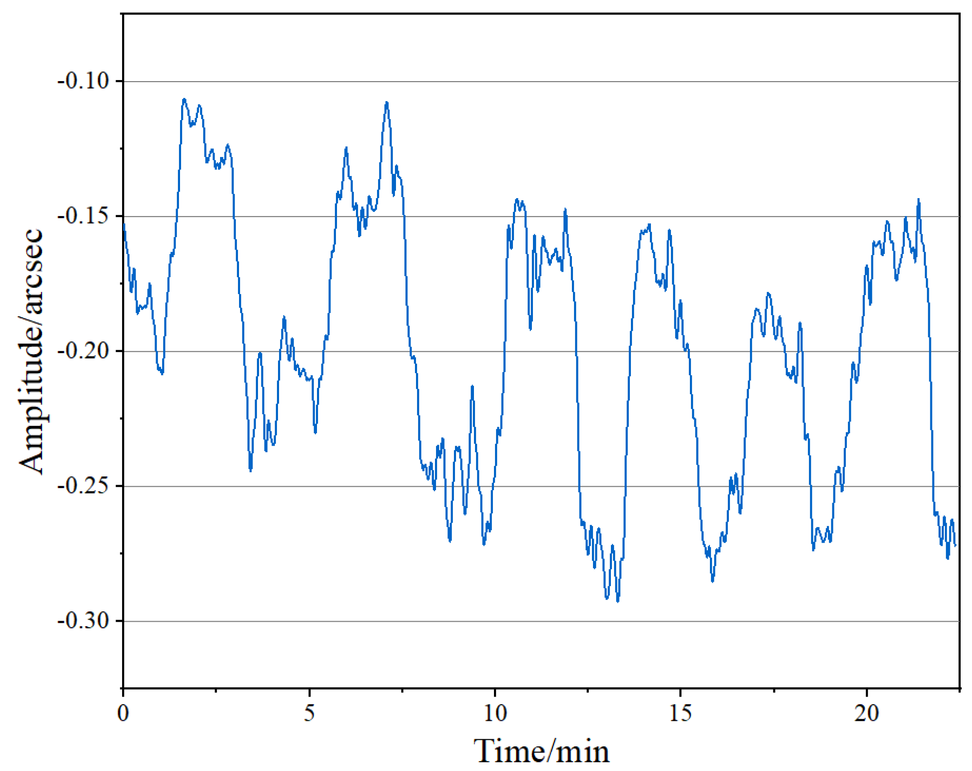
3.2. Stability Test of the Proposed Level
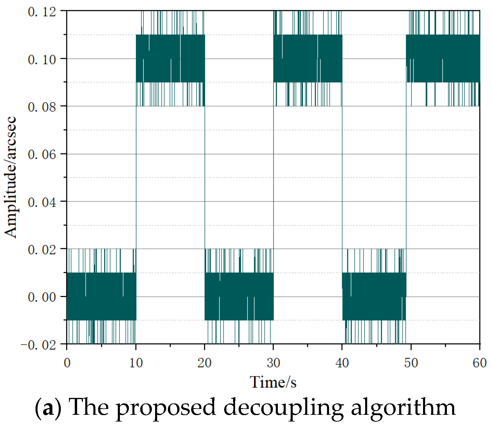
3.3. Repeatability Test of the Proposed Level
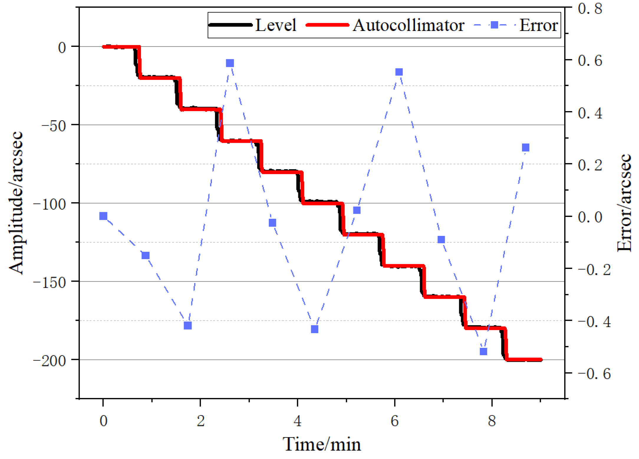
3.4. Angle Measurement Accuracy Test of the Proposed Level
4. Conclusions
Author Contributions
Funding
Data Availability Statement
Conflicts of Interest
References
- Peng, W.; Xia, H.; Wang, S.; Chen, X. Measurement and identification of geometric errors of translational axis based on sensitivity analysis for ultra-precision machine tools. Int. J. Adv. Manuf. Technol. 2018, 94, 2905–2917. [Google Scholar] [CrossRef]
- Shimizu, Y.; Kataoka, S.; Ishikawa, T.; Chen, Y.L.; Chen, X.; Matsukuma, H.; Gao, W. A Liquid-Surface-Based Three-Axis Inclination Sensor for Measurement of Stage Tilt Motions. Sensors 2018, 18, 398. [Google Scholar] [CrossRef] [PubMed]
- Yu, L.; Molnar, G.; Werner, C.; Weichert, C.; Köning, R.; Danzebrink, H.U.; Tan, J.; Flügge, J. A Single-beam 3DoF Homodyne Interferometer. Meas. Sci. Technol. 2020, 31, 084006. [Google Scholar] [CrossRef]
- Zhang, C.; Duan, F.; Fu, X.; Liu, C.; Liu, W.; Su, Y. Dual-axis optoelectronic level based on laser auto-collimation and liquid surface reflection. Opt. Laser Technol. 2019, 113, 357–364. [Google Scholar] [CrossRef]
- Fan, K.; Wang, T.; Lin, S.; Liu, Y. Design of a dual-axis optoelectronic level for precision angle measurements. Meas. Sci. Technol. 2011, 22, 055302. [Google Scholar] [CrossRef]
- Zeng, T.; Lu, Y.; Liu, Y.; Yang, H.; Bai, Y.; Hu, P.; Li, Z.; Zhang, Z.; Tan, J. A Capacitive Sensor for the Measurement of Departure From the Vertical Movement. IEEE Trans. Instrum. Meas. 2016, 65, 458–466. [Google Scholar] [CrossRef]
- Zeng, T.; Lu, Y.; Chen, L.; Fu, Y.; Xu, S. 2-D Vertical Filament Capacitive Sensor for the Measurement in Vacuum Environment. IEEE Trans. Instrum. Meas. 2018, 67, 2382–2389. [Google Scholar] [CrossRef]
- Perchat, R.; Mccarty, R. Multi-axis Bubble Vial Device. US Patent 7497021, 26 July 2007. [Google Scholar]
- Brook Automation Co. High Resolution Electronic Level Wafer EL-3003 User Manual. Available online: http://www.datasheets.com/en/part-details/el-3003-brooks-automation-98521329 (accessed on 15 August 2023).
- Antunes, P.; Marques, C.; Varum, H.; Andre, P. Biaxial optical accelerometer and high-angle inclinometer with temperature and cross-axis insensitivity. IEEE Sens. J. 2012, 12, 2399–2406. [Google Scholar] [CrossRef]
- Moura, J.; Silva, S.; Becker, M.; Rothardt, M.; Bartelt, H.; Santos, J.; Frazal, O. Optical inclinometer based on a phase-shifted Bragg grating in a taper configuration. IEEE Photon. Technol. Lett. 2014, 26, 405–407. [Google Scholar] [CrossRef]
- Li, C.; Li, X.; Yu, X.; Peng, X.; Lan, T.; Fan, S. Room-Temperature Wide Measurement Range Optical Fiber Fabry-Perot Tilt Sensor with Liquid Marble. IEEE Sens. J. 2018, 18, 170–177. [Google Scholar] [CrossRef]
- Wang, S.; Yang, Y.; Mohanty, L.; Jin, R.; Lu, P. Ultrasensitive Fiber Optic Inclinometer Based on Dynamic Vernier Effect Using Push Pull Configuration. IEEE Trans. Instrum. Meas. 2022, 71, 7006408. [Google Scholar] [CrossRef]
- Huang, Y.; Fan, Y.; Lou, Z.; Fan, K.; Sun, W. An Innovative Dual-Axis Precision Level Based on Light Transmission and Refraction for Angle Measurement. Appl. Sci. 2020, 10, 6019. [Google Scholar] [CrossRef]
- Torng, J.; Wang, C.; Huang, Z.; Fan, K. A novel dual-axis optoelectronic level with refraction principle. Meas. Sci. Technol. 2013, 24, 035902. [Google Scholar] [CrossRef]
- Li, R.; Ma, S.; Xu, P.; Pan, Q.; Wei, Y.; Fan, K. Development of a high-sensitivity dual axis optoelectronic level using double-layer liquid refraction. Opt. Laser Eng. 2021, 146, 106696. [Google Scholar] [CrossRef]
- Zeng, T.; Lu, Y.; Yang, H.; Hu, P.; Liu, Y.; Li, Z.; Zhang, Z. System for the measurement of the deviation of a laser beam from the vertical direction. Appl. Opt. 2016, 55, 2692–2700. [Google Scholar] [CrossRef] [PubMed]
- Hu, P.; Lin, X.; Zhang, Y.; Yu, L. A Dual-Axis Optoelectronic Inclinometer Based on Wavefront Interference Fringes. IEEE Trans. Instrum. Meas. 2023, 72, 3272378. [Google Scholar] [CrossRef]
- Molnar, G.; Strube, S.; Kochert, P.; Danzebrink, H.; Flügge, J. Simultaneous multiple degrees of freedom (DOF) measurement system. Meas. Sci. Technol. 2016, 27, 084011. [Google Scholar] [CrossRef]
- Strube, S.; Molnar, G.; Danzebrink, H. Compact field programmable gate array (FPGA)-based multi-axial interferometer for simultaneous tilt and distance measurement in the sub-nanometre range. Meas. Sci. Technol. 2011, 22, 094026. [Google Scholar] [CrossRef]
- Yu, L.; Molnar, G.; Butefisch, S.; Werner, C.; Meeß, R.; Danzebrink, H.; Flügge, J. Micro Coordinate Measurement Machine (uCMM) using voice coil actuator with interferometric position feedback. Proc. Spie 2019, 11053, 463–468. [Google Scholar]
- De Zanet, G.; Viquerat, A.; Aglietti, G. Dynamic interferometric measurements of thermally-induced deformations on telescope based on high-strain composite tape-springs. Thin-Walled Struct. 2022, 179, 109657. [Google Scholar] [CrossRef]
- Lou, Y.; Yan, L.; Chen, B.; Zhang, S. Laser homodyne straightness interferometer with simultaneous measurement of six degrees of freedom motion errors for precision linear stage metrology. Opt. Express 2017, 25, 6805–6821. [Google Scholar] [CrossRef] [PubMed]


Disclaimer/Publisher’s Note: The statements, opinions and data contained in all publications are solely those of the individual author(s) and contributor(s) and not of MDPI and/or the editor(s). MDPI and/or the editor(s) disclaim responsibility for any injury to people or property resulting from any ideas, methods, instructions or products referred to in the content. |
© 2023 by the authors. Licensee MDPI, Basel, Switzerland. This article is an open access article distributed under the terms and conditions of the Creative Commons Attribution (CC BY) license (https://creativecommons.org/licenses/by/4.0/).
Share and Cite
Fu, H.; Wang, Z.; Lin, X.; Xing, X.; Yang, R.; Yang, H.; Hu, P.; Ding, X.; Yu, L. A Two-Dimensional Precision Level for Real-Time Measurement Based on Zoom Fast Fourier Transform. Micromachines 2023, 14, 2028. https://doi.org/10.3390/mi14112028
Fu H, Wang Z, Lin X, Xing X, Yang R, Yang H, Hu P, Ding X, Yu L. A Two-Dimensional Precision Level for Real-Time Measurement Based on Zoom Fast Fourier Transform. Micromachines. 2023; 14(11):2028. https://doi.org/10.3390/mi14112028
Chicago/Turabian StyleFu, Haijin, Zheng Wang, Xionglei Lin, Xu Xing, Ruitao Yang, Hongxing Yang, Pengcheng Hu, Xuemei Ding, and Liang Yu. 2023. "A Two-Dimensional Precision Level for Real-Time Measurement Based on Zoom Fast Fourier Transform" Micromachines 14, no. 11: 2028. https://doi.org/10.3390/mi14112028
APA StyleFu, H., Wang, Z., Lin, X., Xing, X., Yang, R., Yang, H., Hu, P., Ding, X., & Yu, L. (2023). A Two-Dimensional Precision Level for Real-Time Measurement Based on Zoom Fast Fourier Transform. Micromachines, 14(11), 2028. https://doi.org/10.3390/mi14112028