
Numerical and Experimental Validation of Mixing Efficiency in Periodic Disturbance Mixers

 ,
,  ,
,  , and
, and
Abstract
: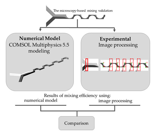
1. Introduction
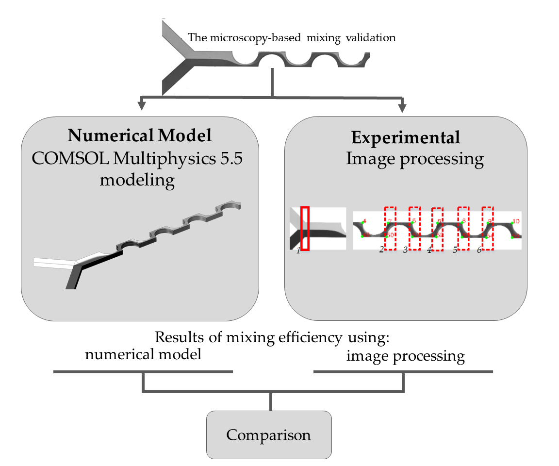
2. Materials and Methods
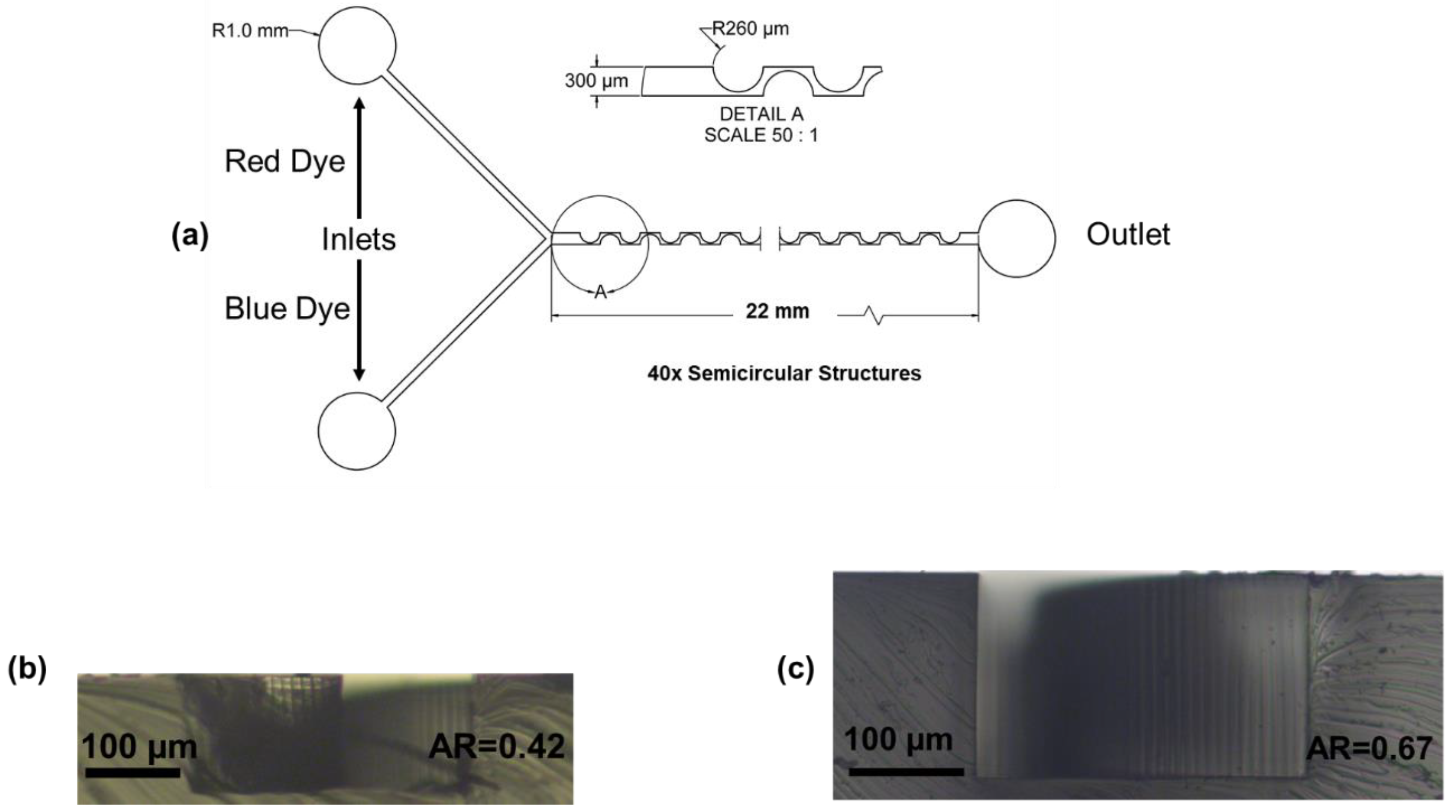
2.1. Periodic Disturbance Mixer Design and Fabrication
2.2. Numerical Modeling of Micromixing
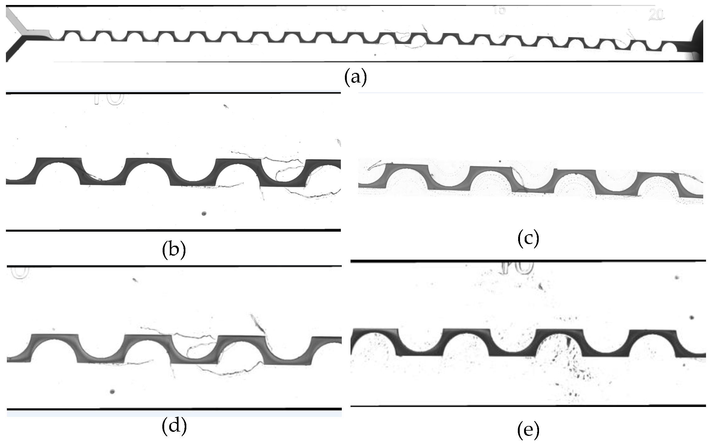
2.3. Mixing Imaging
2.3.1. Image Dataset of the Experimental Results
2.3.2. Extraction and Evaluation of Characteristics
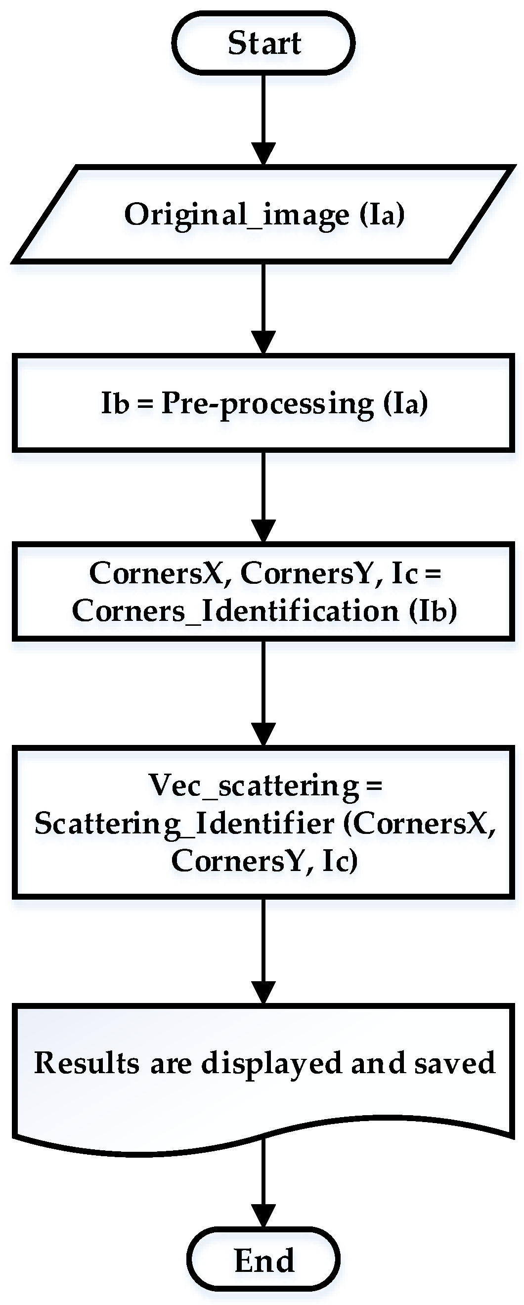
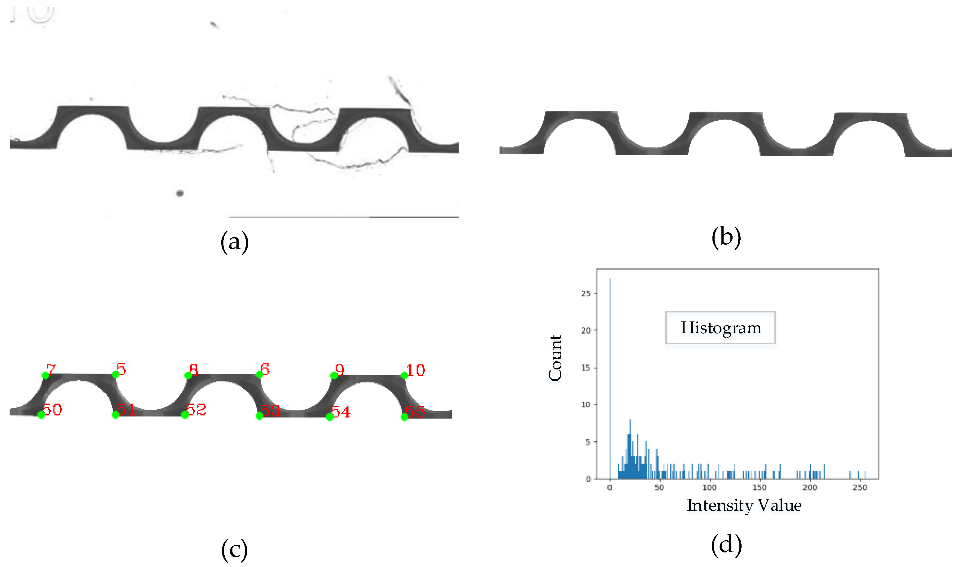
2.3.3. Pre-Processing Stage
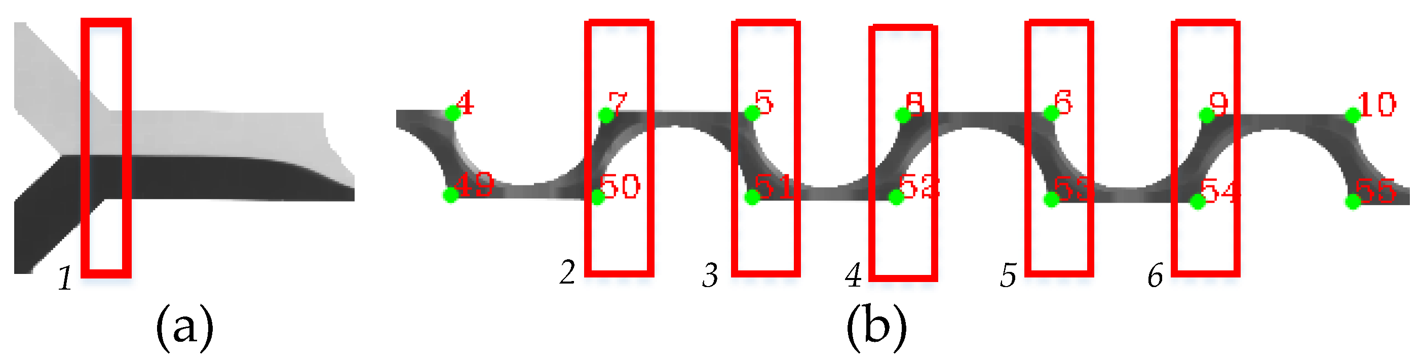
2.3.4. Identification of Corners and Evaluation of Gray Intensity
2.3.5. Calculation of Mixing Efficiency
2.3.6. Training and Validation
3. Results and Discussion
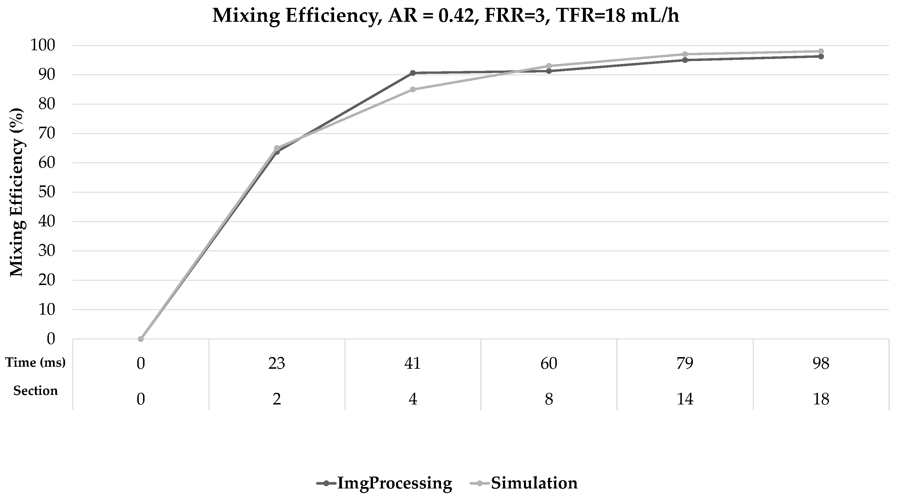
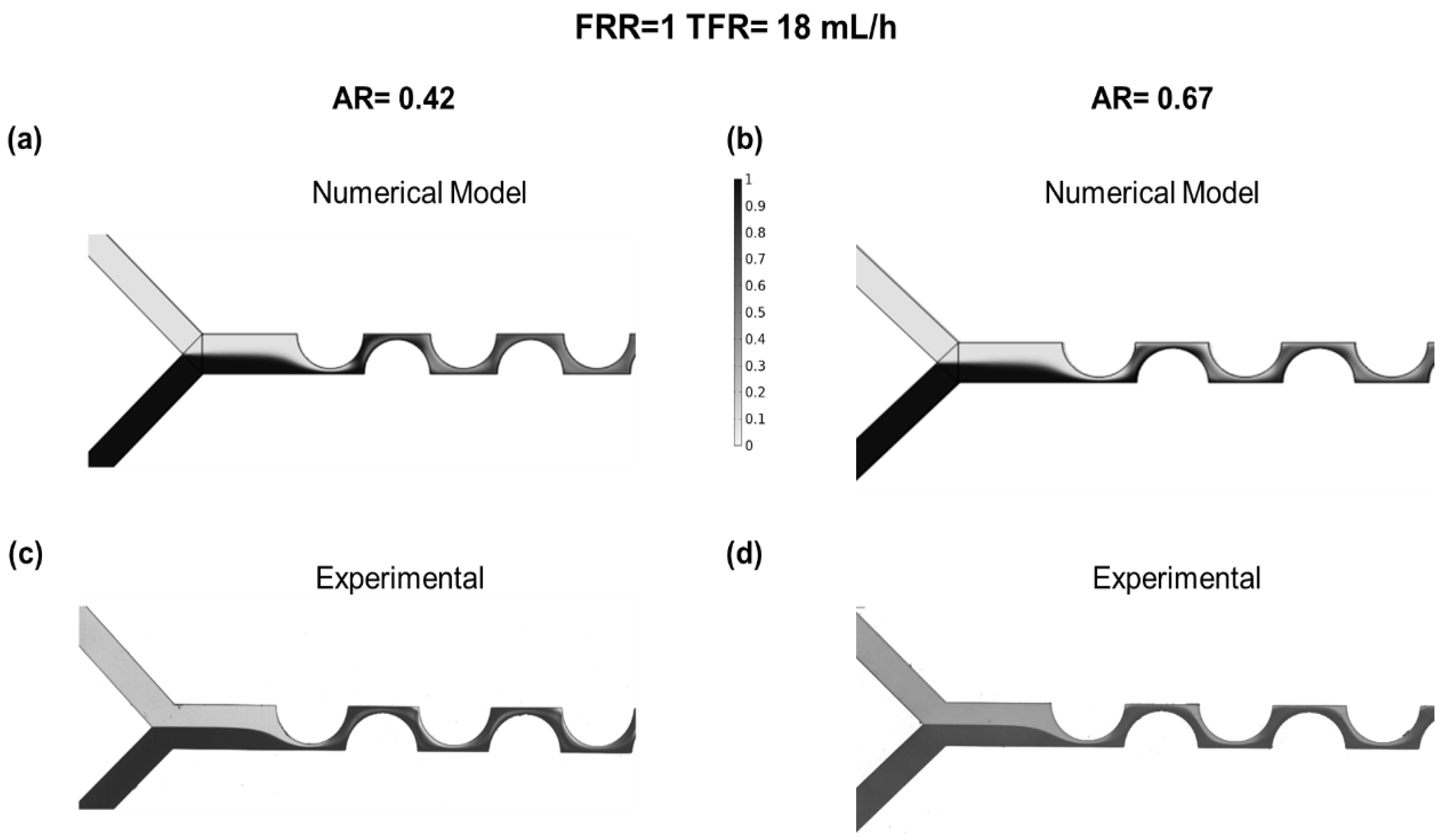
3.1. PDM Mixing at Different AR Numerical Modeling and Experimental Results
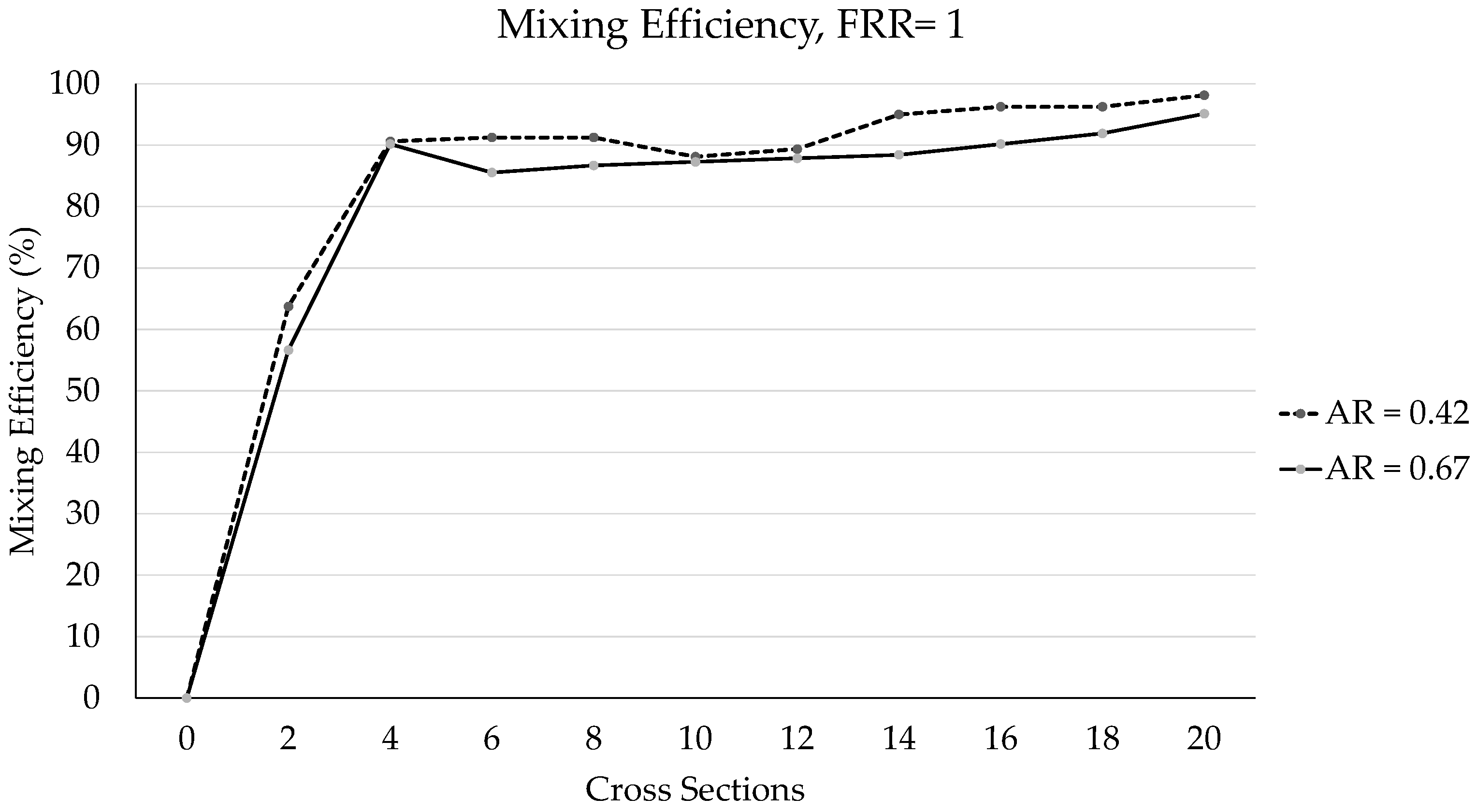
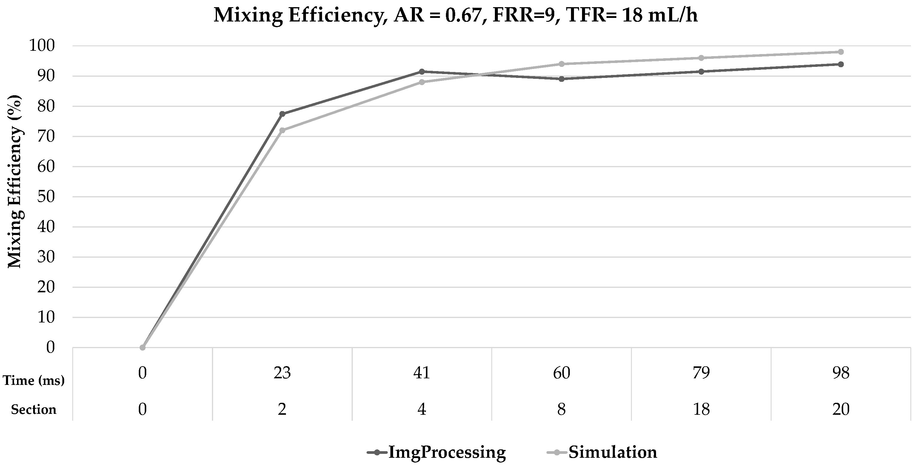
3.2. PDM Mixing Efficiency Performance at the Cross-Sections
4. Conclusions
Supplementary Materials
Author Contributions
Funding
Data Availability Statement
Acknowledgments
Conflicts of Interest
Appendix A
| Algorithm A1. Proposed method to remove noise, showing lines 1–9, corresponding to the images in Figure 3b. |
| Input: , input image. |
| Output: , denoised image, identified contour. |
| 1: procedure Pre-processing () |
| 2: |
| 3: |
| 4: |
| 5: ▹ scale is thickness |
| 6: |
| 7: |
| 8: ▹ K1, K2 are the kernel |
| 9: |
| Algorithm A2. Proposed method for identifying corners, showing lines 1–11, corresponding to the images in Figure 3d. |
| Input: , input image. |
| Output: , identified corners, CornersX, CornersY. |
| 1: procedure IntensityEvaluation() |
| 2: ▹ thickness of stripes in pixels |
| 3: |
| 4: |
| 5: |
| 6: for all i do |
| 7: |
| 8: |
| 9: |
| 10: |
| 11: |
References
- Gaozhe, C.; Li, X.; Huilin, Z.; Jianhan, L. A review on micromixers. Micromachines 2017, 8, 274. [Google Scholar]
- An, N.; Deng, H.; Devendran, C.; Akhtar, N.; Ma, X.; Pouton, C.; Chan, H.; Neild, A.; Alan, T. Ultrafast star-shaped acoustic micromixer for high throughput nanoparticle synthesis. Lab Chip 2020, 20, 582–591. [Google Scholar] [CrossRef]
- Maeki, M.; Fujishima, Y.; Sato, Y.; Yasui, T.; Kaji, N.; Ishida, A.; Tani, H.; Baba, Y.; Harashima, H.; Tokeshi, M. Understanding the formation mechanism of lipid nanoparticles in microfluidic devices with chaotic micromixers. PLoS ONE 2017, 12, e0187962. [Google Scholar] [CrossRef]
- Ansari, M.; Kim, K.; Anwar, K.; Kim, S. A novel passive micromixer based on unbalanced splits and collisions of fluid streams. J. Micromech. Microeng. 2010, 20, 055007. [Google Scholar] [CrossRef] [Green Version]
- Jahn, A.; Vreeland, W.; DeVoe, D.; Locascio, L.; Gaitan, M. Microfluidic Directed Formation of Liposomes of Controlled Size. Langmuir 2007, 6289–6293. [Google Scholar] [CrossRef]
- Nguyen, N. Chapter 1—Introduction. In Micromixers, 2nd ed.; William Andrew Publishing: Oxford, UK, 2012; pp. 1–8. [Google Scholar]
- Javaid, M.; Cheema, T.; Park, C. Analysis of Passive Mixing in a Serpentine Microchannel with Sinusoidal Side Walls. Micromachines 2018, 28, 8. [Google Scholar] [CrossRef] [Green Version]
- Jen, C.-P.; Wu, C.-Y.; Lin, Y.-C.; Wu, C.-Y. Design and simulation of the micromixer with chaotic advection in twisted microchannels. Lab Chip 2003, 77–81. [Google Scholar] [CrossRef] [PubMed]
- Nguyen, N.; Wu, Z. Micromixers a review. J. Micromechan. Microeng. 2005, 15, R1–R16. [Google Scholar] [CrossRef]
- Nguyen, N. Chapter 7—Active micromixers. In Micromixers, 2nd ed.; William Andrew Publishing: Oxford, UK, 2012; pp. 239–294. [Google Scholar]
- Oddy, M.; Santiago, J.; Mikkelsen, J. Electrokinetic Instability Micromixing. Anal. Chem. 2001, 5822–5832. [Google Scholar] [CrossRef]
- Wu, Y.; Ren, Y.; Tao, Y.; Hou, L.; Hu, Q.; Jiang, H. A novel micromixer based on the alternating current-flow field effect transistor. Lab Chip 2016, 186–197. [Google Scholar] [CrossRef]
- Yang, F.; Kuang, C.; Zhao, W.; Wang, G. Electrokinetic Fast Mixing in Non-Parallel Microchannels. Chem. Eng. Commun. 2017, 204, 190–197. [Google Scholar] [CrossRef]
- Capretto, L.; Cheng, W.; Hill, M.; Zhang, X. Micromixing Within Microfluidic Devices. Top. Curr. Chem. 2011, 304, 27–68. [Google Scholar] [CrossRef] [PubMed]
- Lee, C.; Chang, C.; Wang, Y.; Fu, L. Microfluidic Mixing: A Review. Int. J. Mol. Sci. 2011, 12, 3263–3287. [Google Scholar] [CrossRef] [PubMed] [Green Version]
- Johnson, J.; Ross, D.; Locascio, L. Rapid Microfluidic Mixing. Anal. Chem. 2002, 74, 45–51. [Google Scholar] [CrossRef]
- Cheung, C.C.L.; Al-Jamal, W.T. Sterically stabilized liposomes production using staggered herringbone micromixer: Effect of lipid composition and PEG-lipid content. Int. J. Pharm. 2019, 566, 687–696. [Google Scholar] [CrossRef]
- Ansari, A.; Kim, K.; Kim, S. Numerical and Experimental Study on Mixing Performances of Simple and Vortex Micro T-Mixers. Micromachines 2018, 9, 204. [Google Scholar] [CrossRef] [Green Version]
- Wong, S.; Ward, M.; Wharton, C. Micro T-mixer as a rapid mixing micromixer. Sens. Actuators B Chem. 2004, 100, 359–379. [Google Scholar] [CrossRef]
- Kastner, E.; Verma, V.; Lowry, D.; Perrie, Y. Microfluidic-controlled manufacture of liposomes for the solubilization of a poorly water-soluble drug. Int. J. Pharm. 2015, 485, 122–130. [Google Scholar] [CrossRef] [Green Version]
- Lim, T.; Son, Y.; Jeong, Y.; Yang, D.; Kong, H.; Lee, K.; Kim, D. Three-dimensionally crossing manifold micro-mixer for fast mixing in a short channel length. Lab Chip 2011, 11, 100–103. [Google Scholar] [CrossRef] [Green Version]
- Kimura, N.; Maeki, M.; Sato, Y.; Note, Y.; Ishida, A.; Tani, H.; Harashima, H.; Tokeshi, M. Development of the iLiNP Device: Fine Tuning the Lipid Nanoparticle Size within 10 nm for Drug Delivery. ACS Omega 2018, 3, 5044–5051. [Google Scholar] [CrossRef]
- López, R.; Ocampo, I.; Sánchez, L.M.; Alazzam, A.; Bergeron, K.; Camacho-León, S.; Mounier, C.; Stiharu, I.; Nerguizian, V. Surface Response Based Modeling of Liposome Characteristics in a Periodic Disturbance Mixer. Micromachines 2020, 11, 235. [Google Scholar] [CrossRef] [PubMed] [Green Version]
- Kouadri, A.; Douroum, E.; Lasbet, Y.; Naas, T.T.; Khelladi, S.; Makhlouf, M. Comparative study of mixing behaviors using non-Newtonian fluid flows in passive micromixers. Int. J. Mech. Sci. 2021, 201, 106472. [Google Scholar] [CrossRef]
- Luo, X.; Cheng, Y.; Zhang, W.; Li, K.; Wang, P.; Zhao, W. Mixing performance analysis of the novel passive micromixer designed by applying fuzzy grey relational analysis. Int. J. Heat Mass Transf. 2021, 178, 121638. [Google Scholar] [CrossRef]
- Mashaei, P.; Asiaei, S.; Hosseinalipour, S. Mixing efficiency enhancement by a modified curved micromixer: A numerical study. Chem. Eng. Process. Process Intensif. 2020, 154, 108006. [Google Scholar] [CrossRef]
- Lee, J.; Lee, M.; Jung, C.; Park, Y.; Song, C.; Choi, M.; Park, H.; Park, J. High-throughput nanoscale lipid vesicle synthesis in a semicircular contraction-expansion array microchannel. BioChip J. 2013, 7, 210–217. [Google Scholar] [CrossRef]
- Yanar, F.; Mosayyebi, A.; Nastruzzi, C.; Carugo, D.; Zhang, X. Continuous-Flow Production of Liposomes with a Millireactor under Varying Fluidic Conditions. Pharmaceutics 2020, 12, 1001. [Google Scholar] [CrossRef]
- Shi, H.; Zhao, Y.; Liu, Z. Numerical investigation of the secondary flow effect of lateral structure of micromixing channel on laminar flow. Sens. Actuators B Chem. 2020, 321, 128503. [Google Scholar] [CrossRef]
- Forbes, C.W.N.; Roces, C.; Anderluzzi, G.; Lou, G.; Abraham, S.; Ingalls, L.; Marshall, K.; Leaver, T.; Watts, J. Using microfluidics for scalable manufacturing of nanomedicines from bench to GMP: A case study using protein-loaded liposomes. Int. J. Pharm. 2020, 582, 119266. [Google Scholar] [CrossRef]
- Fan, L.; Liang, X.; Hong, Z.; Jiang, Z.; Liang, Z. Rapid microfluidic mixer utilizing sharp corner structures. Microfluidics Nanofluidics 2017, 21, 36. [Google Scholar] [CrossRef]
- Danckwerts, P. The definition and measurement of some characteristics of mixtures. Appl. Sci. Res. 1952, 3, 279–296. [Google Scholar] [CrossRef]
- Nguyen, N. Chapter 8—Characterization techniques. In Micromixers, 2nd ed.; William Andrew Publishing: Oxford, UK, 2012; pp. 295–320. [Google Scholar]
- López, R.; Rubinat, P.; Sánchez, L.M.; Tsering, T.; Alazzam, A.; Bergeron, K.F.; Mounier, C.; Burnier, J.; Stiharu, I.; Nerguizian, V. The effect of different organic solvents in liposome properties produced in a periodic disturbance mixer: Transcutol, a potential organic solvent replacement. Colloids Surf. B Biointerfaces 2020, 198, 111447. [Google Scholar] [CrossRef] [PubMed]
- COMSOL. How to Inspect Your Mesh in COMSOL Multiphysics; COMSOL: Burlington, MA, USA, 2017. [Google Scholar]
- Gonzalez, R. Digital Image Processing; Pearson: Upper Saddle River, NJ, USA, 2008. [Google Scholar]
- Gunasegaran, T.; Cheah, Y.N. Evolutionary cross validation. In Proceedings of the IEEE 2017 8th International Conference on Information Technology (ICIT), Amman, Jordan, 17–18 May 2017; pp. 89–95. [Google Scholar] [CrossRef]
- Wong, K.W.; Fung, C.C.; Eren, H. A study of the use of self-organising map for splitting training and validation sets for backpropagation neural network. Proc. Digit. Process. Appl. 1996, 1, 157–162. [Google Scholar] [CrossRef]
- López, R.R.; Ocampo, I.; Font de Rubinat, P.G.; Sánchez, L.M.; Alazzam, A.; Tsering, T.; Bergeron, K.F.; Camacho-Léon, S.; Burnier, J.V.; Mounier, C.; et al. Parametric Study of the Factors Influencing Liposome Physicochemical Characteristics in a Periodic Disturbance Mixer. Langmuir 2021, 37, 8544–8556. [Google Scholar] [CrossRef] [PubMed]
- Nguyen, N.T. Chapter 2—Fundamentals of mass transport in the microscale. In Micromixers, 2nd ed.; William Andrew Publishing: Oxford, UK, 2012; pp. 9–72. [Google Scholar]


| Micromixer | Demonstrated Production Rate | Mixing Efficiency | Reference |
|---|---|---|---|
| Contraction Expansion Array (CEA) | 24 mL/h | 90% (120 ms whole channel) | [27] |
| iLiNP | 30 mL/h | 80–90% (<10 ms) | [22] |
| Periodic disturbance mixer (PDM) | 18 mL/h | 90% (approx. 95 ms) | [23] |
| MiliReactor | 600 mL/h | Not mentioned | [28] |
| Serpentine Micromixer | 9 mL/h | Not mentioned | [29] |
| Toroidal mixer design (TrM) | 20,000 mL/h | Not mentioned | [30] |
| Staggered Herringbone Micromixer | 60 mL/h | >80% | [17] |
| Mixer utilizing sharp corner structures | 12 mL/h | >35% | [31] |
| Parameter | Value | |||
|---|---|---|---|---|
| AR | 0.42 | 0.67 | ||
| Re | 68 | 19, 30, 41, 53, 64 | 47 | 13, 21, 28, 36, 44 |
| TFR (mL/h) | 18 | 5, 8, 11, 17 | 18 | 5, 8, 11, 17 |
| FRR | 1, 3, 5, 7, 9, 12 | 8.56 | 1, 3, 5, 7, 9, 12 | 8.56 |
| Property | Value |
|---|---|
| Mesh Vertices | 1,566,514 |
| Number of Elements | 5,685,617 |
| Minimum Element Quality | 0.01205 |
| Average Element Quality | 0.6294 |
| Element Volume Ratio | |
| Mesh volume m |
| Data | Time (ms) | 0 | 23 | 32 | 41 | 51 | 60 | 79 | Final |
|---|---|---|---|---|---|---|---|---|---|
| FRR = 1 | Gray intensity | 169 | 98 | 101 | 131 | 139 | 151 | 154 | 161 |
| % ME − Img Processing | 0% | 58% | 60% | 78% | 82% | 89% | 91% | 95% | |
| % ME − Numerical Model | 0% | 55% | 57% | 77% | 79% | 89% | 94% | 97% | |
| FRR = 3 | Gray intensity | 169 | 102 | 115 | 146 | 146 | 147 | 158 | 162 |
| % ME − Img Processing | 0% | 61% | 68% | 86% | 86% | 88% | 93% | 95% | |
| % ME − Numerical Model | 0% | 65% | 68% | 85% | 86% | 93% | 97% | 98% | |
| FRR = 9 | Gray intensity | 169 | 133 | 153 | 148 | 158 | 161 | 166 | 161 |
| % ME − Img Processing | 0% | 78% | 90% | 87% | 93% | 95% | 98% | 95% | |
| % ME − Numerical Model | 0% | 81% | 85% | 93% | 94% | 97% | 99% | 99% |
Publisher’s Note: MDPI stays neutral with regard to jurisdictional claims in published maps and institutional affiliations. |
© 2021 by the authors. Licensee MDPI, Basel, Switzerland. This article is an open access article distributed under the terms and conditions of the Creative Commons Attribution (CC BY) license (https://creativecommons.org/licenses/by/4.0/).
Share and Cite
López, R.R.; Sánchez, L.-M.; Alazzam, A.; Burnier, J.V.; Stiharu, I.; Nerguizian, V. Numerical and Experimental Validation of Mixing Efficiency in Periodic Disturbance Mixers. Micromachines 2021, 12, 1102. https://doi.org/10.3390/mi12091102
López RR, Sánchez L-M, Alazzam A, Burnier JV, Stiharu I, Nerguizian V. Numerical and Experimental Validation of Mixing Efficiency in Periodic Disturbance Mixers. Micromachines. 2021; 12(9):1102. https://doi.org/10.3390/mi12091102
Chicago/Turabian StyleLópez, Rubén R., Luz-María Sánchez, Anas Alazzam, Julia V. Burnier, Ion Stiharu, and Vahé Nerguizian. 2021. "Numerical and Experimental Validation of Mixing Efficiency in Periodic Disturbance Mixers" Micromachines 12, no. 9: 1102. https://doi.org/10.3390/mi12091102
APA StyleLópez, R. R., Sánchez, L.-M., Alazzam, A., Burnier, J. V., Stiharu, I., & Nerguizian, V. (2021). Numerical and Experimental Validation of Mixing Efficiency in Periodic Disturbance Mixers. Micromachines, 12(9), 1102. https://doi.org/10.3390/mi12091102