
Counterexample Generation for Probabilistic Model Checking Micro-Scale Cyber-Physical Systems


Abstract
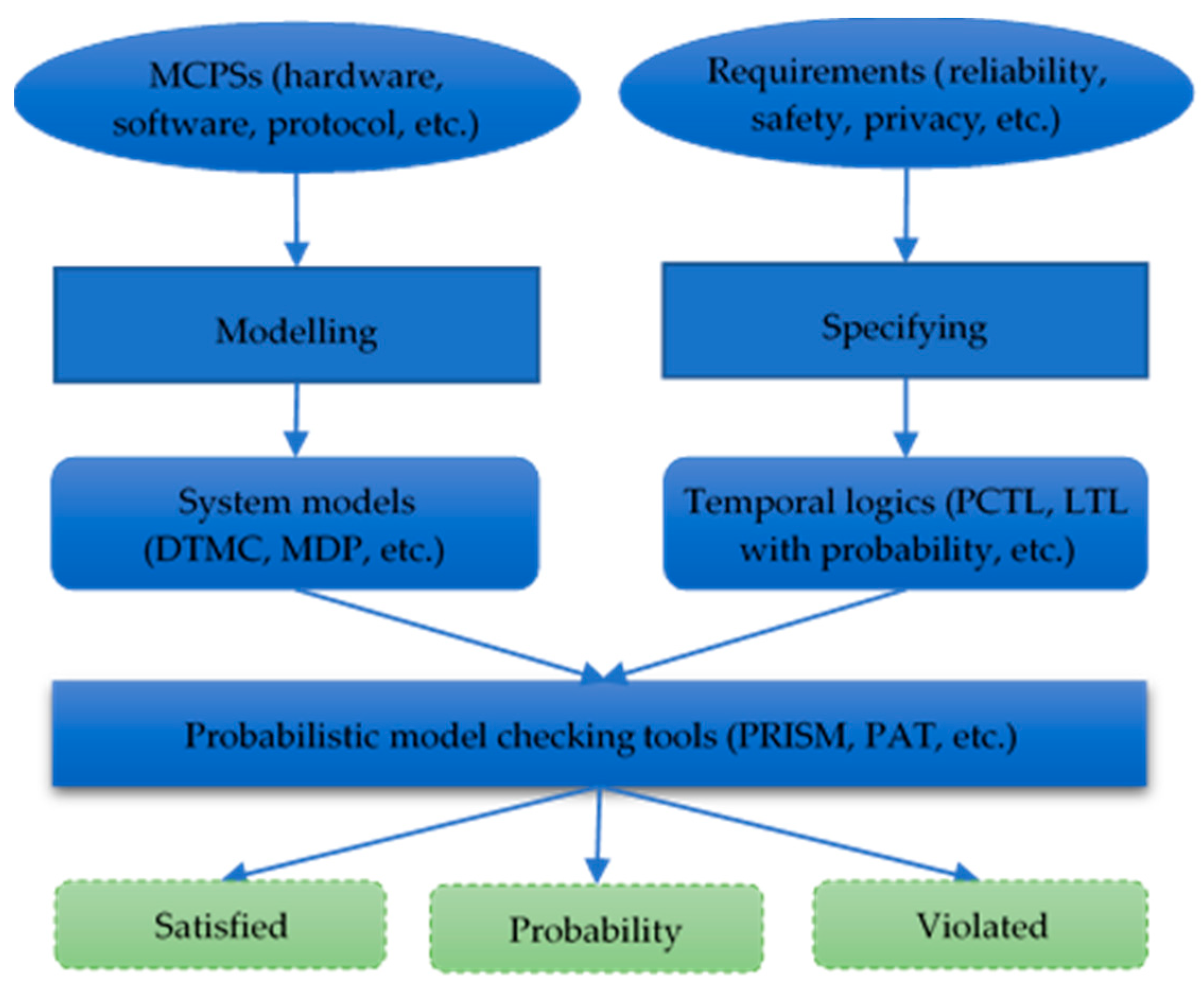
:1. Introduction
1.1. Related Works
1.1.1. Accurate Approach
1.1.2. Approximate Approach
1.2. Our Contribution
1.3. Outline of the Paper
2. Preliminaries
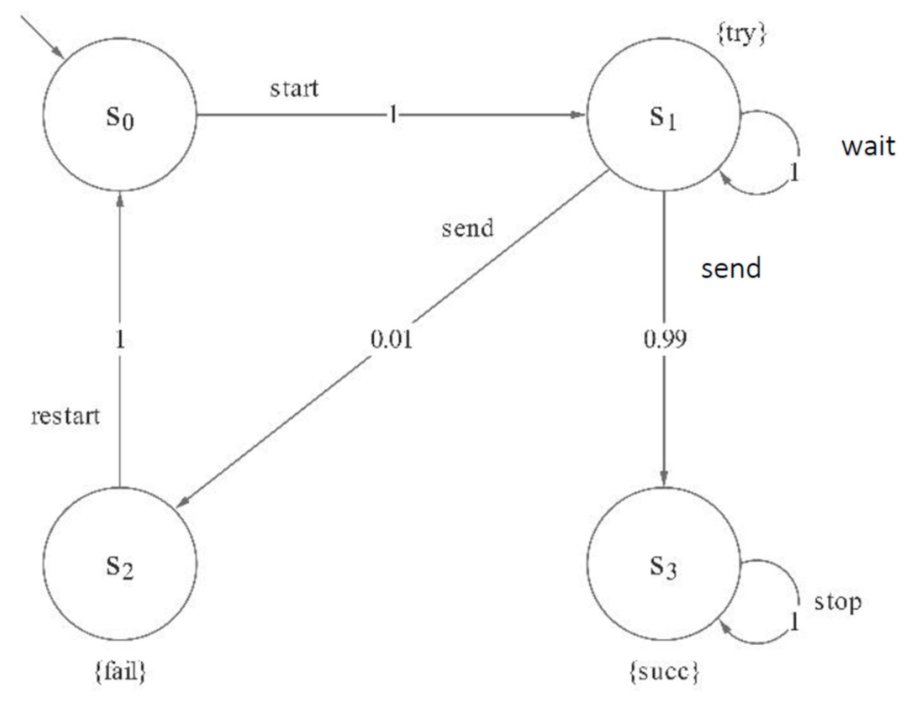
2.1. MDP
2.2. Probabilistic Computation Tree Logic
2.3. Genetic Algorithm
| Algorithm 1. Standard Genetic algorithm. |
| START |
| Generate the initial population |
| Compute fitness |
| REPEAT |
| Selection |
| Crossover |
| Mutation |
| Compute fitness |
| UNTIL population has converged |
| STOP |
3. Counterexample Generation with Heuristic Genetic Algorithm
3.1. Counterexample Represented by Diagnostic Subgraph
3.2. Genetic Algorithm with Heuristic (HGA)
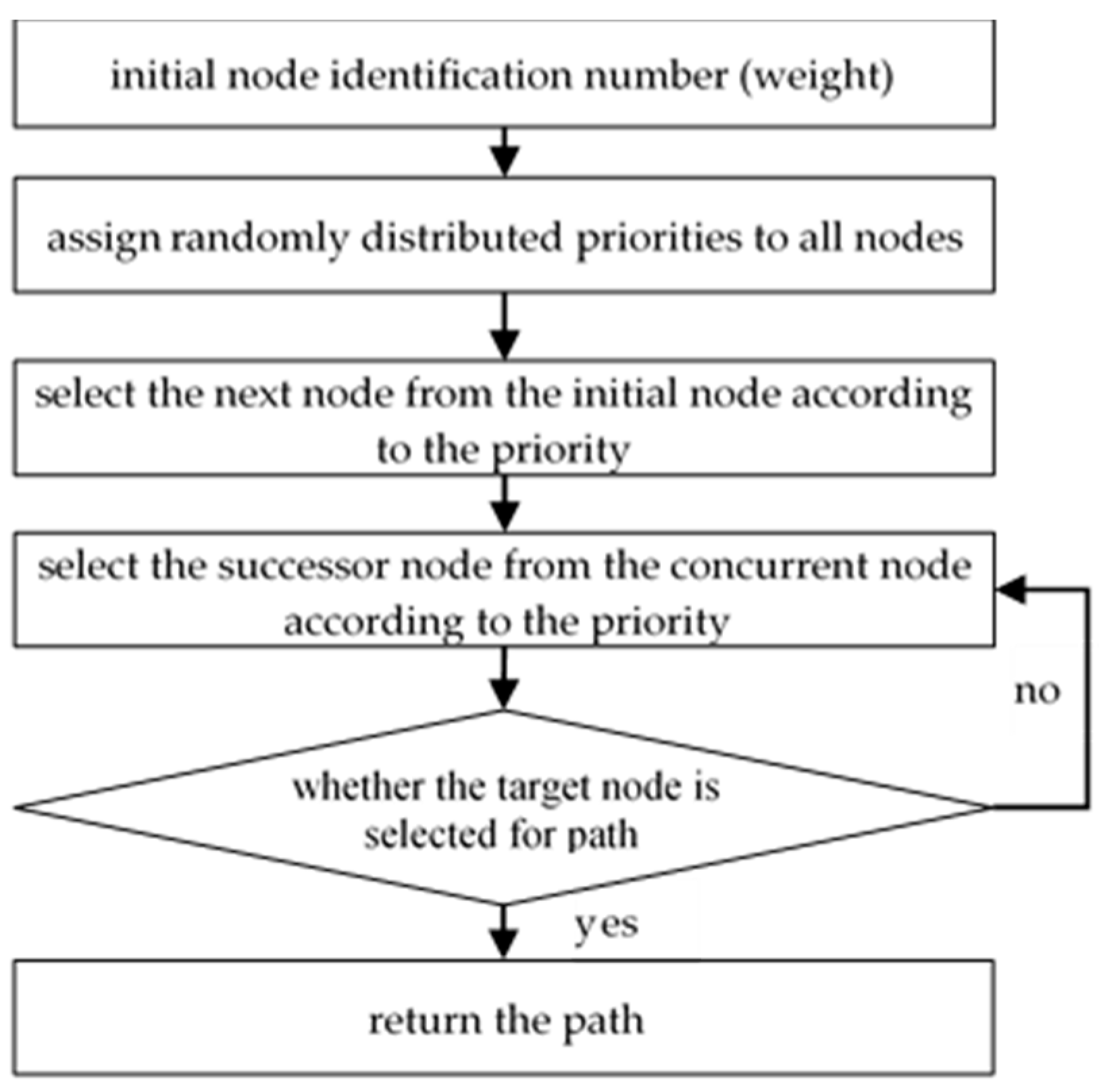
3.2.1. Coding the Path
3.2.2. Fitness Function
3.2.3. Heuristic Crossover Operator
3.2.4. Mutation Operator
3.3. Generating Counterexample with HGA
| Algorithm 2. Counterexample generation for MDP with HGA. |
| Step1: Initialize R and X as an empty set, respectively, that is, without edges and nodes. |
| Step2: Generate a diagnostic path by HGA in Section 3.2 |
| Step3: Replace diagnostic path with the sequence in the AND/OR tree |
| Step4: If R is empty, then directly add the nodes and edges in the and go to step 8. |
| Step5: Determine whether the longest prefix in already exists in R, starting from the initial node . |
| Step6: Add the remainder of to the last node in the longest prefix. |
| Step7: Assign mark to each node in R from the bottom up, where is the probability of each node |
| Step8: If a node in is an AND node, then its probability value is the sum of the child-nodes’ value. |
| Step9: If a node in is an OR node, then its probability value is the maximum of the child-nodes’ value. |
| Step10: If holds, return the counterexample. |
| Step11: Go to Step2 |
3.4. An Example
4. Experimentation
4.1. Dynamic Power Management
4.2. Synchronous Leader Election Protocol
4.3. Zeroconf Protocol
4.4. Bounded Retransmission Protocol
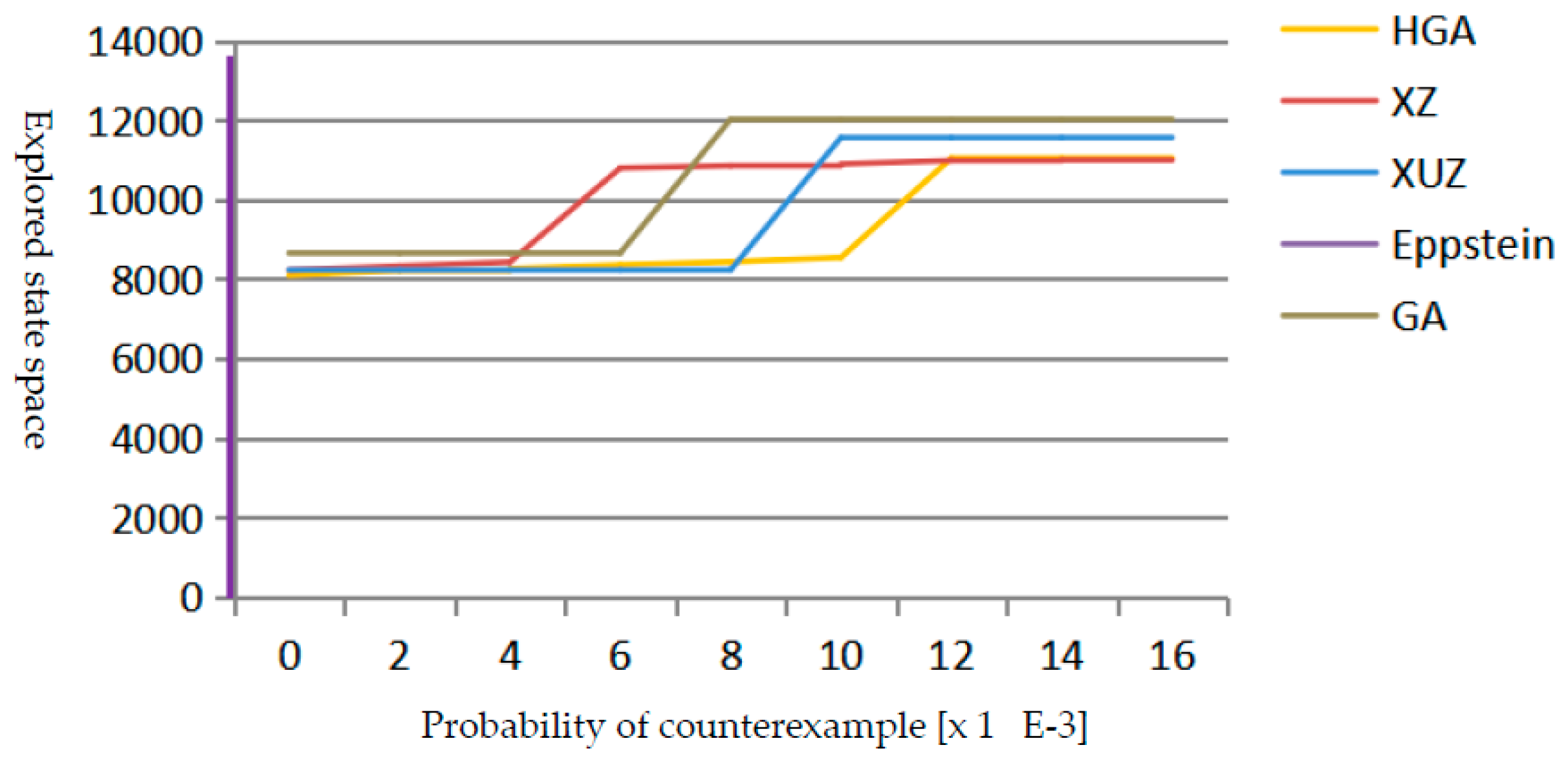
4.5. Analysis
5. Conclusions
Author Contributions
Funding
Acknowledgments
Conflicts of Interest
Abbreviations
| Full Name | Abbreviation |
| Micro-scale Cyber-Physical Systems | MCPSs |
| Micro-scale Cyber-Physical System | MCPS |
| Discrete-time Markov Chains | DTMCs |
| Markov Decision Processes | MDPs |
| Probabilistic tic Timed Automata | PTA |
| Probabilistic Computation Tree Logic | PCTL |
| Liner Temporal logic | LTL |
| Probabilistic Timed Computation Tree Logic | PTCTL |
| Bounded Model Checking | BMC |
| Best-Frist | BF |
| Genetic Algorithm | GA |
| Heuristic Genetic Algorithm | HGA |
| Bounded Retransmission Protocol | BRP |
| Continuous-time Markov Decision Processes | CTMDPs |
| Probabilistic Hybrid Automata | PHA |
| Continuous-time Stochastic Logic | CSL |
References
- Lee, E.A.; Seshia, S.A. Introduction to Embedded Systems, a Cyber-Physical Systems Approach, 2nd ed.; MIT Press: Cambridge, MA, USA, 2017. [Google Scholar]
- Mulet Alberola, J.A.; Fassi, I. Cyber-Physical Systems for Micro-/Nano-assembly Operations: A Survey. Curr. Robot. Rep. 2021, 2, 33–41. [Google Scholar] [CrossRef]
- Trunzer, E.; Vogel-Heuser, B.; Chen, J.-K.; Kohnle, M. Model-Driven Approach for Realization of Data Collection Architectures for Cyber-Physical Systems of Systems to Lower Manual Implementation Efforts. Sensors 2021, 21, 745. [Google Scholar] [CrossRef] [PubMed]
- Wang, Y.; Zarei, M.; Bonakdarpoor, B.; Pajic, M. Probabilistic conformance for cyber-physical systems. In Proceedings of the ACM/IEEE 12th International Conference on Cyber-Physical Systems (ICCPS’21), Association for Computing Machinery, New York, NY, USA, 19–21 May 2021; pp. 55–66. [Google Scholar] [CrossRef]
- Clarke, E.M.; Henzinger, T.A.; Veith, H.; Bloem, R. (Eds.) Handbook of Model Checking; Springer: Cham, Switzerland, 2018. [Google Scholar]
- Kwiatkowska, M.; Norman, G.; Parker, D. PRISM 4.0: Verification of probabilistic real-time systems. In International Conference on Computer Aided Verification; Springer: Berlin/Heidelberg, Germany, 2011; pp. 585–591. [Google Scholar]
- Liu, Y.; Sun, J.; Dong, J.S. PAT 3: An extensible architecture for building multi-domain model checkers. In Proceedings of the 2011 IEEE 22nd International Symposium on Software Reliability Engineering, Hiroshima, Japan, 29 November 2011; pp. 190–199. [Google Scholar]
- Lacerda, B.; Faruq, F.; Parker, D.; Hawes, N. Probabilistic Planning with Formal Performance Guarantees for Mobile Service Robots. Int. J. Robot. Res. 2019, 38, 1098–1123. [Google Scholar] [CrossRef]
- Pfeffer, A.; Wu, C.; Fry, G.; Lu, K.; Marotta, S.; Reposa, M.; Shi, Y.; Kumar, T.S.; Knoblock, C.A.; Parker, D.; et al. Software Adaptation for an Unmanned Undersea Vehicle. IEEE Softw. 2019, 36, 1–96. [Google Scholar] [CrossRef]
- Henze, R.; Mu, C.; Puljiz, M.; Henze, R.; Mu, C.; Puljiz, M.; Kamaleson, N.; Huwald, J.; Haslegrave, J.; di Fenizio, P.S.; et al. Multi-scale Stochastic Organization-oriented Coarse-graining Exemplified on the Human Mitotic Checkpoint. Sci. Rep. 2019, 9, 3902. [Google Scholar] [CrossRef]
- Chen, T.; Diciolla, M.; Kwiatkowska, M.; Mereacre, A. Quantitative Verification of Implantable Cardiac Pacemakers. In Proceedings of the 33rd IEEE Real-Time Systems Symposium (RTSS’12), San Juan, PR, USA, 4–7 December 2012; pp. 263–272. [Google Scholar]
- Bernardeschi, C.; Domenici, A.; Masci, P. A PVS-Simulink Integrated Environment for Model-Based Analysis of Cyber-Physical Systems. IEEE Trans. Softw. Eng. 2018, 44, 512–533. [Google Scholar] [CrossRef]
- Češka, M.; Hensel, C.; Junges, S.; Katoen, J.P. Counterexample-guided inductive synthesis for probabilistic systems. Form. Asp. Comput. 2021, 33, 637–667. [Google Scholar] [CrossRef]
- Lal, R.; Prabhakar, P. Counterexample guided abstraction refinement for polyhedral probabilistic hybrid systems. ACM Trans. Embed. Comput. 2019, 18, 1–23. [Google Scholar] [CrossRef]
- Gao, M.; Wang, K.; He, L. Probabilistic model checking and scheduling implementation of an energy router system in energy Internet for green cities. IEEE Trans. Ind. Inform. 2018, 14, 1501–1510. [Google Scholar] [CrossRef]
- Liu, Y.; Ma, L.; Zhao, J. Secure deep learning engineering: A road towards quality assurance of intelligent systems. In Proceedings of the 21st International Conference on Formal Engineering Methods, Shenzhen, China, 5–9 November 2019; Springer: Cham, Switzerland, 2019; pp. 3–15. [Google Scholar]
- Han, T.; Katoen, J.P. Counterexamples in probabilistic model checking. In International Conference on Tools and Algorithms for the Construction and Analysis of Systems; Springer: Berlin/Heidelberg, Germany, 2007; pp. 72–86. [Google Scholar]
- Han, T.; Katoen, J.P.; Damman, B. Counterexample generation in probabilistic model checking. IEEE Trans. Softw. Eng. 2009, 35, 241–257. [Google Scholar]
- Daws, C. Symbolic and parametric model checking of discrete-time Markov chains. In International Colloquium on Theoretical Aspects of Computing; Springer: Berlin/Heidelberg, Germany, 2005; pp. 280–294. [Google Scholar]
- Andrés, M.E.; D’Argenio, P.; van Rossum, P. Significant diagnostic counterexamples in probabilistic model checking. In Haifa Verification Conference; Springer: Berlin/Heidelberg, Germany, 2008; pp. 129–148. [Google Scholar]
- Jansen, N.; Abrah´am, E.; Katelaan, J.; Wimmer, R.; Katoen, J.P.; Becker, B. Hierarchical counterexamples for discrete-time Markov chains. In International Symposium on Automated Technology for Verification and Analysis; Springer: Berlin/Heidelberg, Germany, 2011; pp. 443–452. [Google Scholar]
- Hermanns, H.; Wachter, B.; Zhang, L. Probabilistic CEGAR. In Proceedings of the International Conference on Computer Aided Verification, Princeton, NJ, USA, 2 January 2018; pp. 162–175. [Google Scholar]
- Chadha, R.; Viswanathan, M. A counterexample-guided abstraction-refinement framework for Markov decision processes. ACM Trans. Comput. Log. 2010, 12, 1–45. [Google Scholar] [CrossRef] [Green Version]
- Češka, M.; Hensel, C.; Junges, S.; Katoen, J.P. Counterexample-driven synthesis for probabilistic program sketches. In International Symposium on Formal Methods; Springer: Cham, Switzerland, 2019; pp. 101–120. [Google Scholar]
- Jansen, N.; Abraham, E.; Zajzon, B.; Wimmer, R.; Schuster, J.; Katoen, J.P.; Becker, B. Symbolic counterexample generation for discrete-time Markov chains. In International Workshop on Formal Aspects of Component Software; Springer: Berlin/Heidelberg, Germany, 2012; pp. 134–151. [Google Scholar]
- Jansen, N.; Wimmer, R.; Abrah´am, E.; Zajzon, B.; Katoen, J.P.; Becker, B.; Schuster, J. Symbolic counterexample generation for large discrete-time Markov chains. Sci. Comput. Program. 2014, 91, 90–114. [Google Scholar] [CrossRef]
- Wimmer, R.; Jansen, N.; Ábrahám, E.; Becker, B.; Katoen, J.P. Minimal critical subsystems for discrete-time Markov models. In Proceedings of the International Conference on Tools and Algorithms for the Construction and Analysis of Systems, Tallinn, Estonia, 24 March 2012; Springer: Berlin/Heidelberg, Germany, 2012; pp. 299–314. [Google Scholar]
- Wimmer, R.; Becker, B.; Jansen, N.; Abrahám, E.; Katoen, J.P. Minimal Critical Subsystems as Counterexamples for omega-Regular DTMC Properties. In MBMV; Kovač: Hamburg, Germany, 2012; pp. 169–180. [Google Scholar]
- Aljazzar, H.; Leue, S. Directed explicit state-space search in the generation of counterexamples for stochastic model checking. IEEE Trans. Softw. Eng. 2010, 36, 37–60. [Google Scholar] [CrossRef] [Green Version]
- Ma, Y.; Cao, Z.; Liu, Y. A PSO-Based CEGAR Framework for Stochastic Model Checking. Int. J. Softw. Eng. Knowl. Eng. 2019, 29, 1465–1495. [Google Scholar] [CrossRef]
- Zheng, T.; Liu, Y. Genetic Algorithm for Generating Counterexample in Stochastic Model Checking. In Proceedings of the 2018 VII International Conference on Network, Communication and Computing, Taipei City, Taiwan, 14–16 December 2018; pp. 92–96. [Google Scholar]
- Segala, R.; Lynch, N. Probabilistic simulations for probabilistic processes. Nord. J. Comput. 1995, 2, 250–273. [Google Scholar]
- Katoch, S.; Chauhan, S.S.; Kumar, V. A review on genetic algorithm: Past, present, and future. Multimed. Tools Appl. 2021, 80, 8091–8126. [Google Scholar] [CrossRef] [PubMed]
- Beke, L.; Weiszer, M.; Chen, J. A Comparison of Genetic Representations for Multi-objective Shortest Path Problems on Multigraphs. In Proceedings of the European Conference on Evolutionary Computation in Combinatorial Optimization (Part of EvoStar), Seville, Spain, 15–17 April 2020; pp. 35–50. [Google Scholar]
- Ghasemishabankareh, B.; Ozlen, M.; Li, X.; Deb, K. A genetic algorithm with local search for solving single-source single-sink nonlinear non-convex minimum cost flow problems. Soft Comput. 2020, 24, 1153–1169. [Google Scholar] [CrossRef]
- Benini, L.; Bogliolo, A.; Paleologo, G.A.; De Micheli, G. Policy optimization for dynamic power management. IEEE Trans. Comput. Aided Des. Integr. Circuits Syst. 1999, 18, 813–833. [Google Scholar] [CrossRef]
- Aljazzar, H.; Leitner-Fischer, F.; Leue, S. Dipro-a tool for probabilistic counterexample generation. In International SPIN Workshop on Model Checking of Software; Springer: Berlin/Heidelberg, Germany, 2016; pp. 183–187. [Google Scholar]
- Arnaboldi, L.; Czekster, R.M.; Morisset, C.; Metere, R. Modelling Load-Changing Attacks in Cyber-Physical Systems. Electron. Notes Theor. Comput. Sci. 2020, 353, 39–60. [Google Scholar] [CrossRef]
- Itai, A.; Rodeh, M. Symmetry breaking in distributed networks. Inf. Comput. 1990, 88, 60–87. [Google Scholar] [CrossRef] [Green Version]
- Srinivasan, S.; Kandukoori, R. A synod based deterministic and indulgent leader election protocol for asynchronous large groups. Int. J. Parallel Emergent Distrib. Syst. 2021, 1–28. [Google Scholar] [CrossRef]
- Norman, G.; Parker, D.; Zou, X. Verification and control of partially observable probabilistic systems. Real-Time Syst. 2017, 53, 354–402. [Google Scholar] [CrossRef] [Green Version]
- Kwiatkowska, M.; Norman, G.; Parker, D.; Sproston, J. Performance analysis of probabilistic timed automata using digital clocks. Form. Methods Syst. Des. 2006, 29, 33–78. [Google Scholar] [CrossRef] [Green Version]
- Aarts, F.; Kuppens, H.; Tretmans, J.; Vaandrager, F.; Verwer, S. Learning and testing the bounded retransmission protocol. In Proceedings of the International Conference on Grammatical Inference, College Park, MD, USA, 12–15 September 2012; pp. 4–18. [Google Scholar]
- Guo, X.; Kurushima, A.; Piunovskiy, A.; Zhang, Y. On gradual-impulse control of continuous-time Markov decision processes with exponential utility. Adv. Appl. Probab. 2021, 53, 301–334. [Google Scholar] [CrossRef]
- Sproston, J. Verification and control for probabilistic hybrid automata with finite bisimulations. J. Log. Algebraic Methods Program. 2019, 103, 46–61. [Google Scholar] [CrossRef]


| K | 2 | 4 |
|---|---|---|
| States | 77,279 | 276,781 |
| Transitions | 180,442 | 640,721 |
| Time | 24.868 | 77.430 |
| Memory | 3584.0 | 11,878.4 |
| K | Probability | Eppstein | XUZ | GA | HGA |
|---|---|---|---|---|---|
| 2 | 0.01 | 19.076 | 17.161 | 16.105 | 15.176 |
| 0.04 | 169.06 | 165.090 | 156.223 | 105.103 | |
| 0.08 | 909.082 | 801.214 | 601.31 | 520.282 | |
| 0.1 | 2198.009 | 1996.071 | 1077.56 | 809.072 | |
| 4 | 0.01 | 93.040 | 105.943 | 37.09 | 29.235 |
| 0.04 | 786.047 | 518.177 | 509.43 | 435.034 | |
| 0.08 | 5963.085 | 4163.076 | 2607.38 | 1998.089 | |
| 0.1 | Failed | Failed | 5901.92 | 4076.92 |
| K | Probability | Eppstein | XUZ | GA | HGA |
|---|---|---|---|---|---|
| 2 | 0.01 | 797.9 | 702.8 | 699.4 | 690.2 |
| 0.04 | 3798.4 | 3301.7 | 2863.5 | 2831.3 | |
| 0.08 | 7802.2 | 7032.9 | 5051.2 | 4960.3 | |
| 0.1 | 18,915.6 | 16,970.3 | 10,967.9 | 9818.9 | |
| 4 | 0.01 | 7849.2 | 7649.3 | 7734.6 | 5782.34 |
| 0.04 | 37,851.7 | 37,091.8 | 15,736.6 | 9825.4 | |
| 0.08 | 87,869.7 | 85,981.8 | 36,751.5 | 17,838.3 | |
| 0.1 | Failed | Failed | 99,302.2 | 48,804.2 |
| N | 640 | 3200 |
|---|---|---|
| States | 103,962 | 518,682 |
| Transitions | 139,888 | 697,968 |
| Time | 347.055 | 5023.233 |
| Memory | 4403.2 | 20,992.0 |
| N | Probability | Eppstein | XUZ | GA | HGA |
|---|---|---|---|---|---|
| 640 | 0.01 | 132.721 | 120.835 | 111.443 | 109.234 |
| 0.04 | 633.893 | 626.542 | 496.856 | 409.764 | |
| 0.08 | 5328.984 | 4996.132 | 1975.362 | 1153.762 | |
| 0.10 | Failed | Failed | 4206.716 | 2043.571 | |
| 3200 | 0.005 | 1402.754 | 1603.239 | 1085.234 | 987.365 |
| 0.008 | 5405.326 | 5564.271 | 2354.331 | 1801.259 | |
| 0.016 | Failed | Failed | 5979.845 | 2969.267 | |
| 0.02 | Failed | Failed | Failed | 8597.813 |
| N | Probability | Eppstein | XUZ | GA | HGA |
|---|---|---|---|---|---|
| 640 | 0.01 | 13,009.5 | 13,447.4 | 12,950.1 | 12,908.3 |
| 0.04 | 23,768.1 | 24,647.8 | 23,840.4 | 21,987.2 | |
| 0.08 | 514,153.4 | 528,356.3 | 49,453.2 | 77,623.2 | |
| 0.10 | Failed | Failed | Failed | 893,615.8 | |
| 3200 | 0.005 | 549,063.4 | 43,252.3 | 30,432.2 | 29,987.5 |
| 0.008 | 793,109.2 | 797,602.6 | 618,023.1 | 50,568.2 | |
| 0.016 | Failed | Failed | 896,581.1 | 93,298.4 | |
| 0.02 | Failed | Failed | Failed | 897,536.8 |
Publisher’s Note: MDPI stays neutral with regard to jurisdictional claims in published maps and institutional affiliations. |
© 2021 by the authors. Licensee MDPI, Basel, Switzerland. This article is an open access article distributed under the terms and conditions of the Creative Commons Attribution (CC BY) license (https://creativecommons.org/licenses/by/4.0/).
Share and Cite
Liu, Y.; Ma, Y.; Yang, Y.; Zheng, T. Counterexample Generation for Probabilistic Model Checking Micro-Scale Cyber-Physical Systems. Micromachines 2021, 12, 1059. https://doi.org/10.3390/mi12091059
Liu Y, Ma Y, Yang Y, Zheng T. Counterexample Generation for Probabilistic Model Checking Micro-Scale Cyber-Physical Systems. Micromachines. 2021; 12(9):1059. https://doi.org/10.3390/mi12091059
Chicago/Turabian StyleLiu, Yang, Yan Ma, Yongsheng Yang, and Tingting Zheng. 2021. "Counterexample Generation for Probabilistic Model Checking Micro-Scale Cyber-Physical Systems" Micromachines 12, no. 9: 1059. https://doi.org/10.3390/mi12091059
APA StyleLiu, Y., Ma, Y., Yang, Y., & Zheng, T. (2021). Counterexample Generation for Probabilistic Model Checking Micro-Scale Cyber-Physical Systems. Micromachines, 12(9), 1059. https://doi.org/10.3390/mi12091059