Abstract
Tree growth and survival predominantly depends on edaphic and climatic conditions, thus climate change will inevitably influence forest health and growth. It will affect forests directly, for example, through extended periods of drought, and indirectly, such as by affecting the distribution and abundance of forest pathogens and pests. Developing ways of early detection and monitoring of tree stress is crucial for effective protection of forest stands. Thermography is one of the techniques that can be used for monitoring changes in the physiological state of plants; however, in forestry, it has not been widely tested or utilized. The main challenge rises from the need for high spatial resolution data. Newly emerging technologies, such as unmanned aerial vehicles (UAVs) could aid in provision of the required data. However, their main constraint is the limited payload, requiring the use of miniature sensors. This paper investigates whether a miniature microbolometer thermal camera, designed for a UAV platform, can provide reliable canopy temperature measurements of conifers. Furthermore, it explores whether there is a distinction in whole canopy temperature between the control and the stressed trees, assessing the potential of low-cost thermography for investigating stress in conifers. Two experiments on young larch trees, with induced drought stress, were performed. The plants were imaged in a greenhouse setting, and readings from a set of thermocouples attached to the canopy were used as a method of validation. Following calibration and a basic normalization for background radiation, both the spatial and temporal variation of canopy temperature was well characterized. Very mild stress did not exhibit itself, as the temperature readings for both stressed and control plants were similar. However, with a higher stress level, there was a clear distinction (temperature difference of 1.5 °C) between the plants, showing potential for using low-cost sensors to investigate tree stress.
1. Introduction
Tree growth and survival predominantly depends on edaphic and climatic conditions, which influence processes such as photosynthesis and respiration. Thus, gradual global warming, with consequent changes to other climate variables such as rainfall, humidity and weather patterns, will inevitably influence forest health and tree growth []. Higher carbon dioxide concentrations, and the resulting lengthening of the growing season should increase the productivity of trees, if water and nutrients do not become limiting factors []. However, according to model simulations, a decrease in precipitation in the south of Europe is expected, particularly in the summer period, whilst over much of northern Europe an increase in precipitation is predicted [,,]. For instance, it is suggested that, under the medium emissions scenario (scenario A1B within the Special Report on Emission Scenario, SRES), rainfall over much of the UK will increase by up to 33% in winter months and decrease by as much as 40% in summer months by the 2080s, relative to the 1961–1990 baseline []. Such changing rainfall patterns are likely to increase the frequency of surface water droughts, but also increase the risk of extreme precipitation and flooding [,,].
Climate change will also indirectly affect the distribution and abundance of forest pathogens and pests, as well as the severity of tree diseases. The predicted temperature rise and longer growing season will generally favor insect population growth and expansion [,], whilst moister conditions, with greater water table fluctuations, will benefit pathogens []. The extended periods of droughts with climate change are likely to bring an increase in trees’ vulnerability to attack []. Developing ways of monitoring tree stress is therefore crucial for effective protection of forest stands. In response to changing tree health status, forest management strategies can be adapted to help mitigate effects of climate change, such as pests and disease outbreaks. Thermography is one of the techniques that can be used for monitoring changes in the physiological state of plants; however, in forestry, it has not been widely utilized or tested.
Leaf temperature is primarily determined by the rate of transpiration. As plants transpire, water loss through evaporative cooling reduces leaf temperature []. Conversely, plants under water stress tend to transpire less due to stomatal closure, leading to an increase in leaf and canopy temperature and reduction in photosynthetic activity []. Therefore, leaf temperature can be an indicator of water availability. With the onset of severe water stress, a general disruption of metabolism develops, which is signaled by high rates of respiration. The closure of stomatal apertures is a defense mechanism, which not only helps reduce water losses, but also prevents the entry of microbes and host tissue colonization. The resultant increase in leaf and canopy temperature can often be detected by thermal imaging at the leaf level at an early stage of infection [,].
In agriculture, much work has been done on relating leaf temperature to water stress. At canopy level, several methods utilizing knowledge on environmental factors (such as air temperature, humidity, radiation and wind speed) were developed to estimate stomatal conductance and water content using thermography [,,]. As an alternative, thermal “stress indices” were created, aiming to normalize the results for environmental variation. Canopy temperature depression (CTD) is the most straightforward of the indices; it normalizes canopy temperature with reference to air temperature, and is calculated as Tcanopy – Tair []. However, it depends on weather conditions, and thus can only be used in climates where weather conditions vary little between consecutive days []. The crop water stress index (CWSI) is a drought stress index, which introduces a non-water-stressed baseline (representing a crop transpiring at a maximal rate) and a non-transpiring upper baseline (representing a dry crop with closed stomata) [,]. There are different approaches for calculation of CWSI, namely analytical, empirical and direct; a review of these approaches can be found in Maes et al. []. Similarly, the stomatal conductance indices (Ig and I3) utilize “wet” and “dry” reference surfaces to reduce the sensitivity to environmental variations [].
The thermal stress indices have been widely and successfully applied to agricultural crops [,,]. However, the use of thermography for investigation of water stress in trees has been predominantly limited to orchards [,,]. Using thermal imagery, noticeable differences in canopy temperature between treatments of persimmon trees were detected, whilst in citrus the relationship between crown temperature and plant water stress differed in each experimental season []. Within a heterogeneous olive orchard, good correlation between estimated and field-measured canopy conductance values was achieved by Berni et al. []. Similarly, the CWSI, modeled for water-deficient and well-irrigated olive trees, correlated well with the measured water potential, as well as the canopy conductance []. Relationships between canopy temperature, and stomatal conductance and water potential, were also found in almond trees []; furthermore, it was suggested that the intra-crown temperature variability could also be used for water stress detection.
In forestry, thermography so far has been used to analyze drought tolerance of several deciduous tree species in a mixed forest stand [] and of Scots pine seedlings from different provenances [] to assist forest planning in light of changing climatic conditions. Scherrer et al. [] recorded noticeable differences between investigated species, ranking them according to their resistance. With ongoing drought, they also observed a divergence in mean relative (to air) canopy temperature readings between “dry” and “moist” sites, but could not attribute them to differences in soil water potential. Grant et al. [], using thermal imagery, monitored leaf physiology of cork oak under varying water regimes (80%, 100% and 120% of natural precipitation). Following a year of treatment, the well-watered leaves were significantly cooler than those with natural or reduced precipitation levels. On a larger scale, MODIS land surface temperature was used with monthly water balance to derive a forest vulnerability index []. Nevertheless, the application of thermography to investigate stress in forest species, especially conifers, requires further exploration to assess its feasibility as a reliable monitoring technique. Conifers represent particularly challenging targets for remote sensing analysis, mainly due to their structural features, for example, narrow needle leaves. With the exception of [,,], thermography of conifer trees still remains almost unreported in the literature; therefore, the investigation of stress responses in the temperature domain is largely lacking. In Kim et al. [], the daily and sub-daily mean canopy temperatures extracted from uncorrected imagery were shown to be related to climatic and soil variables, whilst Smigaj et al. [] found a correlation between disease progression and canopy temperature increase. However, neither of these studies validated the retrieved canopy temperatures against ground measurements. Seidel et al. [] used thermocouples attached to needles to derive their apparent emissivity, but did not utilize them in further measurements.
The main challenge for using thermal remote sensing approaches for forest health monitoring arises from the need for high spatial resolution data to identify individual trees or to monitor areas of fragmented forest cover. Newly emerging technologies, such as small unmanned aerial vehicles (UAVs) could significantly aid in provision of the required data. However, the main constraint of UAV platforms is the limited payload they offer, requiring the use of miniature sensors. Thermal sensors would traditionally utilize quantum detectors, offering short (sub-nanosecond) response times and very high sensitivities. However, to reduce thermal generation of charge carriers and thermal noise, they require an external cooling system, making them bulky and expensive. The development of sensors based on thermal detectors has allowed for significant miniaturization of thermal cameras. They tend to have slower response times and are less sensitive than quantum detectors, but do not need any cooling element. This makes them less expensive and more competitive, as well as allowing for miniaturization of the sensor. Lack of a cooling system results in a low signal to noise ratio, but makes such sensors sufficiently lightweight for inclusion as part of a UAV payload. Uncooled thermal imagers are severely degraded by the spatial non-uniformity noise, which is defined as spatially heterogeneous response of the camera to uniform incoming radiation []. The non-uniformity noise has a fixed spatial structure, but its intensity varies over time due to instability in the camera temperature [,]. It is particularly severe in microbolometer sensors because the infrared detector tends to drift over time; temperature variations result in a different thermal drift among the detector elements, exacerbating the effects of the non-uniformity [,]. Thermal imagers provide an internal system correcting for the drift and non-uniformity caused by the drift. However, as this system is located between the detector and the optics (which are also imperfect), some non-uniformity across the image is expected to remain [].
This study investigates whether a low-cost miniature thermal camera, destined to be used on a UAV platform, is capable of providing reliable canopy temperature measurements of conifers. For this purpose, the temporal change and spatial variation of canopy temperature in conifer trees is monitored in a greenhouse setting. Furthermore, the paper explores whether there is a distinction in whole canopy temperature between the control and the stressed trees, assessing the potential of low-cost thermography for investigating tree stress in conifers.
2. Materials and Methods
2.1. Thermal Camera Specifications and Calibration
The thermal sensor used for this study is a weight-optimized Optris® PI-450 longwave infrared camera (Optris GmbH, Berlin, Germany), equipped with a 38° × 29° field-of-view lens and manual focus. It utilizes uncooled microbolometers arranged into a Focal Plane Array with optical resolution of 382 × 288 pixels. The camera’s internal mechanical calibration device was set to flag in front of the detector every 12 s to correct for the thermal drift and non-uniformity caused by the drift. The sensor operates in a spectral range of 7.5–13 µm and a temperature range of 20–900 °C (thermal sensitivity: 40 mK, accuracy: ±2 °C or ±2%, whichever is larger). Prior to such sensor use, its performance in obtaining reliable temperature measurements across the whole lens has to be determined. This is crucial for quantitative use of the camera, especially when applied to plant sciences, where differences in temperature are usually small.
The Optris® thermal camera was therefore calibrated in laboratory conditions against a thermally controlled flat plate blackbody radiation source (ISDC’s IR-160, εBB = 0.96), ensuring the camera’s field-of-view was fully covered by the blackbody. The emitter has a size of 12′′× 12′′, temperature resolution of 0.1 °C (calibration accuracy: ±0.2 °C) with short and long-term stability of ±0.2 °C and ±0.1 °C, respectively. It operates in the temperature range of ambient to 350 °C and spectral range of 1–99 µm. The blackbody source used in this study is heated by means of a resistive-heating element, which is designed to provide uniform heating of the entire surface area. To ensure even distribution of the power to the entire surface (that is proper uniformity), after each temperature setting change the system was given 30 min to stabilize before measurements were made.
Thermal cameras can be radiometrically corrected by quantitatively relating their output to source radiance or temperature. Typically, this would be performed by measuring the output digital numbers while the camera views one or more blackbody sources []. In this study, the non-uniformity across the image was corrected using a two-point calibration technique [], which requires measuring a blackbody at two distinct and known temperatures. If the output digital numbers are linearly related to the input radiance, then for a given wavelength:
where R is spectral radiance emitted by target surface, G is spectral response (gain) of the sensor, S are digital numbers recorded by the sensor, O is spectral radiance emitted by sensor’s internal parts (offset), and λ is wavelength. If the radiances of two blackbodies at different known temperatures (“cold” and “hot”) are given by:
where Pc and Ph are band-integrated “cold” and “hot” blackbody radiances, respectively; Tc and Th are their temperatures; and P is Planck blackbody radiance. Then, by measuring image intensities, there is enough information to solve Equation (1) for gain and offset parameters:
This equation was then adjusted to account for the emissivity of the blackbody source (εBB):
As Equation (1) is sensitive to any nonlinearity between the input radiance and output data numbers, it was first ensured the average and pixel level sensor responses were linear in terms of emitted flux versus digitized flux over a range of temperatures at both image and pixel level. Imagery of the blackbody at 298.15 K to 333.15 K was then used to calculate the gain and the bias of each detector across the array. To minimize any temporal differences in temperature offsets recorded within each pixel, averages of 10 consecutive images, taken at 10 s intervals, were used. To check the effectiveness of the derived non-uniformity correction, the offset and gain matrices were applied to a temporal set of the imagery. The camera was set to store one raw image of a blackbody at 298.15 K (25.0 °C) every minute over the course of 109 min. The kinetic temperature values acquired by the camera were computed using an emissivity value for the blackbody of 0.96.
2.2. Plant Preparation and Experiment Design
Twenty specimens of potted two-year-old Japanese larch trees were selected and kept throughout 2016 in an indoor growth room made of glass. The plants were divided into control and drought-stressed groups in August 2016, and since then watered at 2–3 days intervals, with reduced amount provided to the drought group. In control trees, the soil moisture content was aimed to be maintained above 50% (but no more than 80%), whilst, in the drought stress group, between 10% and 30%. The air temperature within the room was set to 16 °C, and for the last month prior to acquiring imagery, temperature varied between 16 and 22 °C as on warm days the cooling system could not retain a constant low temperature.
Two separate pairs of structurally similar trees (one treated, one control) were selected for the experiments conducted on 7 and 10 October 2016, during which the Optris PI-450 thermal camera was used to take images. The first trial involved a moderately stressed tree, whilst the second used a mildly stressed tree; soil moisture measurements (using CS650 soil water content reflectometer, Campbell Scientific, Inc. Logan, UT, USA) prior to commencing imaging showed 7% and 33% moisture levels for the drought-stressed trees, and 48% and 63% for the control trees. The tree stress status was based on the soil moisture measurements and the visual examination of the canopies. The difference in soil moisture between equivalent trees in the two experiments was assumed to be caused by different tree sizes, hence different water consumption.
The experiments were performed in a greenhouse to utilize sunlight; additional light sources were also used to ensure plants were undergoing photosynthesis. Two lamps (400 Watt high pressure sodium system) were attached to the roof of the greenhouse approximately one meter from top of the plants, pointing downwards, directly towards the trees. In this set-up, any shadowing of the lower parts of the trees was only expected to come from overhead branches. To minimize the effects of wall reflectance, immediate surroundings were covered with a uniform, non-reflective black paper. A small calibration target, constructed from high-emissivity carpet underlay foam, was placed alongside the plants.
Direct temperature measurements were performed with type K welded tip fast response thermocouple sensors (conductor diameter of 0.315 mm, accuracy of ±2.2 °C). Each plant had a thermocouple wrapped inside of needle clumps in the upper and lower part of the foliage. The sensors were not firmly attached to needles to avoid causing mechanical damage. The temperature of the air and the calibration target was also monitored using thermocouples. The full set-up is presented in Figure 1. The experiments were undertaken in southern Scotland at 14 and 12 local time on 7 and 10 October 2016. In the case of Experiment 1, the plants were initially imaged under natural light conditions; the experiment lasted 60 min, with lamps turned on between Minutes 8 and 55. Weather conditions remained consistent, with a thick cloud cover obstructing the sun. Experiment 2 lasted 47 min and was performed with the lamps on; on that day, the conditions were variable, with intermittent sunshine and moving, thick clouds. The thermal camera was placed approximately 1.5 m away from the plants and acquired imagery at approximately one-minute intervals. The emissivity of the canopy foliage was assumed to be 0.95 (average leaf emissivity value reported by Jones [], based on a range of plant species).
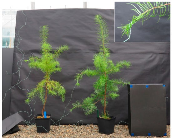
Figure 1.
Experiment 1 set-up with calibration target on the right; thermocouples were wrapped inside of needle clumps, as shown on the inset.
2.3. Calibration Target’s Emissivity Value Retrieval
A MIDAC M2000 series Fourier Transform InfraRed (FTIR) spectrometer (MIDAC, Westfield, MA, USA) was used to perform TIR spectral emissivity measurements of the calibration target’s surface. It is equipped with a mercury cadmium telluride sensor and zinc selenide optics, offering a spectral range of 2–15.4 µm and a selectable resolution of 32–0.5 cm−1. For this study, the spectrometer was set to perform 8 scans with 16 background scans at 2 cm−1 resolution. The calibration of the spectrometer typically involves measuring spectra of reference radiation sources with known temperatures []; in this study a blackbody system built by Electron Systems was utilized, which consists of three blackbodies (εBB = 0.96) , two of which were used and set to 15 °C and 60 °C. The radiance of the target can be described by a basic mathematical model as a function of the spectrum measured by the spectrometer shown in Equation (1), where S would become the uncalibrated energy spectrum measured by the spectrometer. The gain and offset parameters followed the same calculation process, utilizing measurements of the spectral radiance emitted by the two blackbodies. Calibration measurements of the blackbodies along with downwelling radiance (DWR) measurements were performed at regular intervals to account for changes in background radiance and spectrometer temperature. The DWR measurements were acquired using a diffusive gold highly reflective surface (InfraGold panel), with a reported emissivity of less than 0.06 (εG), the radiance of which (RG, as received by the FTIR spectrometer) can be described as:
where RBB(TG,λ) is the radiance emitted by a blackbody at the gold plate’s temperature, RDWR is the downwelling radiance, RA is atmospheric radiance between the plate and spectrometer and τA is the atmospheric transmission between the plate and spectrometer. The measurements were performed over a path shorter than 1 m (from a distance of approximately 30 cm), thus the atmospheric terms τA and RA could be ignored, and the above equation could be rearranged to:
The calculated DWR was subsequently subtracted from upwelling target radiance to isolate target emission and obtain absolute emissivity for each of the measurements:
To ensure the upwelling target radiance was higher than the DWR during the lab measurements, the target samples were heated up (between two metal plates) in a convection oven prior to measurements. Metal plates were used to avoid rapid heat dissipation during transportation of samples. Immediately prior to measurements, the top plate was removed, and then target spectra were collected. In total, eight spectral measurements of the target were used to obtain absolute emissivity. During the measurement, the target was at 29.9 °C to 30.5 °C, whilst the gold panel remained at temperatures from 27.8 °C to 28 °C (measured with a contact thermocouple). The retrieved target’s emissivity within the camera’s spectral range, i.e., 7.5 μm to 13 μm, varied from 0.89 to 0.98, and for further use it was integrated into a single value, denoted as total emissivity, of 0.92. The measurement procedure and the retrieved spectral emissivity are shown in Figure 2.
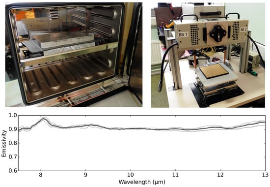
Figure 2.
Emissivity retrieval procedure: heating up of the sample in a convection oven between two metal plates, measurements setup, and average absolute spectral emissivity (black) of the target retrieved from eight spectral measurements (grey).
2.4. Image Processing
The first step of image processing was the application of corrections derived as in Section 2.1 to all acquired thermal imagery. Following this step, the emissivity values of the calibration target and of the canopy foliage were accounted for, resulting in two sets of imagery for further processing.
The signal that reaches the thermal camera is composed of target radiance, but also of background radiance. Background radiance is variable in time, and in indoor environments with emissions from walls, ceiling and other surrounding objects, can introduce a significant error to analysis. To account for changes in background radiance throughout the experiments, the developed calibration target was used. For each of the acquired images, the target’s central 3500 pixels were used to retrieve an average target temperature value, which was compared against the thermocouple measurements. The obtained differences between image and thermocouple readings of the target surface were then subtracted from the camera readings to normalize them for the changes in the background radiance levels.
Following the correction and prior to further analysis, background masks were created by means of temperature thresholding. For each of the experiments, the image with highest plant-to-background temperature contrast (defined as the temperature difference between central part of the stressed canopy and of the background in top part of the image) was used. Based on this image, ten temperature thresholds, one for each set of 25 image rows, were manually chosen to separate plant foliage from the surroundings. The choice of thresholds was aided by comparison with visible imagery, which allowed the number of mixed pixels located at the edges of the canopy to be minimized. Multiple thresholds were required for accurate separation as both the temperature of the background and of the plants depended on the distance from the heat source. The derived masks allowed for extraction of canopy pixels, as presented in Figure 3. To ensure that the selection of canopy pixels was consistent throughout the experiments, the same masks were applied to all imagery within each of the datasets. Furthermore, for a comparison between plants, a second mask (low canopy volume mask) was created excluding image rows in which either of the trees in each of the experiments had a limited foliage; such rows were likely to be affected by mixed pixels (containing the response from both the canopy and the background). Any image row constituting of less than 30 canopy pixels was therefore masked (the resultant mask in shown in Figure 3).
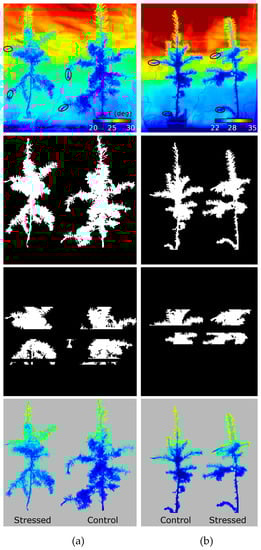
Figure 3.
Canopy pixel extraction for: Experiment 1 (a); and Experiment 2 (b), showing original thermal image, the canopy mask, the low canopy volume mask, and extracted canopy pixels. Black circles indicate regions, where thermocouples were placed.
Another point of interest was the vertical distribution of temperature within the canopies, and how this changed over time. To analyze this, average foliage temperature values for each image row were computed. To minimize large variations in readings between consecutive rows and aid the interpretation, the readings retrieved from all images were smoothed first using Kaiser window smoothing [], with window size of 11 and beta parameter set to 4.
Lastly, average canopy temperature values (following application of the low canopy volume mask) were calculated for each image to compare the thermal response of control and stressed plants over time. The significance of the difference between the canopy temperature means at each time stamp was tested using Welch’s unequal variance t-test [] at 0.01 confidence level (H0 = the true difference in means is equal to zero, null hypothesis rejected at p ≤ 0.01). To provide an indication of the variation of temperature within the canopies, standard deviation was calculated.
3. Results
3.1. Camera Performance in Laboratory Conditions
During camera calibration in laboratory settings, a significant temperature shift was observed over the course of the first 30 min, indicating a need for camera stabilization prior to undertaking any imaging (Figure 4). Moreover, after the readings had stabilized, it was revealed that the sensor overestimated the blackbody’s temperature by over 3.5 K throughout the imaging period. Further investigation of temperature readings at a pixel level showed non-uniformity in the photo response of the detectors in the array; the temperature readings across the imagery varied significantly, with differences exceeding 2 K in some cases (Figure 4). The variation within the response across the imagery was initially assumed to have come from “vignetting” effect, which is the main optical artifact in cameras. It results in a darkening of the image at its periphery due to a transmission coefficient decreasing with increasing distance from the optical axis. However, in the case of the investigated camera, no such pattern was evident. Instead, an increase in recorded temperature value towards the right-hand side of the image was observed. This spatial pattern of offsets remained the same throughout the experiment. We suspect the observed non-uniformity and temperature offset were probably caused by a joint effect of the imperfections of the optics and degradation of the calibration of the sensor.
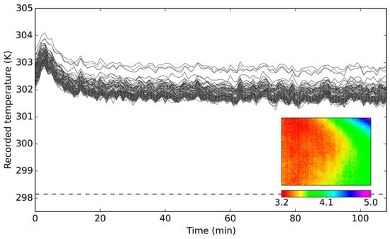
Figure 4.
Temperature readings over time of a blackbody at 298.15 K (dashed line), as recorded by 100 randomly chosen pixels, alongside recorded image offsets from the blackbody temperature (given in K) at Minute 80. The temperature readings were adjusted for the blackbody’s emissivity value (εBB = 0.96). The initial spike in values (first 30 min) was due to the camera warming up period.
The derived non-uniformity correction accounted for the overestimation in the average temperature readings (Figure 5); the imagery was representing the actual blackbody temperature with maximum offsets of mean image temperature of 0.23 K. The variation in temperature readings across the imagery had also been minimized, with 95.4% (2σ) of the pixels falling within ±0.14 K (average across the time series) of the mean temperature reading. The resultant gain and offset matrices were used to correct all acquired thermal imagery. The validity of the derived calibration parameters was subsequently confirmed after six months on the same blackbody source, following a similar measurement set-up.
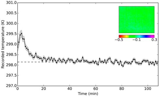
Figure 5.
Corrected mean image temperature of a blackbody at 298.15 K (dashed line), as recorded by a camera over time, alongside recorded image offsets from the blackbody temperature (given in K) at Minute 80. The temperature readings were adjusted for the blackbody’s emissivity value (εBB = 0.96). Shaded areas represent one-sigma standard deviation; the initial spike in values (first 30 min) was due to the camera warming up period.
3.2. Changes in Background Radiation inside the Greenhouse
At the beginning of the Experiment 1, undertaken under cloudy weather conditions, the difference between the calibration panel thermocouple and image measurements was around 2 °C (Figure 6). Upon the turning on of an additional light source, a substantial increase in background radiance was observed (change of 1.4 °C). Throughout the rest of the experiment, the background radiance influence remained constant as shown by the differences between the image and thermocouple measurements. Furthermore, the standard deviation of the target pixels remained at the same low level, showing a consistent response from the whole investigated area of the target.
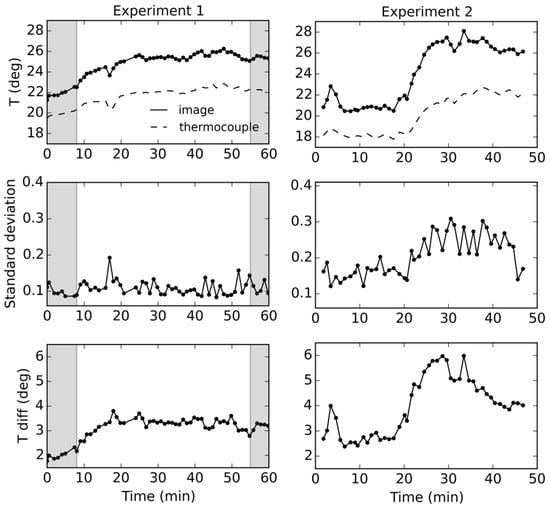
Figure 6.
Retrieved image and thermocouple temperature measurement of the calibration target with corresponding differences between the two and image standard deviations. Shaded areas indicate times at which the additional light sources were turned off.
During Experiment 2, the measurements were much more variable (Figure 6); this was due to changing weather conditions, i.e., moving cloud cover. Occasional periods of sunshine increased the shortwave radiation inside the greenhouse leading to an increase in temperature of the air and surfaces. Consequently, the longwave background radiation emitted by surrounding objects increased (causing differences between the image and thermocouple measurements up to 6 °C). This influence can also be observed in the image standard deviation value of the target, which almost doubled. Otherwise, prior to clouds clearing, the difference between image and thermocouple values remained at the same level as in Experiment 1 (around 2.5 °C, apart from a single spike caused by a brief sunshine period).
As presented, the image readings were significantly affected by the large variations in background radiance emitted from surrounding objects, in particular in Experiment 2. If left unaccounted for, these changes would inhibit temporal analysis of the datasets.
3.3. Thermocouple and Image Measurements of Trees over Time
During Experiment 1, air temperature inside of the greenhouse was stable until the additional light source was turned on. Afterwards, a substantial, yet steady, increase in air temperature from 21 °C to around 24 °C was observed. Thermocouples attached to different parts of the canopies showed different rates of temperature increase (Figure 7). At the beginning of the experiment, all measurements were close together, showing barely any difference in temperature readings. However, with additional radiation, readings started to separate, with higher increases recorded for upper sections of the trees. Throughout Experiment 2, the air temperature varied more as a result of moving cloud cover. Intermittent sunshine caused temperature spikes, whilst partial cloud clearing led to a drastic ambient temperature increase from 20°C to 25 °C. In this experiment, from the beginning, there was a clear difference between the upper and lower parts of the canopies. However, there were no considerable differences between the mildly stressed and the control plant, until after Minute 30, when readings from the canopy top separated. The upper parts of the canopies were located closer to the light source, and consequently were receiving more direct radiation, leading to a steeper increase in the temperature when compared to the lower parts. Within Experiment 1, there were visible differences in temperature readings between the control and stressed canopies, the second being warmer. However, those observations cannot be conclusive, as the differences could have been caused by the distribution of the thermocouples on trees, e.g., placement at uneven distance from the light source. Therefore, the thermocouple measurements were primarily used for validating thermal camera readings and assessing the performance of the normalization for the background radiance.
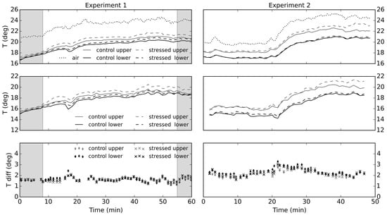
Figure 7.
Temperature readings acquired by the thermocouples (top); and the thermal camera (middle) for the lower and upper parts of tree crowns; and differences between the two (bottom). Experiment 1 involved a moderately, whilst Experiment 2 a mildly stressed tree. Shaded areas indicate times at which the additional light sources were turned off.
The thermocouple measurements were compared to the image readings, extracted from the corresponding regions. The differences between the temperatures recorded by the thermocouples and the camera were calculated (with image temperatures subtracted from the thermocouple measurements), and are shown in Figure 7. In Experiment 1, image temperature extracted for each thermocouple location were on average different by 1.64 °C, which is within the thermocouple accuracy threshold of ±2.2 °C. However, the temperature values acquired for Experiment 2 marginally exceeded the threshold with average difference of 2.26 °C. The image canopy temperature readings were normalized for changes in background radiance levels, which allowed minimization of the temporal variability of measurements. The standard deviation of the offsets from the thermocouple readings was reduced from 0.46 °C to 0.20 °C in Experiment 1 and from 1.00 °C to 0.32 °C in the Experiment 2.
3.4. Vertical Distribution of Canopy Temperature
The temporal and vertical variation in canopy temperature extracted from the imagery, alongside pixel count histograms, for both experiments is shown in Figure 8. For all of the trees, the upper parts of the canopies were considerably warmer than the lower parts. The difference increased as time went by, caused by an input of additional shortwave radiation and consequent warming up of the room. This effect was probably mainly caused by the proximity to the light (and consequently heat) source and limited foliage of the tree top. In canopy parts characterized by very low volume, the temperature was higher, which is particularly evident in the transition from a single tree leader to sections with branches. For example, for the control tree in Experiment 2, the difference amounts to about 4 °C. The higher temperature in the areas of scarce foliage is likely to have been caused by inclusion of mixed pixels, containing readings from both the canopy and background. Despite attempts to exclude all mixed pixels during the masking stage, some may have remained and contributed to higher temperature measurements. Therefore, for comparison between the plants, the low canopy volume mask was applied prior to further analysis.
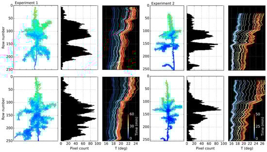
Figure 8.
Vertical distribution of canopy temperature over time, retrieved from thermal imagery, for: stressed plant (top); and control plant (bottom).
For all remaining rows, the temperature differences between the stressed and control plants were computed, as shown in Figure 9. In Experiment 1, the control tree was colder than the stressed tree in most image rows, and this difference was further accentuated over time. The only region where the stressed plant was colder were rows 110–120, most likely an artifact of structural differences; within this region, the stressed plant consists of multiple branches clumped closely together, whilst the control plant has limited foliage. Conversely, in Experiment 2, the temperature differences between the trees seemed to be dictated primarily by structural variances across the canopies, rather than stress; lower temperatures were recorded in rows of high foliage volume, and foliage clumping around the main stem.
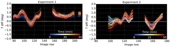
Figure 9.
Temperature difference between stressed and control plants calculated from average derived for each image row.
3.5. Differences in Thermal Response of Control and Stressed Plants
To further explore the thermal response of control and stressed plants over time, average canopy temperature values were calculated for each image. Utilizing the derived low canopy volume mask, mean, median and standard deviation values of the rest of the pixels were computed. The mean and median response over time, alongside the difference in mean temperatures between stressed and control plants for both experiments, are shown in Figure 10.
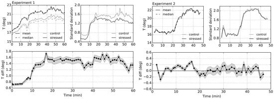
Figure 10.
Mean and median temperature values over time for plants, alongside standard deviation (top); and difference in mean temperatures between stressed and control plants with 99% confidence intervals derived with Welch’s t-test (bottom). If confidence interval overlaps Tdiff = 0 °C, the temperature means are not significantly different at the given confidence level.
In Experiment 1, the mean and median values for the moderately stressed plant were the same, indicating symmetric distribution of temperature values across the canopy. However, for the control tree, the distribution became skewed upon the turning on of lamps (turned on between Minutes 8 and 55): the mean was greater than the median, whilst interquartile range by Minute 20 increased by 0.54 °C (as opposed to 0.45 °C for the stressed plant). This suggests that the canopies responded to the change in environmental conditions in a different manner; the stressed plant warmed up fairly uniformly, whilst the control canopy only showed high levels of temperature change in its upper part. As a result, the overall temperature difference between the trees drastically increased after the additional light source was turned on, i.e., from 0.75 °C to 1.5 °C. This difference started declining again after the lamps were turned off. Nevertheless, the difference in standard deviation over time between the two plants remained at the same level of approximately 0.2 °C, despite the sudden increase (by around 0.8 °C) when the additional light source was turned on. Welch’s t-test showed that the difference between the canopy temperature means was statistically significant throughout the whole experiment, even under low illumination conditions.
Throughout Experiment 2, despite slightly different canopy structure and volume distribution, the mean and median temperature values of the plants were nearly identical. The standard deviation of both plants increased significantly by around 1.1 °C, with greater differences between the upper and lower canopy caused by the occasional periods of sunshine increasing the amount of shortwave radiation and air temperature inside of the greenhouse. However, the mild stress, under which the plant was put, did not exhibit itself in statistically significant differences in canopy temperature; the overall temperature difference between the trees continuously oscillated around 0 °C, notwithstanding drastic environmental change in radiance and ambient temperature.
4. Discussion
The experiments showed that the thermal camera, following calibration and a basic normalization for background radiation, is capable of monitoring temporal temperature change in conifer tree foliage. A significant non-uniformity was found across the camera’s field of view with differences exceeding 2 °C in some cases. In thermography of plants, where differences in temperature are usually small, such non-uniformity, if left unaccounted for, might significantly affect the results when measurements originating from different pixels are compared. For ground-based applications, the relative temperature change within the same pixels may still be investigated, such as in Kim et al. [], providing pixel level sensor responses are linear in terms of emitted flux versus digitized flux over a range of desired temperatures, since the same error in the estimation of absolute temperature would persist. Following the non-uniformity correction, the spatial variation of canopy temperature was well characterized, showing that thermal imagery can provide a reliable means for thermal analysis of conifers. Nevertheless, we were unable to fully determine accuracy of retrieval of absolute canopy temperature values, as the readings for one of the experiments marginally exceeded the typical type K thermocouple accuracy threshold of ±2.2 °C. A high uncertainty was introduced into thermocouple measurements, disallowing absolute validation of the camera readings. Due to foliage type, to avoid causing mechanical damage, the thermocouples were not firmly attached to needles, and instead, they were wrapped inside of needle clumps. It is therefore very likely that the thermocouple measurements were not only affected by the needle surface temperature, but also, to some degree, by the surrounding air. Nevertheless, even though absolute temperature values could not be fully ascertained, the background correction did normalize the camera readings over time. The differences between all thermocouples and image values were relatively stable throughout the experiments (exhibiting standard deviation of temperature offsets of 0.20 °C in Experiment 1 and 0.32 °C in the Experiment 2). The camera effectively monitored the temperature trend over time for all thermocouple locations, and recorded temperature differences between the different locations. The canopy temperature could otherwise be measured using thermo-radiometers. However, these return an aggregation of temperature measurements for an area, the extent of which depends on the view angle and distance from the canopy []; in this study, point measurement was more appropriate for validation of the intra-crown temperature variation.
For a more accurate correction of the background radiation, at least two different calibration targets of known emissivity and surface temperature would have to be utilized. With temperature readings from at least two targets (ideally colder and hotter than the measured object, i.e., plants), radiometric calibration coefficients could be calculated based on a linear regression, which would allow brightness temperature (as measured by the camera) to be related to the actual surface temperature. Initially, we tried utilizing diamond diffusion foil as the second target, which proved infeasible due to strong directional dependence of its emissivity. In a UAV survey setting, the same approach based on an empirical line correction can be used, with at least three contrasting ground targets, whose temperatures are continuously being monitored. Inclusion of a third target not only provides redundancy, but also allows assessment of the quality of fit between recorded and actual temperatures. To retrieve the calibration coefficients, the deployed targets would normally be imaged at the beginning and the end of the survey [], although additional mid-flight calibrations [] may be preferred on longer flights or if weather conditions are rapidly changing. Using the empirical line calibration method, Gomez-Candon et al. [] reported R2 value of 0.768 in linear regression of apple tree canopy temperature measurements from calibrated thermal imagery and from radio-thermometers positioned 1.2 m above top of the tops of the canopies. Alternatively, surface temperatures may be obtained using radiative transfer equation, such as MODTRAN [], as demonstrated by Berni et al. [] who observed reduction in RMSE of target temperature measurements from 3.44 K to 0.89 K following the correction.
Spatio-temporal analysis of the imagery provided an insight into thermal properties of the plants. In canopy parts characterized by very low volume the temperature was considerably higher. The higher temperature in the areas of scarce foliage is likely to have been caused by inclusion of mixed pixels, containing readings from both the canopy and background. Those areas could also potentially have closed stomata as a result of increased insolation and transpiration, leading to an increase in temperature. Potentially, larger influence of trunk pixels on the retrieved mean temperature was also a contributor; Kim et al. [] showed there is a consistent difference between leaves and trunks in ponderosa pines, especially during the afternoon, with the latter being warmer. After exclusion of the areas with minimal foliage, very mild stress did not exhibit itself, despite drastic changes in ambient temperature and radiance levels; the temperature readings for both the stressed and control plant were closely related throughout the whole test (Experiment 2). However, with higher stress levels (Experiment 1), there was a clear distinction between the two plants, which then doubled after the additional light source was turned on. The observed increase in temperature as a response to plant water stress is in accordance with many previous studies [,,]. Nevertheless, further work on coniferous trees using nadir viewing imagery acquired under field conditions would be required to fully assess the feasibility of using UAV-borne thermal imagery within forest environments.
The standard deviation of the crown temperature was suggested to be an indicator of stress by some [,]. Fuchs [], on a simulated cotton canopy, demonstrated that water stress, apart from increasing crown temperature, widens the range of temperature variation within the canopy. This is due to leaf orientation playing a great role in the energy budget, especially when stomata are closed. In more stressed canopies greater variation in temperatures may be detected due to the change in leaf angle resulting from wilting. Gonzalez-Dugo et al. [] observed that the variability of canopy temperature increased during the early stages of water stress, and diminished when the stress became more severe. No such trend was observed within this study; with mild stress, there was no difference between the trees, whilst with the onset of moderate stress, the control plant exhibited minimally higher intra-crown temperature variability. This indicator seems not to be applicable to mildly or moderately stressed conifers; as it is attributed to the change in leaf orientation upon onset of stress, the effect would be none or very minimal. However, it might prove feasible for coniferous trees undergoing extreme levels of stress. In grapevines, the intra-crown variations in temperature were not impacted by water status either, a supposed effect of the non-random distribution of leaf angles in the canopies [,]. An additional limitation of this indicator is that the variation in canopy temperature is also affected by external conditions. In both experiments shown here, the standard deviation of canopy temperature exhibited a steep increase upon an increase in shortwave radiation level, suggesting this indicator could only allow for a relative comparison between trees investigated under same conditions. Gonzalez-Dugo et al. [] also recognized that the intra-crown temperature variability cannot be clearly compared without taking absolute canopy temperature into account.
The variations in canopy temperature are highly dependent on environmental factors. In a ponderosa pine forest, the thermal dynamics were shown to be mainly controlled by air temperature, water vapor and radiation []. Here, similarly, the increase in canopy temperature was dictated by the increased radiation levels and ambient temperature. It was also observed that the plants warmed up in different manners—the moderately stressed plant fairly uniformly, whilst the control canopy exhibited lower levels of temperature change in its lower canopy. From the physiological point of view, the increase in temperature difference between the two trees would be caused by the different response of the plants to the additional radiation. A stressed plant would have its stomata closed to prevent the loss of water through transpiration, also preventing the entry of carbon dioxide into the leaves and disrupting the photosynthesis []. This could explain the observed fairly uniform increase in temperature across the canopy, appearing to be mostly dependent on the change in ambient temperature. In contrast, with random distribution of foliage in a control canopy, the leaf response may vary depending on their shade history—some leaves upon illumination will have their stomata open, others after some time of illumination may still keep their stomata closed [,]. Nevertheless, even under low light conditions, there was a clear distinction in canopy temperature between the control and the moderately stressed tree, showing potential of low-cost thermography for investigating stress in conifers. As the differences between stressed and control plants were greatest when the amount of illumination and air temperature increased, it is deduced UAV-borne thermal surveys investigating tree stress should be performed at the time of maximum evaporative demand. Maximum evaporative demand is normally expected to occur in the early afternoon [], when air temperatures driven by radiation peak. However, other environmental factors, such as humidity or wind speed, have also been shown to also affect the evaporative demand, and consequently temperature at a canopy level []. The question remains how they may influence the ability to distinguish stressed plants, in particular in countries with moderate air temperatures year-round, such as Scotland.
The approach shown in here of direct investigation of canopy temperature can only be applied in a relative mode, comparing plants imaged under exactly the same conditions (in practice that means plants located within the same image). This is due to leaf and canopy temperature being dependent on air temperature, humidity, wind speed and absorbed net radiation []. Thermal stress indices have been most commonly used to overcome this problem, normalizing the results for environmental variation, and allowing for multi-spatial and/or multi-temporal comparison. The most commonly used stress indices include the CTD (shown to be adversely affected by weather conditions []), CWSI and Ig. CWSI and Ig were shown to not be influenced by the amount of incoming shortwave radiation and vapor pressure deficit; however, they are affected by air temperature and wind speed []. Optimal conditions, based on modeled discriminative power, for application of those indices include high air temperature, incoming shortwave radiation and vapor pressure deficit and low wind speed [].
5. Conclusions
With the development of UAVs, high spatial resolution data have become more accessible than ever before. Furthermore, UAVs can help in bridging the gap between ground surveys and other more traditional remote sensing platforms. However, their main constraint is the limited payload they offer, requiring the use of miniature sensors. In the thermal domain, miniaturized uncooled sensors would normally have to be used, which have slower response times and are less sensitive than cooled detectors. This study investigated whether a low-cost miniature thermal camera, destined to be used on a UAV platform, is capable of providing reliable canopy temperature measurements of conifers. Following camera calibration and a basic normalization for background radiation, both the spatial and temporal variation of canopy temperature was well reflected. Furthermore, there was a clear distinction in canopy temperature between the investigated control and the moderately stressed tree, showing the potential of low-cost thermography for investigating stress in conifers. However, a change in environmental conditions altered the magnitude of this difference, i.e., rising radiation level and ambient temperature led to an increase in the difference between the average canopy temperatures. The performance of thermography when applied to conifer stress investigation may therefore depend on environmental conditions under which the data are acquired. Research in a fully controlled environment could quantify the influence of different environmental factors, and define conditions under which thermal imagery can be used most effectively in different climates. Such guidance might help with planning UAV-borne campaigns utilizing low-cost sensors by identification of best acquisition times, when temperature differences between plants are expected to be greatest.
Acknowledgments
The authors want to thank Chris MacLellan from the University of Edinburgh and Georgios Xenakis from Forest Research for their help. This work was supported by the Natural Environment Research Council (NERC) studentship award (reference number: 1368552). The thermal camera was purchased through Royal Society Research Grant RG130211. Access to specialist equipment was provided by the NERC Field Spectroscopy Facility loan (710.114) through NERC airborne grant (GB 14-04). The costs of open access publication were covered by NERC. We would also like to thank the anonymous reviewers for their constructive comments which have helped improve the manuscript.
Author Contributions
Magdalena Smigaj performed the laboratory measurements—camera calibration and FTIR measurements. Magdalena Smigaj and Juan C. Suarez conceived, designed and performed the tree experiments. Magdalena Smigaj processed the data, analyzed the results and drafted the manuscript with technical guidance from Rachel Gaulton. Rachel Gaulton, Juan C. Suarez, and Stuart L. Barr contributed to the editing of this paper, providing insightful comments and suggestions. All authors have read and approved the final manuscript.
Conflicts of Interest
The authors declare no conflict of interest.
References
- Ray, D.; Morison, J.; Broadmeadow, M. Climate Change: Impacts and Adaptation in England’s Woodlands. 2010. Available online: https://www.forestry.gov.uk/fr/climatechangeengland (accessed on 31 July 2017).
- Taub, D. Effects of Rising Atmospheric Concentrations of Carbon Dioxide on Plants. Available online: http://www.nature.com/scitable/knowledge/library/effects-of-rising-atmospheric-concentrations-of-carbon-13254108 (accessed on 31 July 2017).
- Christensen, J.H.; Christensen, O.B. A summary of the prudence model projections of changes in European climate by the end of this century. Clim. Chang. 2007, 81, 7–30. [Google Scholar] [CrossRef]
- Déqué, M.; Rowell, D.P.; Lüthi, D.; Giorgi, F.; Christensen, J.H.; Rockel, B.; Jacob, D.; Kjellström, E.; de Castro, M.; van den Hurk, B. An intercomparison of regional climate simulations for Europe: Assessing uncertainties in model projections. Clim. Chang. 2007, 81, 53–70. [Google Scholar] [CrossRef]
- Blenkinsop, S.; Fowler, H.J. Changes in European drought characteristics projected by the prudence regional climate models. Int. J. Climatol. 2007, 27, 1595–1610. [Google Scholar] [CrossRef]
- Murphy, J.M.; Sexton, D.M.H.; Jenkins, G.J.; Boorman, P.M.; Booth, B.B.B.; Brown, C.C.; Clark, R.T.; Collins, M.; Harris, G.R.; Kendon, E.J.; et al. UK Climate Projections Science Report: Climate Change Projections; Met Office Hadley Centre: Exeter, UK, 2009.
- Madsen, H.; Lawrence, D.; Lang, M.; Martinkova, M.; Kjeldsen, T.R. Review of trend analysis and climate change projections of extreme precipitation and floods in Europe. J. Hydrol. 2014, 519, 3634–3650. [Google Scholar] [CrossRef]
- Lehner, B.; Döll, P.; Alcamo, J.; Henrichs, T.; Kaspar, F. Estimating the impact of global change on flood and drought risks in Europe: A continental, integrated analysis. Clim. Chang. 2006, 75, 273–299. [Google Scholar] [CrossRef]
- Tudoran, M.-M.; Marquer, L.; Jönsson, A.M. Historical experience (1850–1950 and 1961–2014) of insect species responsible for forest damage in Sweden: Influence of climate and land management changes. For. Ecol. Manag. 2016, 381, 347–359. [Google Scholar] [CrossRef]
- Raffa, K.F.; Aukema, B.H.; Bentz, B.J.; Carroll, A.L.; Hicke, J.A.; Turner, M.G.; Romme, W.H. Cross-scale drivers of natural disturbances prone to anthropogenic amplification: The dynamics of bark beetle eruptions. BioScience 2008, 58, 501–517. [Google Scholar] [CrossRef]
- Hubbart, J.A.; Guyette, R.; Muzika, R.-M. More than drought: Precipitation variance, excessive wetness, pathogens and the future of the western edge of the eastern deciduous forest. Sci. Total Environ. 2016, 566, 463–467. [Google Scholar] [CrossRef] [PubMed]
- González-Dugo, M.P.; Moran, M.S.; Mateos, L.; Bryant, R. Canopy temperature variability as an indicator of crop water stress severity. Irrig. Sci. 2006, 24, 233–240. [Google Scholar] [CrossRef]
- Jones, H.G. Use of infrared thermometry for estimation of stomatal conductance as a possible aid to irrigation scheduling. Agric. For. Meteorol. 1999, 95, 139–149. [Google Scholar] [CrossRef]
- Chaerle, L.; Caeneghem, W.V.; Messens, E.; Lambers, H.; Van Montagu, M.; Van Der Straeten, D. Presymptomatic visualization of plant-virus interactions by thermography. Nat Biotechnol 1999, 17, 813–816. [Google Scholar] [PubMed]
- Lindenthal, M.; Steiner, U.; Dehne, H.W.; Oerke, E.C. Effect of downy mildew development on transpiration of cucumber leaves visualized by digital infrared thermography. Phytopathology 2005, 95, 233–240. [Google Scholar] [CrossRef] [PubMed]
- Jackson, R.D.; Idso, S.B.; Reginato, R.J.; Pinter, P.J. Canopy temperature as a crop water stress indicator. Water Resour. Res. 1981, 17, 1133–1138. [Google Scholar] [CrossRef]
- Leinonen, I.; Grant, O.M.; Tagliavia, C.P.P.; Chaves, M.M.; Jones, H.G. Estimating stomatal conductance with thermal imagery. Plant Cell Environ. 2006, 29, 1508–1518. [Google Scholar] [CrossRef] [PubMed]
- Idso, S.B.; Jackson, R.D.; Pinter, P.J., Jr.; Reginato, R.J.; Hatfield, J.L. Normalizing the stress-degree-day parameter for environmental variability. Agric. Meteorol. 1981, 24, 45–55. [Google Scholar] [CrossRef]
- Keener, M.E.; Kircher, P.L. The use of canopy temperature as an indicator of drought stress in humid regions. Agric. Meteorol. 1983, 28, 339–349. [Google Scholar] [CrossRef]
- Maes, W.H.; Steppe, K. Estimating evapotranspiration and drought stress with ground-based thermal remote sensing in agriculture: A review. J. Exp. Bot. 2012, 63, 4671–4712. [Google Scholar] [CrossRef] [PubMed]
- Alderfasi, A.A.; Nielsen, D.C. Use of crop water stress index for monitoring water status and scheduling irrigation in wheat. Agric. Water Manag. 2001, 47, 69–75. [Google Scholar] [CrossRef]
- Erdem, Y.; Arin, L.; Erdem, T.; Polat, S.; Deveci, M.; Okursoy, H.; Gültaş, H.T. Crop water stress index for assessing irrigation scheduling of drip irrigated broccoli (brassica oleracea l. Var. Italica). Agric. Water Manag. 2010, 98, 148–156. [Google Scholar] [CrossRef]
- Taghvaeian, S.; Comas, L.; DeJonge, K.C.; Trout, T.J. Conventional and simplified canopy temperature indices predict water stress in sunflower. Agric. Water Manag. 2014, 144, 69–80. [Google Scholar] [CrossRef]
- Gonzalez-Dugo, V.; Zarco-Tejada, P.; Berni, J.A.J.; Suárez, L.; Goldhamer, D.; Fereres, E. Almond tree canopy temperature reveals intra-crown variability that is water stress-dependent. Agric. For. Meteorol. 2012, 154–155, 156–165. [Google Scholar] [CrossRef]
- Berni, J.A.J.; Zarco-Tejada, P.J.; Sepulcre-Cantó, G.; Fereres, E.; Villalobos, F. Mapping canopy conductance and CWSI in olive orchards using high resolution thermal remote sensing imagery. Remote Sens. Environ. 2009, 113, 2380–2388. [Google Scholar] [CrossRef]
- Ballester, C.; Jiménez-Bello, M.A.; Castel, J.R.; Intrigliolo, D.S. Usefulness of thermography for plant water stress detection in citrus and persimmon trees. Agric. For. Meteorol. 2013, 168, 120–129. [Google Scholar] [CrossRef]
- Scherrer, D.; Bader, M.K.F.; Korner, C. Drought-sensitivity ranking of deciduous tree species based on thermal imaging of forest canopies. Agric. For. Meteorol. 2011, 151, 1632–1640. [Google Scholar] [CrossRef]
- Seidel, H.; Schunk, C.; Matiu, M.; Menzel, A. Diverging drought resistance of scots pine provenances revealed by infrared thermography. Front. Plant Sci. 2016, 7, 1274. [Google Scholar] [CrossRef] [PubMed]
- Grant, O.M.; Tronina, L.; Ramalho, J.C.; Besson, C.K.; Lobo-Do-Vale, R.; Pereira, J.S.; Jones, H.G.; Chaves, M.M. The impact of drought on leaf physiology of quercus suber l. Trees: Comparison of an extreme drought event with chronic rainfall reduction. J. Exp. Bot. 2010, 61, 4361–4371. [Google Scholar] [CrossRef] [PubMed]
- Mildrexler, D.; Yang, Z.Q.; Cohen, W.B.; Bell, D.M. A forest vulnerability index based on drought and high temperatures. Remote Sens. Environ. 2016, 173, 314–325. [Google Scholar] [CrossRef]
- Kim, Y.; Still, C.J.; Hanson, C.V.; Kwon, H.; Greer, B.T.; Law, B.E. Canopy skin temperature variations in relation to climate, soil temperature, and carbon flux at a ponderosa pine forest in central Oregon. Agric. For. Meteorol. 2016, 226, 161–173. [Google Scholar] [CrossRef]
- Smigaj, M.; Gaulton, R.; Barr, S.L.; Suárez, J.C. UAV-borne thermal imaging for forest health monitoring: Detection of disease-induced canopy temperature increase. Int. Arch. Photogramm. Remote Sens. Spatial Inf. Sci. 2015, XL-3/W3, 349–354. [Google Scholar] [CrossRef]
- Holst, G.C. CCD Arrays, Cameras, and Displays; SPIE Optical Engineering Press: Bellingham, WA, USA, 1998. [Google Scholar]
- Thomas, P.J.; Sinclair, P.; Savachenko, A.; Goldman, P.; Elinas, P.; Pope, T. Signal calibration and stability in an uncooled integrated bolometer array. In Proceedings of the IEEE Aerospace Conference, Snowmass at Aspen, CO, USA, 7 March 1999; pp. 401–409. [Google Scholar]
- Wolf, A.; Pezoa, J.E.; Figueroa, M. Modeling and compensating temperature-dependent non-uniformity noise in IR microbolometer cameras. Sensors 2016, 16. [Google Scholar] [CrossRef] [PubMed]
- Grgic, G.; Pusnik, I. Analysis of thermal imagers. Int. J. Thermophys. 2011, 32, 237–247. [Google Scholar] [CrossRef]
- Nugent, P.W.; Shaw, J.A.; Pust, N.J. Correcting for focal-plane-array temperature dependence in microbolometer infrared cameras lacking thermal stabilization. Opt Eng 2013, 52. [Google Scholar] [CrossRef]
- Hook, S.J.; Abbott, E.A.; Grove, C.; Kahle, A.B.; Palluconi, F. Multispectral thermal infrared data in geological studies. In Manual of Remote Sensing, Remote Sensing for the Earth Sciences; Ryerson, R.A., Rencz, A.N., Eds.; John Wiley & Sons, Inc.: New York, NY, USA, 1999; Volume 3, pp. 59–110. [Google Scholar]
- Jones, H.G. Application of thermal imaging and infrared sensing in plant physiology and ecophysiology. Adv. Bot. Res. 2004, 41, 107–163. [Google Scholar]
- Hecker, C.A.; Smith, T.E.L.; Luz, B.R.; Wooster, M.J. Thermal infrared spectroscopy in the laboratory and field in support of land surface remote sensing. In Thermal Infrared Remote Sensing: Sensors, Methods, Applications; Kuenzer, C., Dech, S., Eds.; Springer: Dordrecht, The Netherlands, 2013; pp. 43–67. [Google Scholar]
- Kaiser, J.F. Digital filters. In System Analysis by Digital Computer; Kuo, F.F., Kaiser, J.F., Eds.; John Wiley and Sons: New York, NY, USA, 1966; pp. 218–285. [Google Scholar]
- Welch, B.L. The significance of the difference between two means when the population variances are unequal. Biometrika 1938, 29, 350–362. [Google Scholar] [CrossRef]
- Gomez-Candon, D.; Virlet, N.; Labbe, S.; Jolivot, A.; Regnard, J.L. Field phenotyping of water stress at tree scale by UAV-sensed imagery: New insights for thermal acquisition and calibration. Precis. Agric. 2016, 17, 786–800. [Google Scholar] [CrossRef]
- Santesteban, L.G.; Di Gennaro, S.F.; Herrero-Langreo, A.; Miranda, C.; Royo, J.B.; Matese, A. High-resolution UAV-based thermal imaging to estimate the instantaneous and seasonal variability of plant water status within a vineyard. Agric. Water Manag. 2017, 183, 49–59. [Google Scholar] [CrossRef]
- Berk, A.; Anderson, G.P.; Bernstein, L.S.; Acharya, P.K.; Dothe, H.; Matthew, M.W.; Adler-Golden, S.M.; Chetwynd, J.H.; Richtsmeier, S.C.; Pukall, B.; et al. MODTRAN4 radiative transfer modeling for atmospheric correction. In Optical Spectroscopic Techniques and Instrumentation for Atmospheric and Space Research III, Proceedings of SPIE’S International Symposium on Optical Science, Engineering, and Instrumentation, Denver, CO, USA, 18–23 July 1999; Larar, A.M., Ed.; SPIE: Washington, DC, USA, 1999; pp. 348–353. [Google Scholar]
- Berni, J.A.J.; Zarco-Tejada, P.J.; Suarez, L.; Fereres, E. Thermal and narrowband multispectral remote sensing for vegetation monitoring from an unmanned aerial vehicle. IEEE Trans. Geosci. Remote Sens. 2009, 47, 722–738. [Google Scholar] [CrossRef]
- Fuchs, M. Infrared measurement of canopy temperature and detection of plant water-stress. Theor. Appl. Climatol. 1990, 42, 253–261. [Google Scholar] [CrossRef]
- Grant, O.M.; Tronina, L.; Jones, H.G.; Chaves, M.M. Exploring thermal imaging variables for the detection of stress responses in grapevine under different irrigation regimes. J. Exp. Bot. 2007, 58, 815–825. [Google Scholar] [CrossRef] [PubMed]
- Moller, M.; Alchanatis, V.; Cohen, Y.; Meron, M.; Tsipris, J.; Naor, A.; Ostrovsky, V.; Sprintsin, M.; Cohen, S. Use of thermal and visible imagery for estimating crop water status of irrigated grapevine. J. Exp. Bot. 2007, 58, 827–838. [Google Scholar] [CrossRef] [PubMed]
- Fereres, E.; Goldhamer, D.A.; Parsons, L.R. Irrigation water management of horticultural crops. Hortscience 2003, 38, 1036–1042. [Google Scholar]
- Phillips, N.; Nagchaudhuri, A.; Oren, R.; Katul, G. Time constant for water transport in loblolly pine trees estimated from time series of evaporative demand and stem sapflow. Trees-Struct. Funct. 1997, 11, 412–419. [Google Scholar] [CrossRef]
- Jones, H.G.; Schofield, P. Thermal and other remote sensing of plant stress. Gen. Appl. Plant Physiol. 2008, 34, 19–34. [Google Scholar]
© 2017 by the authors. Licensee MDPI, Basel, Switzerland. This article is an open access article distributed under the terms and conditions of the Creative Commons Attribution (CC BY) license (http://creativecommons.org/licenses/by/4.0/).