Integration of Information Theory, K-Means Cluster Analysis and the Logistic Regression Model for Landslide Susceptibility Mapping in the Three Gorges Area, China


Abstract
:
1. Introduction
2. Methodology
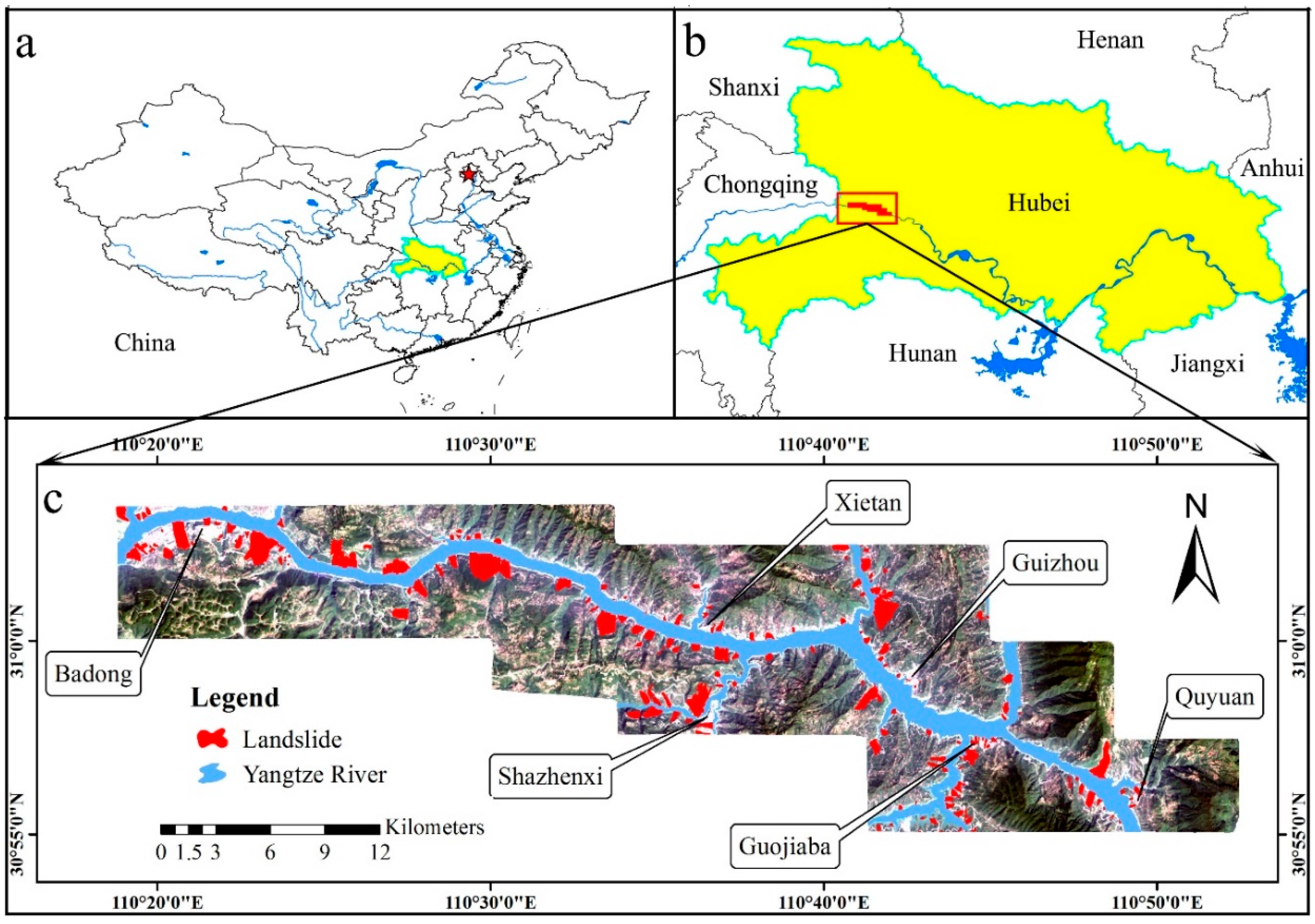
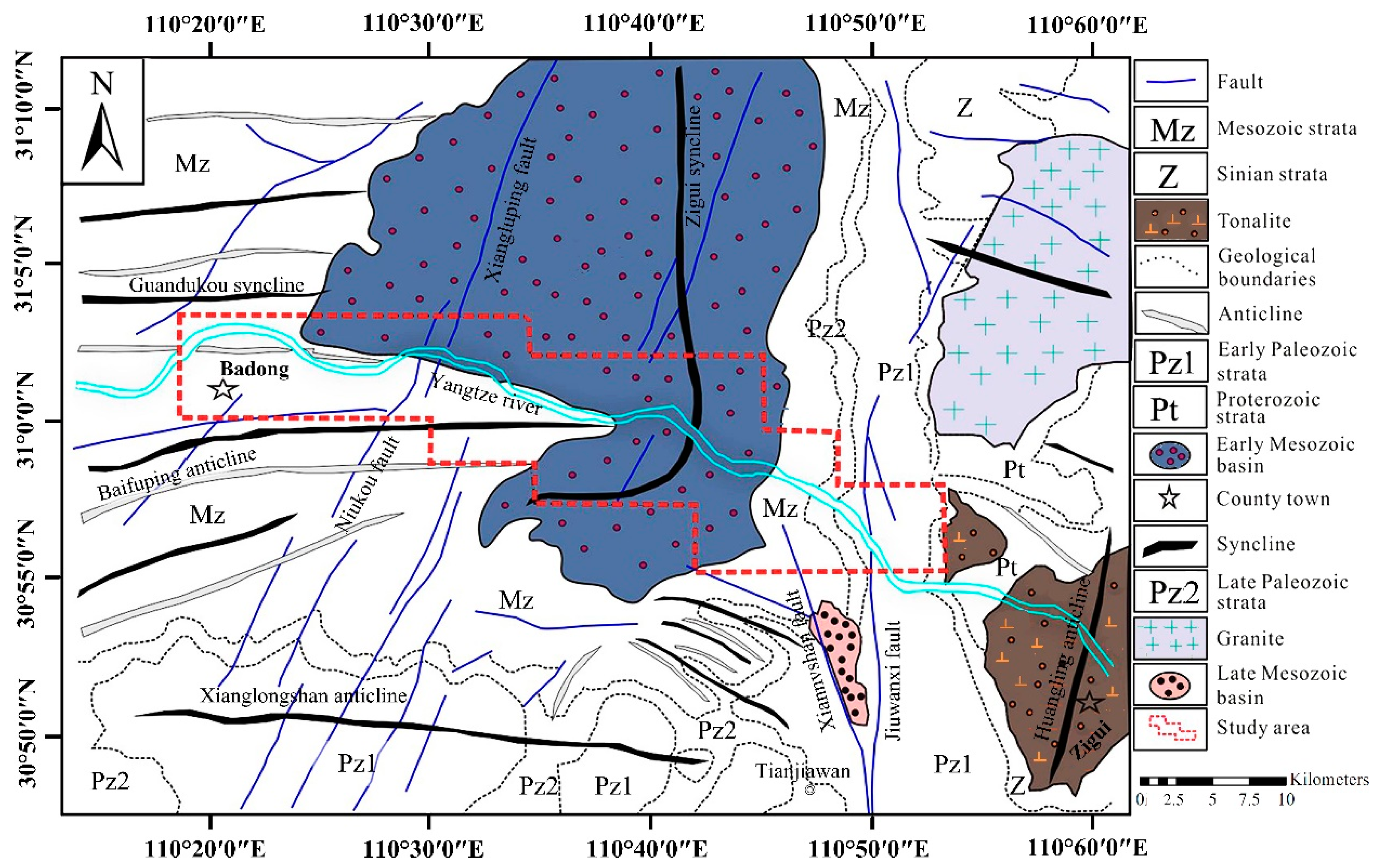
2.1. Study Area
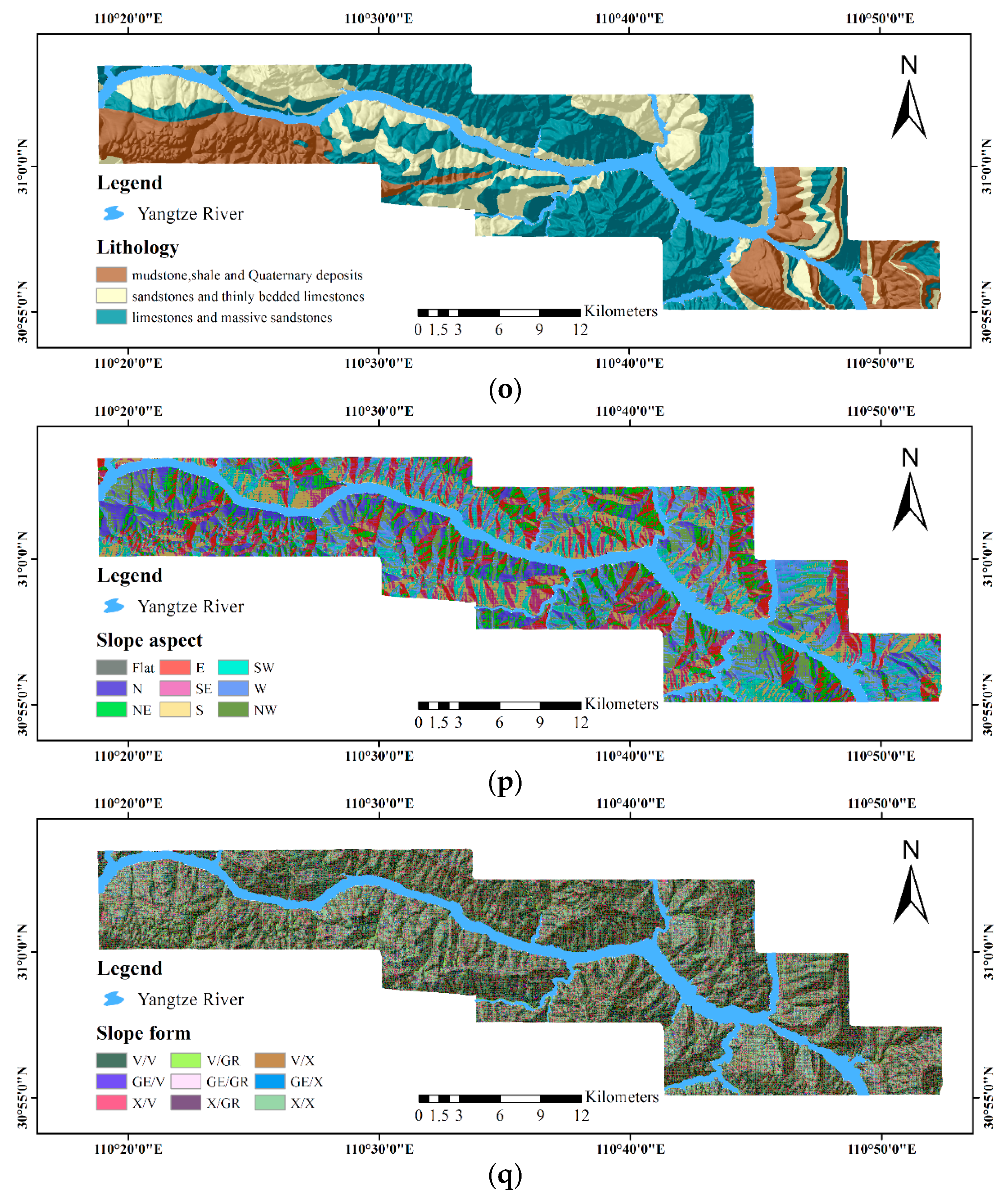
2.1.1. General Characteristics and Geological Setting
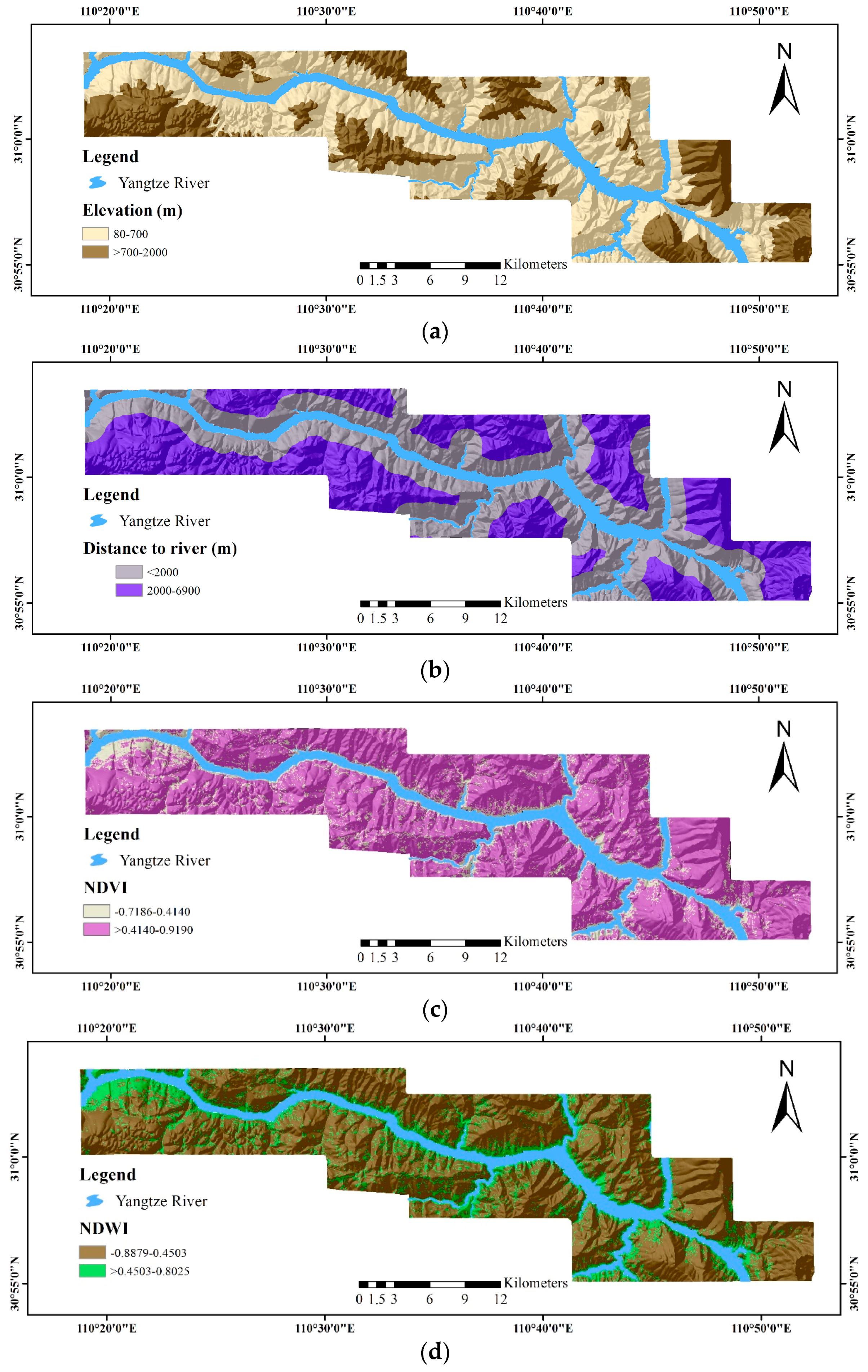
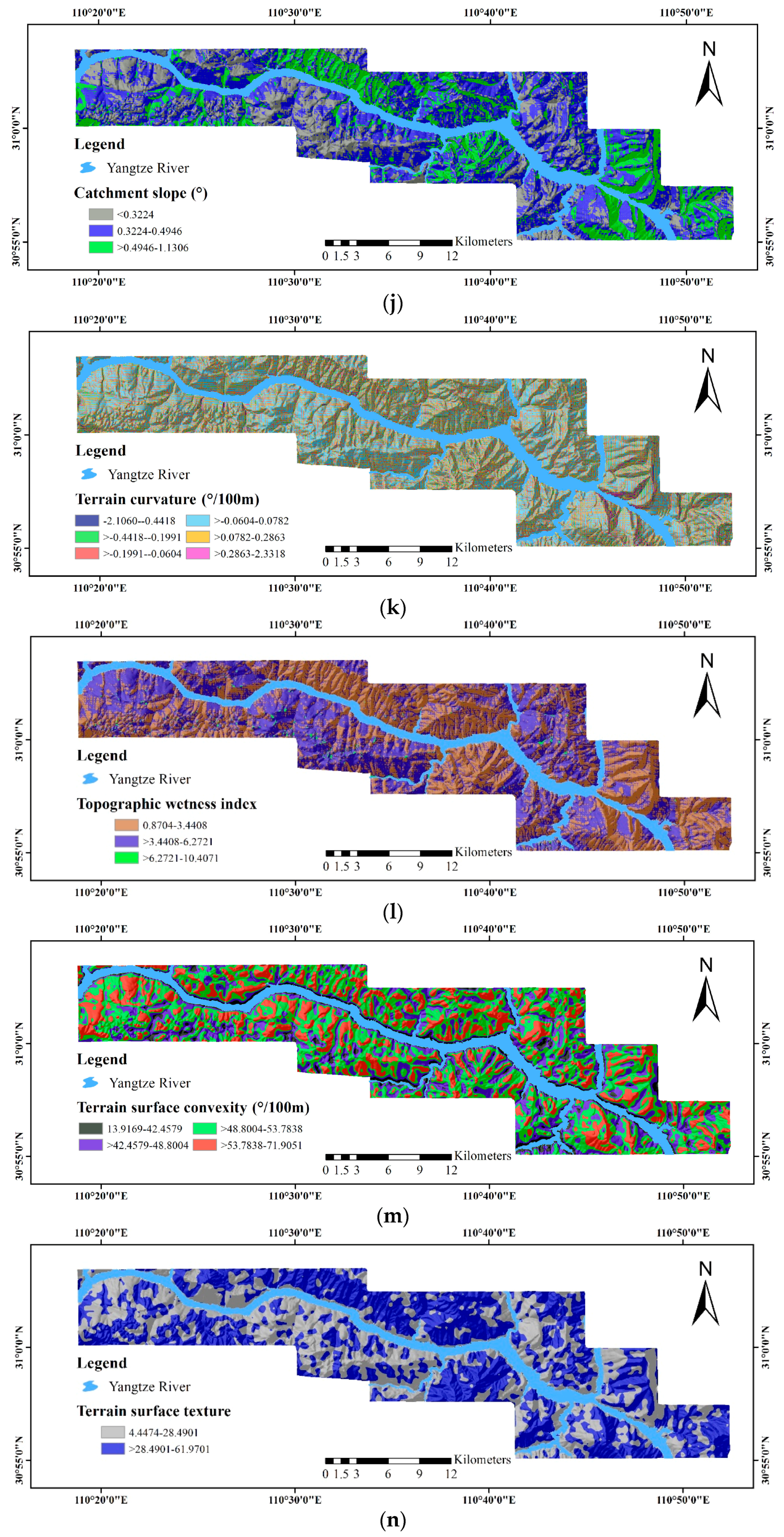
2.1.2. Slope Failures and Causative Factors
- √
- A Landsat-8 OLI image obtained on 14 April 2015, with the path/row number of 125/38. To perform feature extraction, we have performed a series of operations on this multispectral image. This process includes radiometric correction to avoid radiometric errors or distortions over the whole image, geometric correction to avoid geometric distortion due to Earth’s rotation and other imaging conditions from the image and atmospheric correction to remove the effects of the atmosphere on the reflectance values of the image. Meanwhile, Bands 4 and 5 of the image are used for computing the normalized difference vegetable index (NDVI), whereas Bands 3 and 6 of the image are used for computing the normalized difference water index (NDWI).
- √
- The 1:50,000-scale geological maps provided by Hubei Geological Bureau for the exaction of geological factors, including lithology and distance to fault.
- √
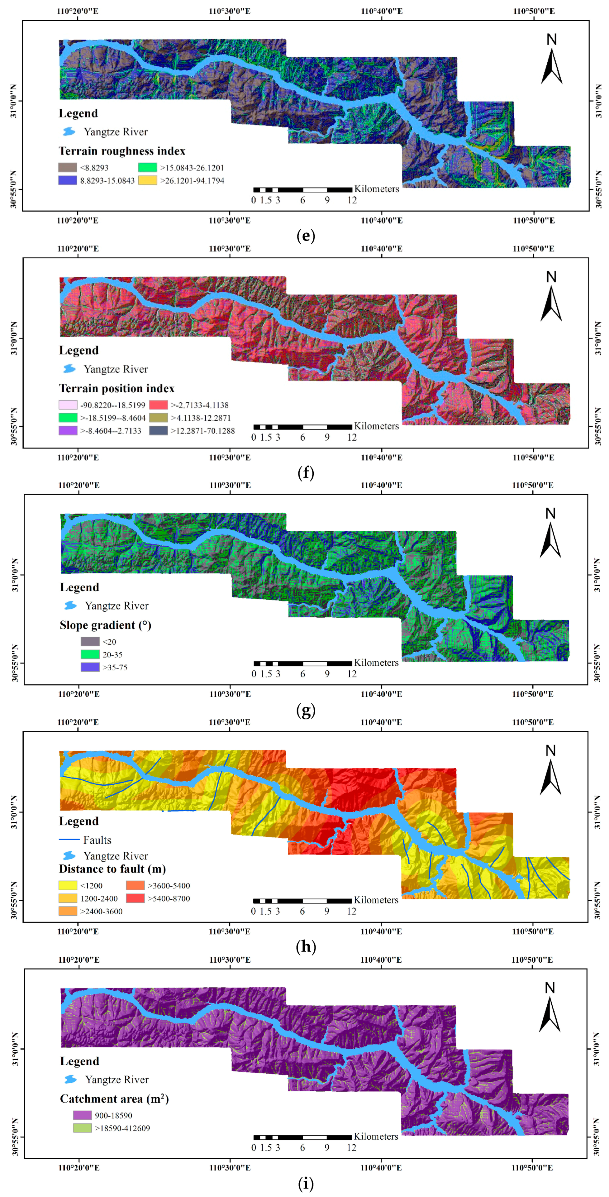
- ASTER GDEM Version 2 (V2) data, representing the surface in raster format, for the extraction of geomorphological and hydrological factors, including elevation, distance to rivers, the terrain roughness index (TRI), the terrain position index (TPI), slope gradient, catchment area, catchment slope, terrain curvature, the topographic wetness index (TWI), terrain surface convexity, terrain surface texture, slope aspect and slope form.
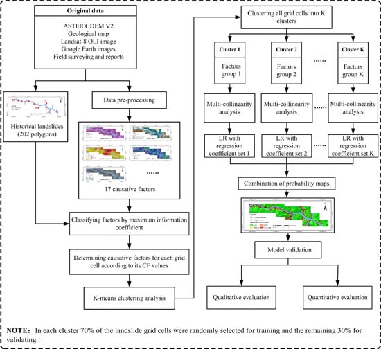
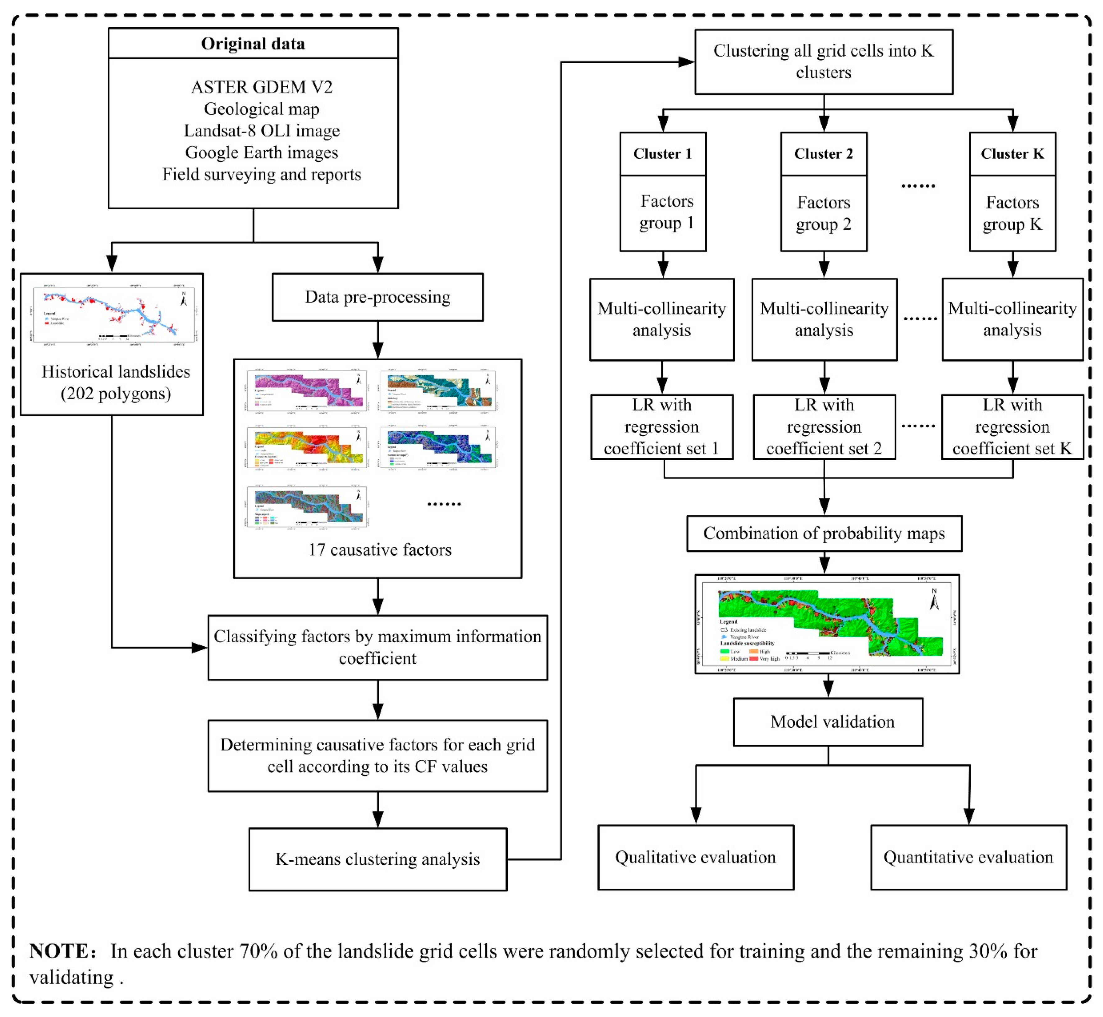
2.2. The Proposed Framework
2.2.1. Information Coefficient Based on Shannon’s Entropy Index
2.2.2. Certainty Factor
2.2.3. K-means Clustering Analysis
2.2.4. Multicollinearity Analysis
2.2.5. Logistic Regression
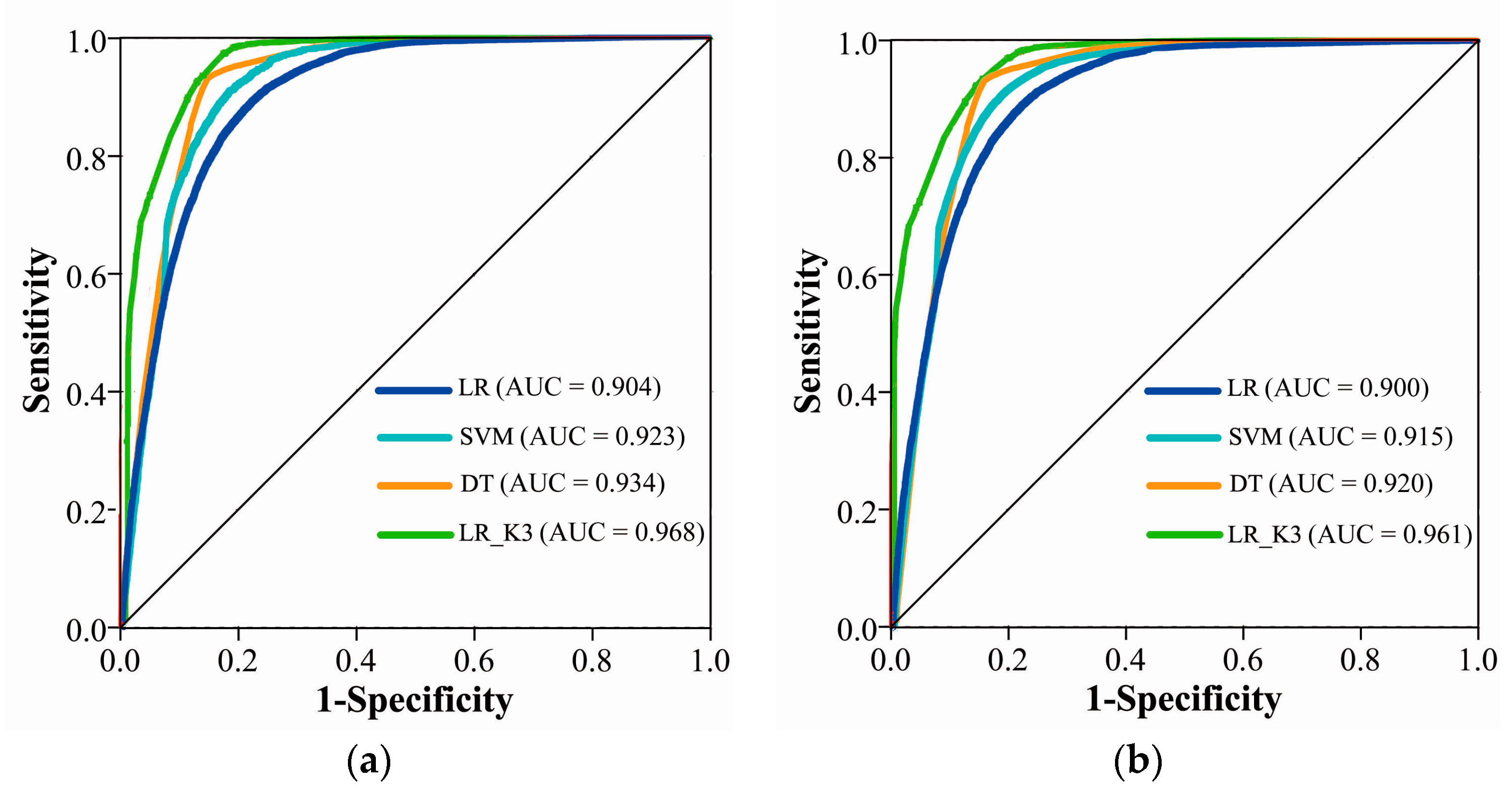
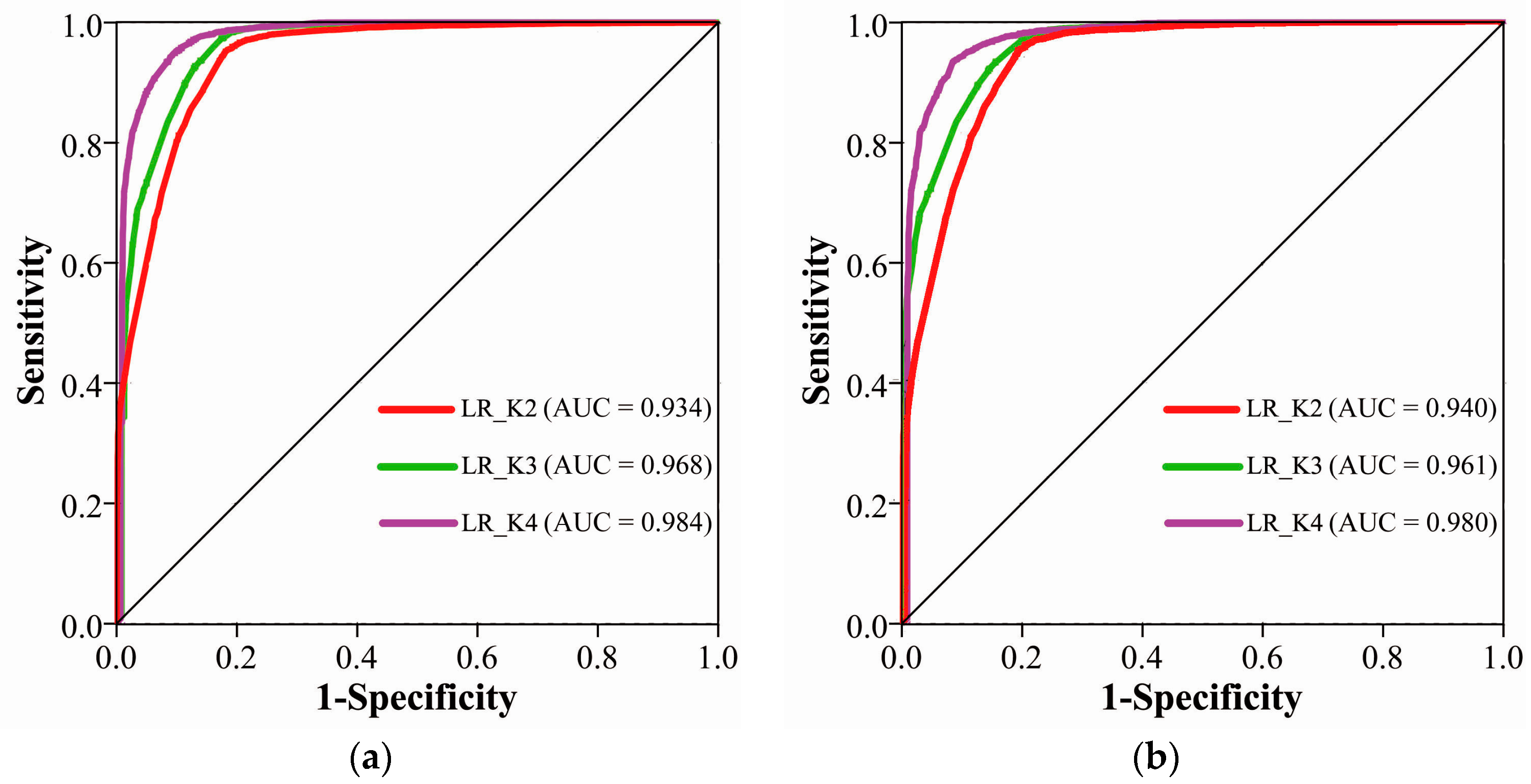
2.3. Objective Evaluation Measures
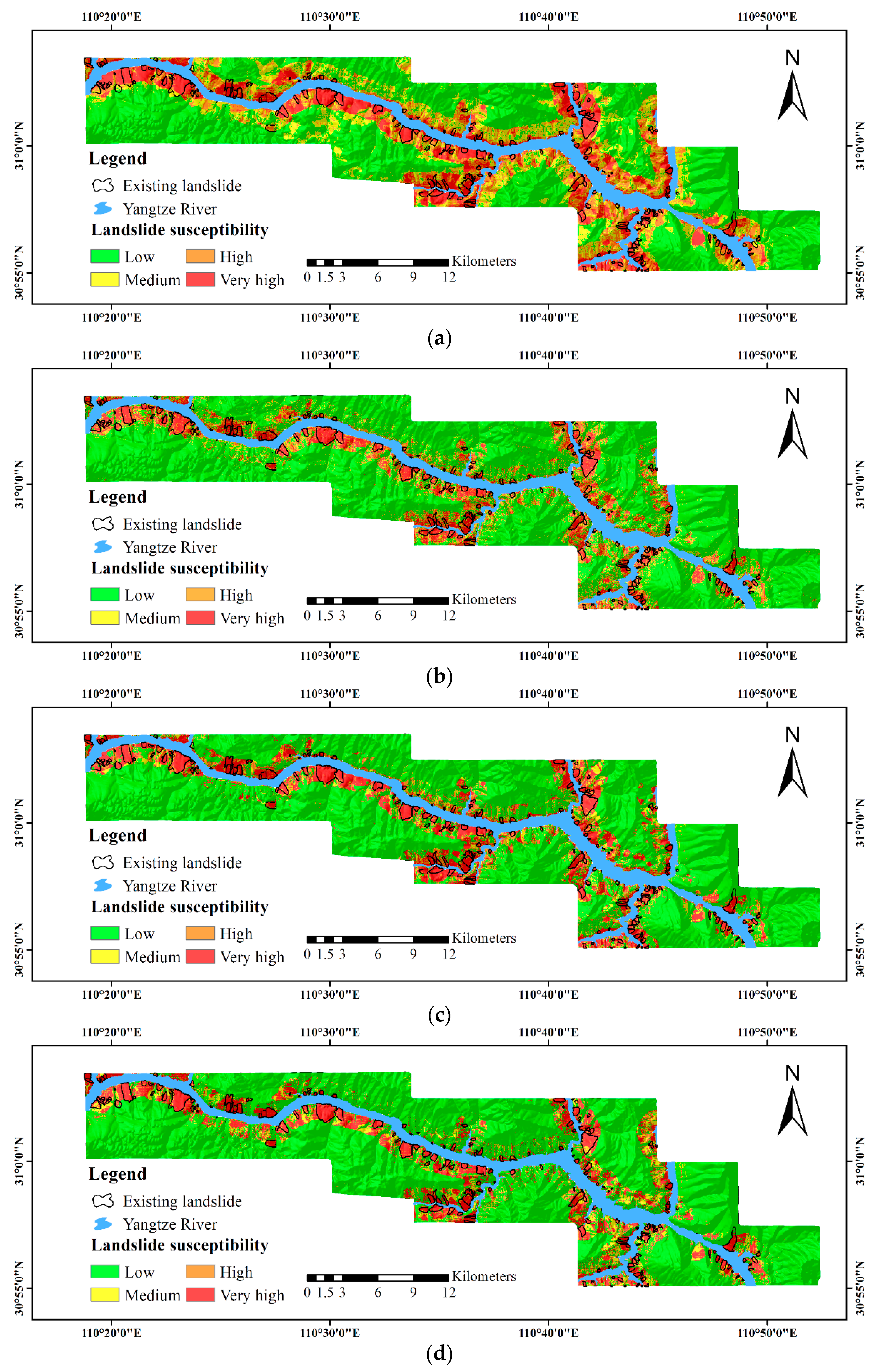
3. Results
3.1. The Construction of the Proposed Framework
3.1.1. Choosing the Number of Classes for Each Causative Factor
3.1.2. Selecting Causative Factors for Each Grid Cell
3.1.3. Clustering Grid Cells into Different Groups
3.1.4. Multicollinearity Analysis of the Selected Causative Factors
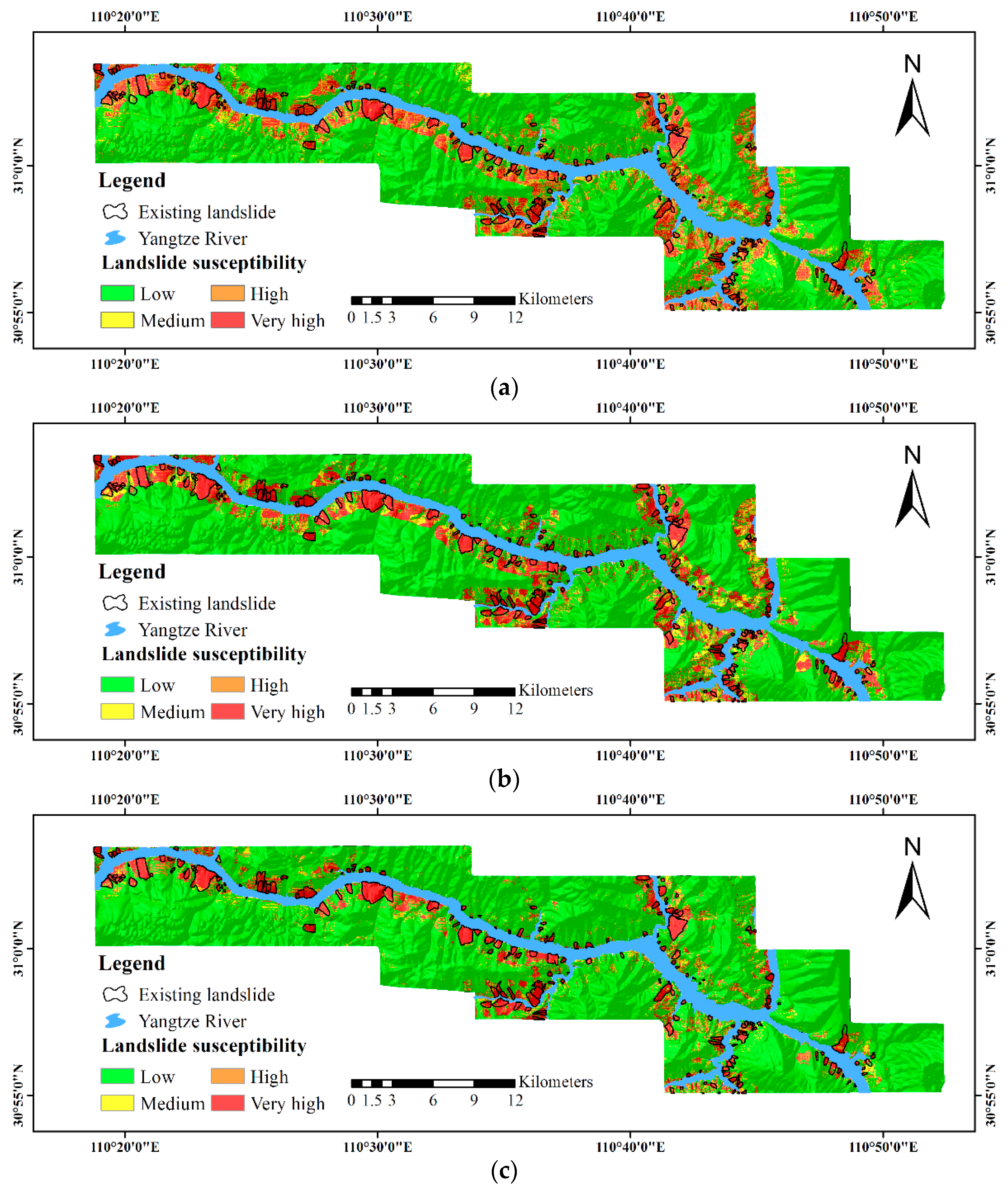
3.2. Validation and Comparison
4. Discussion
4.1. Impact of K
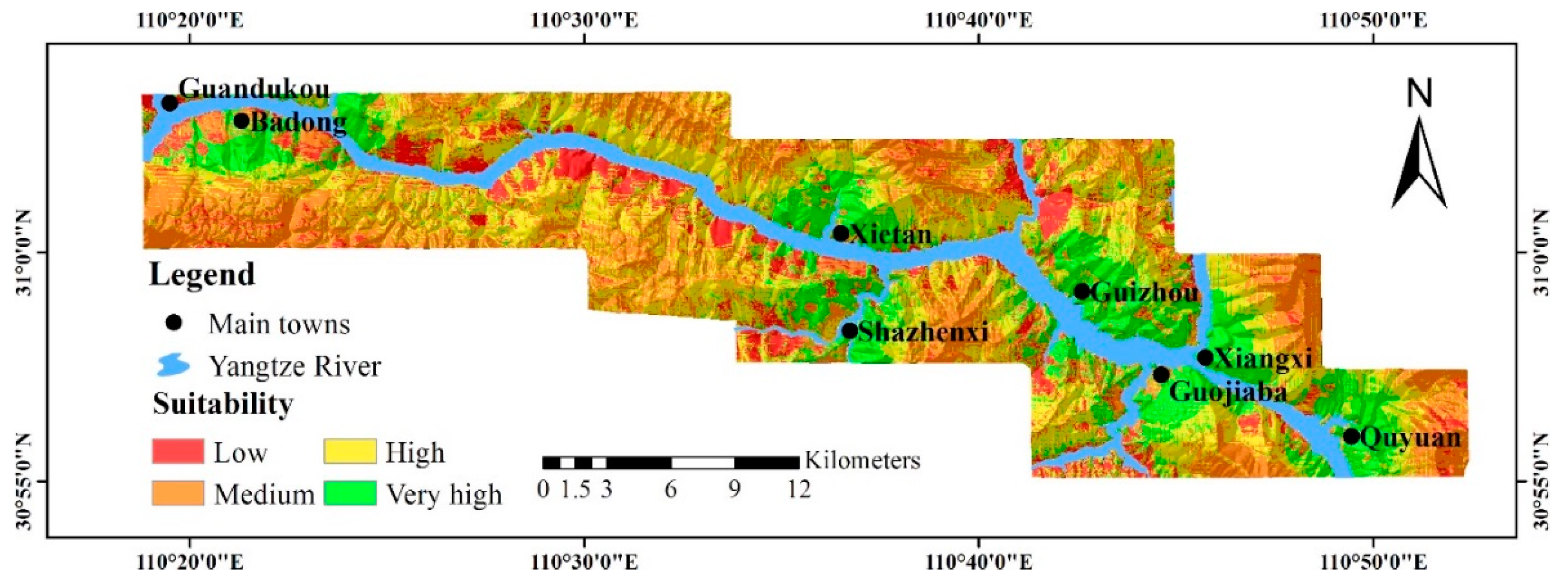
4.2. The Suitability for Urban Development
- near the county of Badong, southwest south and southeast of this county.
- near the county of Xietan, west, northwest, north, northeast and east of this county.
- near the county of Shazhenxi, northwest, north, northeast and south of this county.
- near the county of Guizhou, north, northeast, east and southeast of this county.
- near the county of Guojiaba, south and southeast of this county.
- near the county of Xiangxi, north, northeast and east of this county.
- near the county of Quyuan, northwest, north, northeast, east and southeast of this county.
5. Conclusions
Acknowledgments
Author Contributions
Conflicts of Interest
References
- Liu, C.; Liu, Y.; Wen, M.; Li, T.; Lian, J.; Qin, S. Geo-hazard initiation and assessment in the three gorges reservoir. In Landslide Disaster Mitigation in Three Gorges Reservoir, China; Springer: Berlin/Heidelberg, Germany, 2009; pp. 3–40. [Google Scholar]
- Tangestani, M.H. A comparative study of Dempster-Shafer and fuzzy models for landslide susceptibility mapping using a GIS: An experience from Zagros Mountains, SW Iran. J. Asian Earth Sci. 2009, 35, 66–73. [Google Scholar] [CrossRef]
- Mantovani, F.; Soeters, R.; Van Westen, C.J. Remote sensing techniques for landslide studies and hazard zonation in Europe. Geomorphology 1996, 15, 213–225. [Google Scholar] [CrossRef]
- Metternicht, G.; Hurni, L.; Gogu, R. Remote sensing of landslides: An analysis of the potential contribution to geo-spatial systems for hazard assessment in mountainous environments. Remote Sens. Environ. 2005, 98, 284–303. [Google Scholar] [CrossRef]
- Scaioni, M.; Longoni, L.; Melillo, V.; Papini, M. Remote sensing for landslide investigations: An overview of recent achievements and perspectives. Remote Sens. 2014, 6, 9600. [Google Scholar] [CrossRef]
- Bui, D.T.; Tuan, T.A.; Klempe, H.; Pradhan, B.; Revhaug, I. Spatial prediction models for shallow landslide hazards: A comparative assessment of the efficacy of support vector machines, artificial neural networks, kernel logistic regression, and logistic model tree. Landslides 2016, 13, 361–378. [Google Scholar]
- Regmi, N.R.; Giardino, J.R.; Vitek, J.D. Assessing susceptibility to landslides: Using models to understand observed changes in slopes. Geomorphology 2010, 122, 25–38. [Google Scholar] [CrossRef]
- Kamp, U.; Growley, B.J.; Khattak, G.A.; Owen, L.A. GIS-based landslide susceptibility mapping for the 2005 kashmir earthquake region. Geomorphology 2008, 101, 631–642. [Google Scholar] [CrossRef]
- Yalcin, A. GIS-based landslide susceptibility mapping using analytical hierarchy process and bivariate statistics in Ardesen (Turkey): Comparisons of results and confirmations. CATENA 2008, 72, 1–12. [Google Scholar] [CrossRef]
- Zhang, G.; Cai, Y.; Zheng, Z.; Zhen, J.; Liu, Y.; Huang, K. Integration of the statistical index method and the analytic hierarchy process technique for the assessment of landslide susceptibility in Huizhou, China. CATENA 2016, 142, 233–244. [Google Scholar] [CrossRef]
- Gokceoglu, M.E.C. Assessment of landslide susceptibility for a landslide-prone area (north of Yenice, NW Turkey) by fuzzy approach. Environ. Geol. 2002, 41, 720–730. [Google Scholar] [CrossRef]
- Jiang, H.; Eastman, J.R. Application of fuzzy measures in multi-criteria evaluation in GIS. Int. J. Geogr. Inf. Sci. 2000, 14, 173–184. [Google Scholar] [CrossRef]
- Pradhan, A.M.S.; Kim, Y.T. Evaluation of a combined spatial multi-criteria evaluation model and deterministic model for landslide susceptibility mapping. CATENA 2016, 140, 125–139. [Google Scholar] [CrossRef]
- Akgun, A.; Dag, S.; Bulut, F. Landslide susceptibility mapping for a landslide-prone area (Findikli, NE of Turkey) by likelihood-frequency ratio and weighted linear combination models. Environ. Geol. 2008, 54, 1127–1143. [Google Scholar] [CrossRef]
- Ayalew, L.; Yamagishi, H.; Marui, H.; Kanno, T. Landslides in Sado Island of Japan: Part II. GIS-based susceptibility mapping with comparisons of results from two methods and verifications. Eng. Geol. 2005, 81, 432–445. [Google Scholar] [CrossRef]
- Feizizadeh, B.; Blaschke, T.; Nazmfar, H. GIS-based ordered weighted averaging and Dempster-Shafer methods for landslide susceptibility mapping in the Urmia Lake Basin, Iran. Int. J. Digit. Earth 2012, 7, 688–708. [Google Scholar] [CrossRef]
- Ferretti, V.; Pomarico, S. Ecological land suitability analysis through spatial indicators: An application of the analytic network process technique and ordered weighted average approach. Ecol. Indic. 2013, 34, 507–519. [Google Scholar] [CrossRef]
- Ayalew, L.; Yamagishi, H. The application of GIS-based logistic regression for landslide susceptibility mapping in the Kakuda-Yahiko Mountains, central Japan. Geomorphology 2005, 65, 15–31. [Google Scholar] [CrossRef]
- Chung, C.-J.F.; Fabbri, A.G. The representation of geoscience information for data integration. Nat. Resour. Res. 1993, 2, 122–139. [Google Scholar] [CrossRef]
- Chung, C.; Fabbri, A. Three bayesian prediction models for landslide hazard. In Proceedings of the International Association for Mathematical Geology 1998 Annual Meeting, Ischia, Italy, 3–7 October 1998. [Google Scholar]
- Chung, C.-J.F.; Fabbri, A.G. Probabilistic prediction models for landslide hazard mapping. Photogramm. Eng. Remote Sens. 1999, 65, 1389–1399. [Google Scholar]
- Saha, A.K.; Gupta, R.P.; Sarkar, I.; Arora, M.K.; Csaplovics, E. An approach for GIS-based statistical landslide susceptibility zonation—With a case study in the Himalayas. Landslides 2005, 2, 61–69. [Google Scholar] [CrossRef]
- Guillard, C.; Zezere, J. Landslide susceptibility assessment and validation in the framework of municipal planning in Portugal: The case of Loures municipality. Environ. Manag. 2012, 50, 721–735. [Google Scholar] [CrossRef] [PubMed]
- Pradhan, B.; Lee, S. Landslide susceptibility assessment and factor effect analysis: Backpropagation artificial neural networks and their comparison with frequency ratio and bivariate logistic regression modelling. Environ. Model. Softw. 2010, 25, 747–759. [Google Scholar] [CrossRef]
- Pradhan, B.; Oh, H.-J.; Buchroithner, M. Weights-of-evidence model applied to landslide susceptibility mapping in a tropical hilly area. Geomat. Nat. Hazards Risk 2010, 1, 199–223. [Google Scholar] [CrossRef]
- Lee, S.; Choi, J. Landslide susceptibility mapping using GIS and the weight-of-evidence model. Int. J. Geogr. Inf. Sci. 2004, 18, 789–814. [Google Scholar] [CrossRef]
- Regmi, N.R.; Giardino, J.R.; Vitek, J.D. Modeling susceptibility to landslides using the weight of evidence approach: Western Colorado, USA. Geomorphology 2010, 115, 172–187. [Google Scholar] [CrossRef]
- Blahut, J.; van Westen, C.J.; Sterlacchini, S. Analysis of landslide inventories for accurate prediction of debris-flow source areas. Geomorphology 2010, 119, 36–51. [Google Scholar] [CrossRef]
- Hong, H.; Ilia, I.; Tsangaratos, P.; Chen, W.; Xu, C. A hybrid fuzzy weight of evidence method in landslide susceptibility analysis on the Wuyuan area, China. Geomorphology 2017, 290, 1–16. [Google Scholar] [CrossRef]
- Pradhan, B.; Lee, S. Delineation of landslide hazard areas on Penang Island, Malaysia, by using frequency ratio, logistic regression, and artificial neural network models. Environ. Earth Sci. 2009, 60, 1037–1054. [Google Scholar] [CrossRef]
- Lee, S.; Pradhan, B. Landslide hazard mapping at Selangor, Malaysia using frequency ratio and logistic regression models. Landslides 2006, 4, 33–41. [Google Scholar] [CrossRef]
- Pradhan, B.; Chaudhari, A.; Adinarayana, J.; Buchroithner, M.F. Soil erosion assessment and its correlation with landslide events using remote sensing data and GIS: A case study at Penang Island, Malaysia. Environ. Monit. Assess. 2012, 184, 715–727. [Google Scholar] [CrossRef] [PubMed]
- Pourghasemi, H.; Pradhan, B.; Gokceoglu, C.; Moezzi, K.D. A comparative assessment of prediction capabilities of Dempster-Shafer and weights-of-evidence models in landslide susceptibility mapping using GIS. Geomat. Nat. Hazards Risk 2013, 4, 93–118. [Google Scholar] [CrossRef] [Green Version]
- Corominas, J.; van Westen, C.; Frattini, P.; Cascini, L.; Malet, J.P.; Fotopoulou, S.; Catani, F.; Van Den Eeckhaut, M.; Mavrouli, O.; Agliardi, F.; et al. Recommendations for the quantitative analysis of landslide risk. Bull. Eng. Geol. Environ. 2014, 73, 209–263. [Google Scholar] [CrossRef] [Green Version]
- Zêzere, J.L.; Pereira, S.; Melo, R.; Oliveira, S.C.; Garcia, R.A.C. Mapping landslide susceptibility using data-driven methods. Sci. Total Environ. 2017, 589, 250–267. [Google Scholar] [CrossRef] [PubMed]
- Chen, Z.; Wang, J. Landslide hazard mapping using logistic regression model in Mackenzie Valley, Canada. Nat. Hazards 2007, 42, 75–89. [Google Scholar] [CrossRef]
- Can, T.; Nefeslioglu, H.A.; Gokceoglu, C.; Sonmez, H.; Duman, T.Y. Susceptibility assessments of shallow earthflows triggered by heavy rainfall at three catchments by logistic regression analyses. Geomorphology 2005, 72, 250–271. [Google Scholar] [CrossRef]
- Tsangaratos, P.; Ilia, I. Comparison of a logistic regression and naïve bayes classifier in landslide susceptibility assessments: The influence of models complexity and training dataset size. CATENA 2016, 145, 164–179. [Google Scholar] [CrossRef]
- Gorum, T.; Gonencgil, B.; Gokceoglu, C.; Nefeslioglu, H.A. Implementation of reconstructed geomorphologic units in landslide susceptibility mapping: The Melen Gorge (NW Turkey). Nat. Hazards 2008, 46, 323–351. [Google Scholar] [CrossRef]
- Tunusluoglu, M.C.; Gokceoglu, C.; Nefeslioglu, H.A.; Sonmez, H. Extraction of potential debris source areas by logistic regression technique: A case study from Barla, Besparmak and Kapi mountains (NW Taurids, Turkey). Environ. Geol. 2007, 54, 9–22. [Google Scholar] [CrossRef]
- Nefeslioglu, H.A.; Gokceoglu, C.; Sonmez, H. An assessment on the use of logistic regression and artificial neural networks with different sampling strategies for the preparation of landslide susceptibility maps. Eng. Geol. 2008, 97, 171–191. [Google Scholar] [CrossRef]
- Choi, J.; Oh, H.-J.; Lee, H.-J.; Lee, C.; Lee, S. Combining landslide susceptibility maps obtained from frequency ratio, logistic regression, and artificial neural network models using aster images and GIS. Eng. Geol. 2012, 124, 12–23. [Google Scholar] [CrossRef]
- Akgun, A.; Kincal, C.; Pradhan, B. Application of remote sensing data and GIS for landslide risk assessment as an environmental threat to Izmir city (west Turkey). Environ. Monit. Assess. 2012, 184, 5453–5470. [Google Scholar] [CrossRef] [PubMed]
- Dong, J.-J.; Tung, Y.-H.; Chen, C.-C.; Liao, J.-J.; Pan, Y.-W. Discriminant analysis of the geomorphic characteristics and stability of landslide dams. Geomorphology 2009, 110, 162–171. [Google Scholar] [CrossRef]
- Mihai, B.; Sandric, I.; Savulescu, I.; Chitu, Z. Detailed mapping of landslide susceptibility for urban planning purposes in carpathian and subcarpathian towns of Romania. In Cartography in Central and Eastern Europe: CEE 2009; Gartner, G., Ortag, F., Eds.; Springer: Berlin/Heidelberg, Germany, 2010; pp. 417–429. [Google Scholar]
- Yesilnacar, E.; Süzen, M.L. A land-cover classification for landslide susceptibility mapping by using feature components. Int. J. Remote Sens. 2006, 27, 253–275. [Google Scholar] [CrossRef]
- Saito, H.; Nakayama, D.; Matsuyama, H. Comparison of landslide susceptibility based on a decision-tree model and actual landslide occurrence: The Akaishi mountains, Japan. Geomorphology 2009, 109, 108–121. [Google Scholar] [CrossRef]
- Pradhan, B. A comparative study on the predictive ability of the decision tree, support vector machine and neuro-fuzzy models in landslide susceptibility mapping using GIS. Comput. Geosci. 2013, 51, 350–365. [Google Scholar] [CrossRef] [Green Version]
- Catani, F.; Lagomarsino, D.; Segoni, S.; Tofani, V. Landslide susceptibility estimation by random forests technique: Sensitivity and scaling issues. Nat. Hazards Earth Syst. 2013, 13, 2815–2831. [Google Scholar] [CrossRef]
- Vorpahl, P.; Elsenbeer, H.; Märker, M.; Schröder, B. How can statistical models help to determine driving factors of landslides? Ecol. Model. 2012, 239, 27–39. [Google Scholar] [CrossRef]
- Pourghasemi, H.R.; Kerle, N. Random forests and evidential belief function-based landslide susceptibility assessment in Western Mazandaran Province, Iran. Environ. Earth Sci. 2016, 75, 185. [Google Scholar] [CrossRef]
- Chen, C.-H.; Ke, C.-C.; Wang, C.-L. A back-propagation network for the assessment of susceptibility to rock slope failure in the eastern portion of the southern cross-island highway in Taiwan. Environ. Geol. 2009, 57, 723–733. [Google Scholar] [CrossRef]
- Pradhan, B.; Lee, S. Landslide risk analysis using artificial neural network model focussing on different training sites. Int. J. Phys. Sci. 2009, 4, 1–15. [Google Scholar]
- Pradhan, B.; Youssef, A.; Varathrajoo, R. Approaches for delineating landslide hazard areas using different training sites in an advanced artificial neural network model. Geospat. Inf. Sci. 2010, 13, 93–102. [Google Scholar] [CrossRef]
- Arnone, E.; Francipane, A.; Scarbaci, A.; Puglisi, C.; Noto, L.V. Effect of raster resolution and polygon-conversion algorithm on landslide susceptibility mapping. Environ. Model. Softw. 2016, 84, 467–481. [Google Scholar] [CrossRef]
- Pham, B.T.; Tien Bui, D.; Prakash, I.; Dholakia, M.B. Hybrid integration of multilayer perceptron neural networks and machine learning ensembles for landslide susceptibility assessment at Himalayan area (India) using GIS. CATENA 2017, 149, 52–63. [Google Scholar] [CrossRef]
- Tien Bui, D.; Pradhan, B.; Lofman, O.; Revhaug, I. Landslide susceptibility assessment in Vietnam using support vector machines, decision tree, and naïve bayes models. Math. Probl. Eng. 2012, 2012, 1–26. [Google Scholar] [CrossRef]
- Yilmaz, I. Comparison of landslide susceptibility mapping methodologies for Koyulhisar, Turkey: Conditional probability, logistic regression, artificial neural networks, and support vector machine. Environ. Earth Sci. 2010, 61, 821–836. [Google Scholar] [CrossRef]
- Tien Bui, D.; Pradhan, B.; Lofman, O.; Revhaug, I.; Dick, O.B. Landslide susceptibility assessment in the Hoa Binh Province of Vietnam: A comparison of the levenberg-marquardt and bayesian regularized neural networks. Geomorphology 2012, 171–172, 12–29. [Google Scholar] [CrossRef]
- Hughes, G. On the mean accuracy of statistical pattern recognizers. IEEE Trans. Inf. Theory 1968, 14, 55–63. [Google Scholar] [CrossRef]
- Kavzoglu, T.; Kutlug Sahin, E.; Colkesen, I. Selecting optimal conditioning factors in shallow translational landslide susceptibility mapping using genetic algorithm. Eng. Geol. 2015, 192, 101–112. [Google Scholar] [CrossRef]
- Guzzetti, F.; Carrara, A.; Cardinali, M.; Reichenbach, P. Landslide hazard evaluation: A review of current techniques and their application in a multi-scale study, central Italy. Geomorphology 1999, 31, 181–216. [Google Scholar] [CrossRef]
- Pradhan, B.; Lee, S.; Buchroithner, M.F. A GIS-based back-propagation neural network model and its cross-application and validation for landslide susceptibility analyses. Comput. Environ. Urban Syst. 2010, 34, 216–235. [Google Scholar] [CrossRef]
- Oh, H.-J.; Pradhan, B. Application of a neuro-fuzzy model to landslide-susceptibility mapping for shallow landslides in a tropical hilly area. Comput. Geosci. 2011, 37, 1264–1276. [Google Scholar] [CrossRef]
- Das, I.; Stein, A.; Kerle, N.; Dadhwal, V. Probabilistic landslide hazard assessment using homogeneous susceptible units (HSU) along a national highway corridor in the northern Himalayas, India. Landslides 2011, 8, 293–308. [Google Scholar] [CrossRef]
- Erener, A.; Düzgün, H.S.B. Improvement of statistical landslide susceptibility mapping by using spatial and global regression methods in the case of More and Romsdal (Norway). Landslides 2010, 7, 55–68. [Google Scholar] [CrossRef]
- Yu, X.; Wang, Y.; Niu, R.; Hu, Y. A combination of geographically weighted regression, particle swarm optimization and support vector machine for landslide susceptibility mapping: A case study at Wanzhou in the Three Gorges Area, China. Int. J. Environ. Res. Public Health 2016, 13, 487. [Google Scholar] [CrossRef] [PubMed]
- Shannon, C.E. A mathematical theory of communication. ACM SIGMOBILE Mobile Comput. Commun. Rev. 2001, 5, 3–55. [Google Scholar] [CrossRef]
- Constantin, M.; Bednarik, M.; Jurchescu, M.C.; Vlaicu, M. Landslide susceptibility assessment using the bivariate statistical analysis and the index of entropy in the Sibiciu Basin (Romania). Environ. Earth Sci. 2010, 63, 397–406. [Google Scholar] [CrossRef]
- Bednarik, M.; Magulová, B.; Matys, M.; Marschalko, M. Landslide susceptibility assessment of the Kra’ovany-Liptovský Mikuláš railway case study. Phys. Chem. Earth Parts A/B/C 2010, 35, 162–171. [Google Scholar] [CrossRef]
- Kanungo, D.P.; Sarkar, S.; Sharma, S. Combining neural network with fuzzy, certainty factor and likelihood ratio concepts for spatial prediction of landslides. Nat. Hazards 2011, 59, 1491–1512. [Google Scholar] [CrossRef]
- Likas, A.; Vlassis, N.; Verbeek, J.J. The global K-means clustering algorithm. Pattern Recogn. 2003, 36, 451–461. [Google Scholar] [CrossRef]
- Ding, C.; He, X. K-means clustering via principal component analysis. In Proceedings of the Twenty-First International Conference on Machine Learning, Banff, AB, Canada, 4–8 July 2004. [Google Scholar]
- Alsabti, K.; Ranka, S.; Singh, V. An efficient K-means clustering algorithm. Electr. Eng. Comput. Sci. 1997, 43. [Google Scholar]
- O’brien, R.M. A caution regarding rules of thumb for variance inflation factors. Qual. Quant. 2007, 41, 673–690. [Google Scholar] [CrossRef]
- Marquaridt, D.W. Generalized inverses, ridge regression, biased linear estimation, and nonlinear estimation. Technometrics 1970, 12, 591–612. [Google Scholar] [CrossRef]
- Das, I.; Sahoo, S.; van Westen, C.; Stein, A.; Hack, R. Landslide susceptibility assessment using logistic regression and its comparison with a rock mass classification system, along a road section in the northern Himalayas (India). Geomorphology 2010, 114, 627–637. [Google Scholar] [CrossRef]
- Bai, S.-B.; Wang, J.; Lü, G.-N.; Zhou, P.-G.; Hou, S.-S.; Xu, S.-N. GIS-based logistic regression for landslide susceptibility mapping of the Zhongxian segment in the Three Gorges Area, China. Geomorphology 2010, 115, 23–31. [Google Scholar] [CrossRef]
- Nandi, A.; Shakoor, A. A GIS-based landslide susceptibility evaluation using bivariate and multivariate statistical analyses. Eng. Geol. 2010, 110, 11–20. [Google Scholar] [CrossRef]
- Dai, F.; Lee, C.; Ngai, Y.Y. Landslide risk assessment and management: An overview. Eng. Geol. 2002, 64, 65–87. [Google Scholar] [CrossRef]
- Gorsevski, P.V.; Gessler, P.E.; Boll, J.; Elliot, W.J.; Foltz, R.B. Spatially and temporally distributed modeling of landslide susceptibility. Geomorphology 2006, 80, 178–198. [Google Scholar] [CrossRef]
- Akgun, A.; Sezer, E.A.; Nefeslioglu, H.A.; Gokceoglu, C.; Pradhan, B. An easy-to-use MATLAB program (MamLand) for the assessment of landslide susceptibility using a Mamdani fuzzy algorithm. Comput. Geosci. 2012, 38, 23–34. [Google Scholar] [CrossRef]
- Kundu, S.; Saha, A.; Sharma, D.; Pant, C. Remote sensing and GIS based landslide susceptibility assessment using binary logistic regression model: A case study in the Ganeshganga watershed, Himalayas. J. Indian Soc. Remote Sens. 2013, 41, 697–709. [Google Scholar] [CrossRef]
- Sdao, F.; Lioi, D.; Pascale, S.; Caniani, D.; Mancini, I. Landslide susceptibility assessment by using a neuro-fuzzy model: A case study in the Rupestrian heritage rich area of Matera. Nat. Hazards Earth Syst. 2013, 13, 395. [Google Scholar] [CrossRef]
- Fawcett, T. An introduction to ROC analysis. Pattern Recogn. Lett. 2006, 27, 861–874. [Google Scholar] [CrossRef]
- Tsangaratos, P.; Ilia, I.; Hong, H.; Chen, W.; Xu, C. Applying information theory and GIS-based quantitative methods to produce landslide susceptibility maps in Nancheng county, China. Landslides 2016, 1–21. [Google Scholar] [CrossRef]
- Bathrellos, G.D.; Gaki-Papanastassiou, K.; Skilodimou, H.D.; Papanastassiou, D.; Chousianitis, K.G. Potential suitability for urban planning and industry development using natural hazard maps and geological-geomorphological parameters. Environ. Earth Sci. 2012, 66, 537–548. [Google Scholar] [CrossRef]
- Bathrellos, G.D.; Skilodimou, H.D.; Chousianitis, K.; Youssef, A.M.; Pradhan, B. Suitability estimation for urban development using multi-hazard assessment map. Sci. Total Environ. 2017, 575, 119–134. [Google Scholar] [CrossRef] [PubMed]
- Dai, F.; Lee, C.; Zhang, X. GIS-based geo-environmental evaluation for urban land-use planning: A case study. Eng. Geol. 2001, 61, 257–271. [Google Scholar] [CrossRef]
- Svoray, T.; Bar, P.; Bannet, T. Urban land-use allocation in a mediterranean ecotone: Habitat heterogeneity model incorporated in a GIS using a multi-criteria mechanism. Landsc. Urban Plan. 2005, 72, 337–351. [Google Scholar] [CrossRef]
- Wang, X.; Zhong, X.; Liu, S.; Liu, J.; Wang, Z.; Li, M. Regional assessment of environmental vulnerability in the Tibetan Plateau: Development and application of a new method. J. Arid Environ. 2008, 72, 1929–1939. [Google Scholar] [CrossRef]


| Causative Factor | Information Coefficient | ||||
|---|---|---|---|---|---|
| 2 Classes | 3 Classes | 4 Classes | 5 Classes | 6 Classes | |
| Elevation | 0.8655 | 0.3912 | 0.4209 | NC | NC |
| Distance to river | 0.8040 | 0.4542 | 0.3068 | 0.2743 | NC |
| NDVI | 0.2898 | 0.1578 | 0.1223 | 0.1172 | 0.1053 |
| NDWI | 0.2776 | 0.1439 | 0.1486 | 0.1428 | 0.1175 |
| TRI | 0.2343 | 0.2270 | 0.2472 | 0.2398 | NC |
| TPI | 0.0011 | 0.0715 | 0.0889 | 0.1021 | 0.1089 |
| Slope gradient | 0.1144 | 0.1229 | 0.1140 | 0.1123 | 0.1180 |
| Distance to fault | 0.0193 | 0.0037 | 0.0048 | 0.0322 | 0.0181 |
| Catchment area | 0.0531 | 0.0386 | 0.0294 | 0.0315 | 0.0360 |
| Catchment slope | 0.1175 | 0.1350 | 0.1230 | 0.1279 | 0.1258 |
| Terrain curvature | 0.0080 | 0.0384 | 0.0640 | 0.0808 | 0.0933 |
| TWI | 0.0858 | 0.1798 | 0.1690 | 0.1424 | 0.1539 |
| Terrain surface convexity | 0.0582 | 0.0847 | 0.0933 | 0.0781 | 0.0729 |
| Terrain surface texture | 0.3848 | 0.3495 | 0.3139 | 0.3040 | 0.2940 |
| Category | Value Range | Description | Stability |
|---|---|---|---|
| 1 | Basically no landslides occurred | stable | |
| 2 | Landslides are less likely to occur | relatively stable | |
| 3 | Uncertain whether landslides will occur | uncertain | |
| 4 | Landslides are more likely to occur | unstable | |
| 5 | The possibility of landslides is great | extremely unstable |
| Causative Factor | Classes | Percentage of Landslide | Percentage of Class | CF |
|---|---|---|---|---|
| Elevation | 80~700 | 99.00 | 65.50 | 0.3599 |
| >700~2000 | 1.00 | 34.50 | −0.9728 | |
| Distance to river | <2000 | 96.80 | 48.57 | 0.5300 |
| 2000~6900 | 3.20 | 51.43 | −0.9412 | |
| NDVI | −0.7186~0.4140 | 16.24 | 4.46 | 0.7713 |
| >0.4140~0.9190 | 83.76 | 95.54 | −0.1301 | |
| NDWI | −0.8879~0.4503 | 88.29 | 96.79 | 0.0929 |
| >0.4503~0.8025 | 11.71 | 3.21 | 0.7718 | |
| Catchment area | 900~18,590 | 96.13 | 91.52 | −0.0624 |
| >18,590~412,609 | 3.87 | 8.48 | 0.4134 | |
| Terrain surface texture | 4.4474~28.4901 | 82.07 | 45.10 | 0.4792 |
| >28.4901~61.9701 | 17.93 | 54.90 | −0.6869 | |
| Slope gradient | <20 | 48.77 | 35.17 | 0.2967 |
| 20~35 | 44.61 | 44.25 | 0.0086 | |
| >35~75 | 6.62 | 20.58 | −0.6920 | |
| Lithology | mudstone, shale and Quaternary deposits | 3.94 | 22.48 | −0.8660 |
| sandstones and thinly bedded limestones | 51.82 | 26.97 | 0.5153 | |
| limestones and massive sandstones | 44.24 | 50.55 | −0.1257 | |
| TWI | 0.8704~3.4408 | 23.12 | 51.64 | −0.5676 |
| >3.4408~6.2721 | 76.49 | 47.49 | 0.4033 | |
| >6.2721~10.4071 | 0.39 | 0.87 | −0.5626 | |
| Catchment slope | <0.3224 | 36.43 | 28.02 | 0.2457 |
| 0.3224~0.4946 | 56.68 | 47.52 | 0.1719 | |
| >0.4946~1.1306 | 6.89 | 24.46 | −0.7308 | |
| TRI | <8.8293 | 58.80 | 39.26 | 0.3535 |
| 8.8293~15.0834 | 35.76 | 41.89 | −0.1542 | |
| >15.0834~26.1201 | 5.26 | 16.50 | −0.6947 | |
| >26.1201~94.1794 | 0.18 | 2.35 | −0.9277 | |
| Terrain surface convexity | >13.9169~42.4579 | 12.13 | 5.10 | 0.6168 |
| >42.4579~48.8004 | 31.42 | 25.02 | 0.2167 | |
| >48.8004~53.7838 | 41.06 | 43.07 | −0.0495 | |
| >53.7838~71.9051 | 15.39 | 26.81 | −0.4412 | |
| Distance to fault | <1200 | 24.54 | 28.50 | −0.1464 |
| 1200~2400 | 22.32 | 27.37 | −0.1940 | |
| >2400~3600 | 29.61 | 22.88 | 0.2418 | |
| >3600~5400 | 20.84 | 16.01 | 0.2463 | |
| >5400~8700 | 2.69 | 5.24 | −0.5011 | |
| TPI | −90.8220~−18.5199 | 0.52 | 2.13 | −0.7665 |
| >−18.5199~−8.4604 | 6.04 | 10.30 | −0.4283 | |
| >−8.4604~−2.7133 | 26.97 | 22.60 | 0.1724 | |
| >−2.7133~4.1138 | 48.00 | 35.04 | 0.2873 | |
| >4.1138~12.2871 | 17.17 | 23.56 | −0.2835 | |
| >12.2871~70.1288 | 1.30 | 6.37 | −0.8060 | |
| Terrain curvature | −2.1060~−0.4418 | 0.21 | 1.07 | −0.8173 |
| >−0.4418~−0.1991 | 3.83 | 7.44 | −0.5006 | |
| >−0.1991~−0.0604 | 20.45 | 20.08 | 0.0194 | |
| >−0.0604~0.0782 | 56.76 | 45.41 | 0.2128 | |
| >0.0782~0.2863 | 17.65 | 22.28 | −0.2178 | |
| >0.2863~2.3318 | 1.10 | 3.72 | −0.7184 | |
| Slope aspect | Flat | 0.26 | 0.57 | −0.5560 |
| North | 23.54 | 14.83 | 0.3936 | |
| North–East | 15.95 | 12.57 | 0.2249 | |
| East | 9.67 | 11.86 | −0.1940 | |
| South–East | 7.27 | 10.62 | −0.3292 | |
| South | 13.52 | 12.47 | 0.0826 | |
| South-West | 6.43 | 10.86 | −0.4234 | |
| West | 9.46 | 14.52 | −0.3620 | |
| North–West | 13.90 | 11.70 | 0.1690 | |
| Slope form | V/V | 29.74 | 28.71 | 0.0367 |
| GE/V | 2.70 | 1.63 | 0.4238 | |
| X/V | 10.60 | 11.15 | −0.0522 | |
| V/GR | 4.05 | 3.54 | 0.1340 | |
| GE/GR | 1.30 | 0.58 | 0.5896 | |
| X/GR | 3.27 | 3.05 | 0.0728 | |
| V/X | 13.05 | 13.84 | −0.0605 | |
| GE/X | 3.72 | 2.37 | 0.3867 | |
| X/X | 31.57 | 35.13 | −0.1100 |
| Causative Factor/Intercept | No Clustering | |||||||
|---|---|---|---|---|---|---|---|---|
| Cluster 1 | Cluster 2 | Cluster 3 | ||||||
| Intercept | −8.125 | −8.783 | −17.097 | 1.415 | ||||
| SE | RC | SE | RC | SE | RC | SE | RC | |
| Elevation | √ | 1.838 | ||||||
| Distance to river | √ | 2.801 | √ | 4.473 | ||||
| NDVI | √ | −0.597 | √ | 0.709 | ||||
| NDWI | √ | 0.276 | ||||||
| Catchment area | √ | −0.156 | ||||||
| Terrain surface texture | √ | 1.295 | √ | 0.906 | √ | 0.908 | ||
| Slope gradient | √ | 0.255 | √ | 5.476 | √ | 4.256 | ||
| Lithology | √ | −1.191 | ||||||
| TWI | √ | 0.671 | √ | 4.470 | √ | −13.190 | ||
| Catchment slope | √ | 0.400 | √ | 3.643 | ||||
| TRI | √ | 1.340 | √ | 3.859 | ||||
| Terrain surface convexity | √ | 0.836 | √ | 13.433 | ||||
| Distance to fault | √ | 0.286 | ||||||
| TPT | √ | 0.573 | √ | 1.819 | ||||
| Terrain curvature | √ | −0.648 | √ | −1.322 | √ | −0.346 | ||
| Slope aspect | √ | −0.297 | √ | −0.898 | ||||
| Slope form | √ | 0.012 | √ | −0.184 | ||||
| Causative Factor | Cluster 1 | Cluster 2 | Cluster 3 |
|---|---|---|---|
| TOL/VIF | |||
| Elevation | |||
| Distance to river | 0.940/1.064 | ||
| NDVI | 0.944/1.059 | ||
| NDWI | |||
| Catchment area | |||
| Terrain surface texture | 0.977/1.023 | 0.944/1.060 | |
| Slope gradient | 0.648/1.543 | 0.402/2.489 | |
| Lithology | |||
| TWI | 0.741/1.350 | 0.408/2.451 | |
| Catchment slope | 0.612/1.634 | ||
| TRI | 0.401/2.494 | ||
| Terrain surface convexity | 0.538/1.860 | ||
| Distance to fault | |||
| TPI | 0.775/1.291 | ||
| Terrain curvature | 0.812/1.231 | 0.907/1.102 | |
| Slope aspect | 0.961/1.041 | ||
| Slope form | 0.999/1.001 | ||
| Methods | Overall Accuracy |
|---|---|
| LR | 80.26% |
| SVM | 83.74% |
| DT | 84.13% |
| LR_K3 | 85.32% |
| Causative Factor/Intercept | ||||||||||||
|---|---|---|---|---|---|---|---|---|---|---|---|---|
| Cluster 1 | Cluster 2 | Cluster 1 | Cluster 2 | Cluster 3 | Cluster 4 | |||||||
| Intercept | −3.600 | −0.508 | −17.628 | −30.784 | −50.719 | −12.063 | ||||||
| SE | RC | SE | RC | SE | RC | SE | RC | SE | RC | SE | RC | |
| Elevation | √ | 3.321 | √ | 4.392 | √ | 20.754 | ||||||
| Distance to river | √ | 4.473 | √ | 7.241 | √ | 13.396 | √ | 3.392 | ||||
| NDVI | √ | 0.709 | ||||||||||
| NDWI | √ | 3.447 | ||||||||||
| Catchment area | ||||||||||||
| Terrain surface texture | √ | 0.906 | √ | 0.908 | √ | 17.378 | √ | 2.841 | ||||
| Slope gradient | √ | 5.476 | ||||||||||
| Lithology | √ | 1.350 | √ | 3.513 | ||||||||
| TWI | √ | 4.470 | √ | 14.754 | √ | −3.863 | √ | 0.400 | ||||
| Catchment slope | √ | 3.643 | √ | 3.990 | ||||||||
| TRI | ||||||||||||
| Terrain surface convexity | √ | 7.693 | √ | 31.940 | ||||||||
| Distance to fault | ||||||||||||
| TPT | √ | 1.819 | √ | 3.560 | √ | −2.669 | √ | 0.778 | ||||
| Terrain curvature | √ | −1.322 | √ | −1.286 | ||||||||
| Slope aspect | √ | −0.898 | √ | −1.151 | ||||||||
| Slope form | √ | −0.184 | √ | −0.519 | ||||||||
| Causative Factor | (TOL/VIF) | (TOL/VIF) | ||||
|---|---|---|---|---|---|---|
| Cluster 1 | Cluster 2 | Cluster 1 | Cluster 2 | Cluster 3 | Cluster 4 | |
| Elevation | 0.569/1.756 | 0.861/1.162 | 0.464/2.154 | |||
| Distance to river | 0.934/1.070 | 0.563/1.777 | 0.406/2.462 | 0.985/1.016 | ||
| NDVI | ||||||
| NDWI | 0.915/1.093 | 0.969/1.032 | ||||
| Catchment area | ||||||
| Terrain surface texture | 0.975/1.026 | 0.670/1.493 | 0.946/1.057 | |||
| Slope gradient | ||||||
| Lithology | 0.977/1.023 | 0.852/1.173 | 0.864/1.157 | |||
| TWI | 0.789/1.268 | 0.949/1.054 | 0.774/1.291 | 0.627/1.594 | ||
| Catchment slope | 0.806/1.240 | 0.632/1.581 | ||||
| TRI | ||||||
| Terrain surface convexity | 0.958/1.043 | 0.780/1.282 | ||||
| Distance to fault | ||||||
| TPI | 0.975/1.026 | 0.931/1.074 | 0.912/1.097 | 0.638/1.567 | ||
| Terrain curvature | 0.908/1.101 | 0.998/1.002 | ||||
| Slope aspect | 0.997/1.003 | 0.879/1.138 | ||||
| Slope form | 0.685/1.460 | |||||
| Clusters | Statistics | ||||
|---|---|---|---|---|---|
| −2ln Likelihood | −2ln L0 | Goodness of Fit | Pseudo R2 | ||
| No clustering | 68,666.849 | 36,819.425 | 69,332.399 | 0.463 | |
| Cluster 1 | 15,559.511 | 8542.172 | 215.389 | 0.451 | |
| Cluster 2 | 27,105.308 | 10,245.806 | 2833.666 | 0.622 | |
| Cluster 1 | 21,731.018 | 1738.480 | 1887.318 | 0.920 | |
| Cluster 2 | 62,526.249 | 46,769.634 | 3962.812 | 0.252 | |
| Cluster 3 | 12,830.029 | 3412.788 | 2805.024 | 0.734 | |
| Cluster 1 | 24,014.293 | 17,722.546 | 1954.458 | 0.262 | |
| Cluster 2 | 16,054.908 | 5025.186 | 19,513.817 | 0.687 | |
| Cluster 3 | 10,818.555 | 2704.639 | 2940.536 | 0.750 | |
| Cluster 4 | 11,601.296 | 7865.679 | 34,575.656 | 0.322 | |
| Methods | Overall Accuracy |
|---|---|
| LR_K2 | 81.85% |
| LR_K3 | 85.32% |
| LR_K4 | 91.76% |
| Factors | Potential Rating | Weights Wi | ||||
|---|---|---|---|---|---|---|
| 0 | 1 | 2 | 3 | 4 | ||
| Elevation (m) | >1000 | >750–1000 | >500–750 | 250–500 | <250 | 0.080 |
| Distance to river (m) | >4000 | >3000–4000 | >2000–3000 | 1000–2000 | <1000 | 0.078 |
| Distance to main towns (m) | >4000 | >3000–4000 | >2000–3000 | 1000–2000 | <1000 | 0.212 |
| Landslide susceptibility map | Very high | High | Medium | Low | 0.320 | |
| Slope gradient (°) | >25 | >15–25 | >10–15 | 5–10 | <5 | 0.246 |
| Slope aspect | N | NE, NW | E, W | SE, SW | S, Flat | 0.064 |
© 2017 by the authors. Licensee MDPI, Basel, Switzerland. This article is an open access article distributed under the terms and conditions of the Creative Commons Attribution (CC BY) license (http://creativecommons.org/licenses/by/4.0/).
Share and Cite
Wang, Q.; Wang, Y.; Niu, R.; Peng, L. Integration of Information Theory, K-Means Cluster Analysis and the Logistic Regression Model for Landslide Susceptibility Mapping in the Three Gorges Area, China. Remote Sens. 2017, 9, 938. https://doi.org/10.3390/rs9090938
Wang Q, Wang Y, Niu R, Peng L. Integration of Information Theory, K-Means Cluster Analysis and the Logistic Regression Model for Landslide Susceptibility Mapping in the Three Gorges Area, China. Remote Sensing. 2017; 9(9):938. https://doi.org/10.3390/rs9090938
Chicago/Turabian StyleWang, Qian, Yi Wang, Ruiqing Niu, and Ling Peng. 2017. "Integration of Information Theory, K-Means Cluster Analysis and the Logistic Regression Model for Landslide Susceptibility Mapping in the Three Gorges Area, China" Remote Sensing 9, no. 9: 938. https://doi.org/10.3390/rs9090938
APA StyleWang, Q., Wang, Y., Niu, R., & Peng, L. (2017). Integration of Information Theory, K-Means Cluster Analysis and the Logistic Regression Model for Landslide Susceptibility Mapping in the Three Gorges Area, China. Remote Sensing, 9(9), 938. https://doi.org/10.3390/rs9090938