Dynamic Post-Earthquake Image Segmentation with an Adaptive Spectral-Spatial Descriptor

 ,
, 
 ,
, 

Abstract
:
1. Introduction
2. Methodology
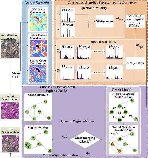
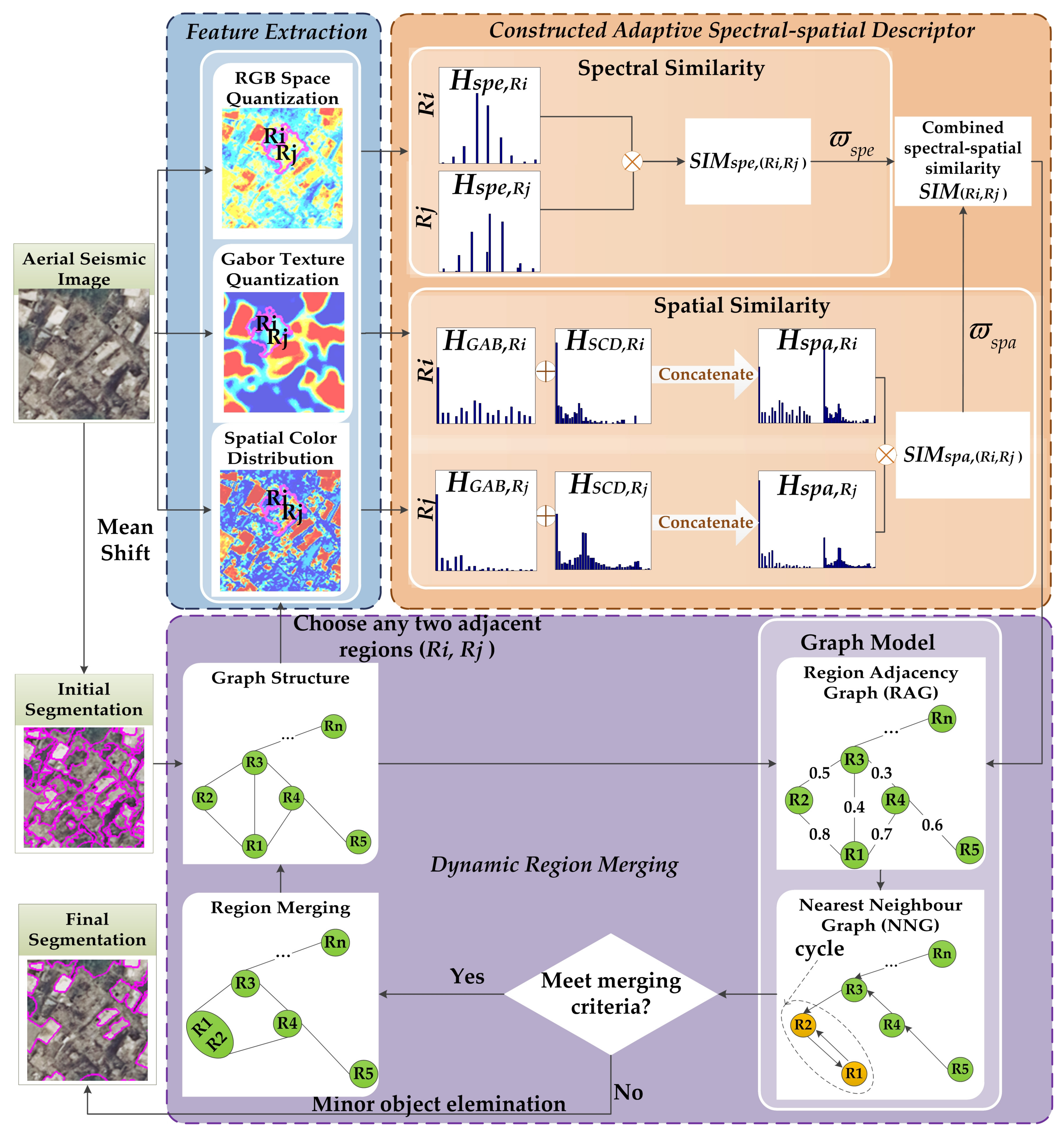
2.1. Feature Extraction and Adaptive Spectral-Spatial Descriptor
2.1.1. Feature Extraction
2.1.2. Adaptive Spectral-Spatial Descriptor
2.2. Dynamic Region Merging Based on Graph Models
- (1)
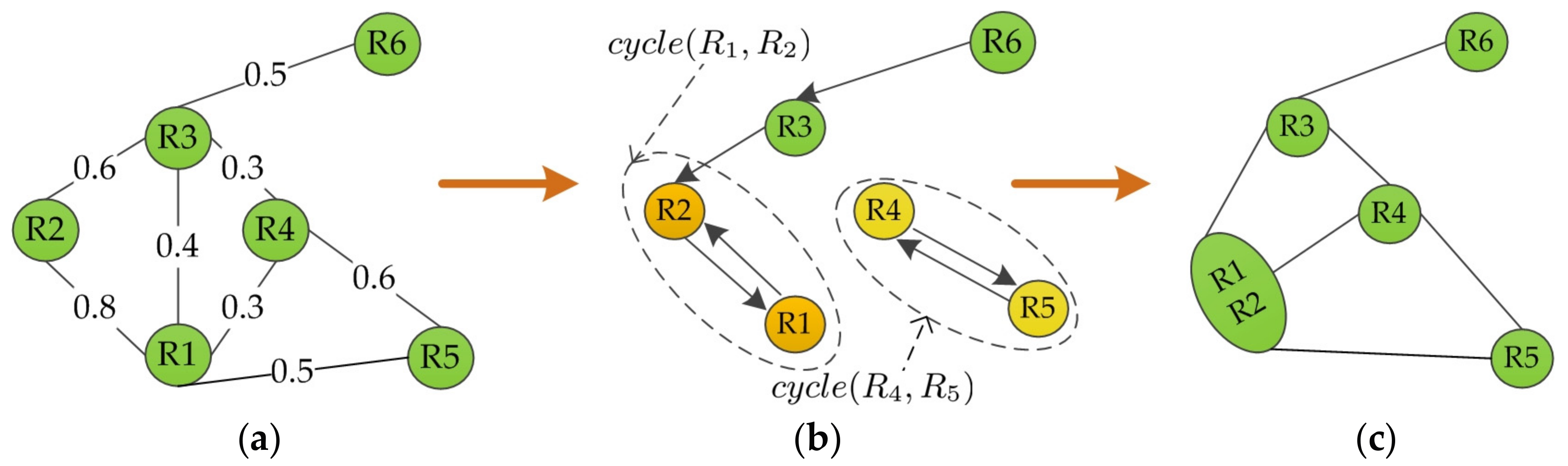
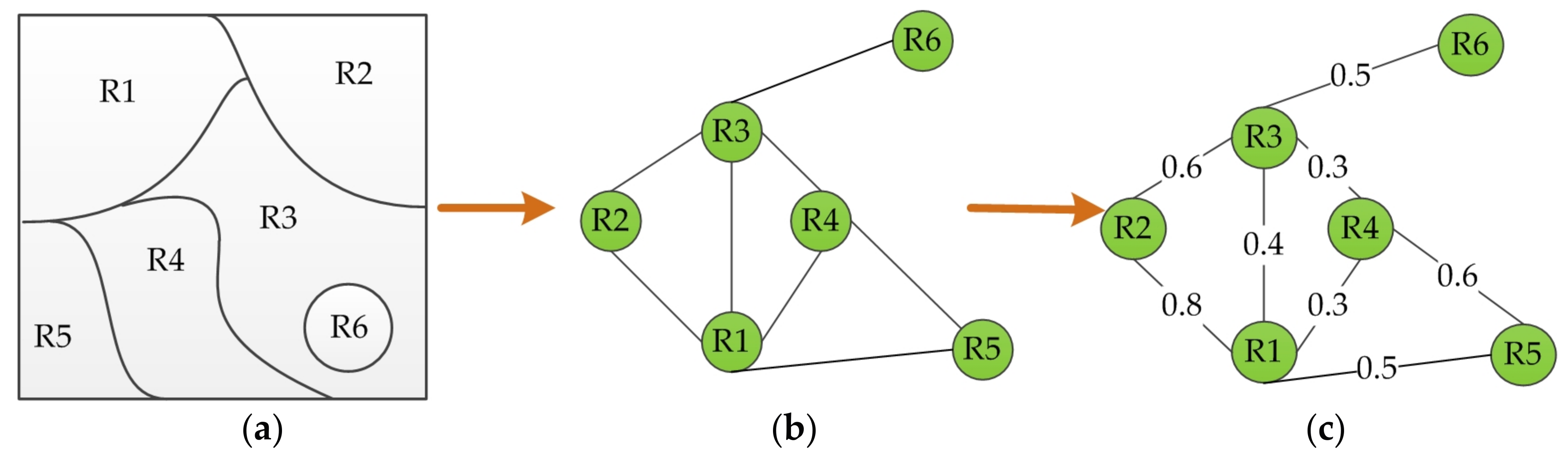
- Graph structure construction. The graph structure of a segmented image is defined as , where V is a set of nodes corresponding to regions, and any two adjacent or neighboring nodes are connected with an edge E. Figure 2a,b shows an example of the constructed graph structure, where Figure 2a is a six-partitioned image and Figure 2b is the corresponding graph structure. As can be seen in Figure 2b, the edges of graph structure here express only the topology of the graph nodes without the similarity information.
- (2)
- Region adjacency graph (RAG). In order to guide the subsequent region merging, the similarity between any two adjacent regions ( ) is required. As illustrated in Figure 2c, RAG is formed by assigning a weighted to each graph edge before it is used to guide the region merging process. The calculation of is discussed in Section 2.1.2.
- (3)
- Nearest neighboring graph (NNG) construction. Rather than scanning the whole RAG, region merging is expedited by searching only the priority queue in NNG. The NNG construction consists of three sub-steps [22].Building the directed edges. NNG is defined as a directed graph, where the directed edge starts from one node in RAG and points to its most similar neighboring node (or nodes). The most similar pair of adjacent regions corresponds to the edge with the maximum weight (or weights). This process is illustrated in Figure 3, where for the given RAG in Figure 3a, Figure 3b shows the determined directed edges in NNG. The edge from R1 to R2 has the greatest weight among all edge weights connecting with R1. Therefore, the directed edge from R1 points to R2. The other directed edges are defined similarly.Finding the cycle edges. The cycle edges of NNG are formed when the edges of two nodes point to each other. As demonstrated in Figure 3b, the directed edges of R1 and R2 point to each other, and thus is a cycle edge in NNG. Likewise, is constituted. Note that the global best [35] pair of regions must belong to the region pairs connected by cycle edges. Hence, it is a significant advantage to search among cycle edges for the global best pair since it can reduce the number of candidate pairs significantly.Creating the priority queue. All the cycle edges are recorded in a priority queue sorted by the edge weight, where the edge with the maximum weight is at the top of the priority queue. For example, in Figure 3b the edge weight in is 0.8, which is larger than that 0.6 in , hence the priority queue is (, ).
- (4)
- Region merging. Region merging is conducted according to the priority queue in NNG. For all cycle edges chosen from the priority queue, a threshold is used to decide whether to merge the region pairs or not. Only the cycle edges whose edge weights are larger than are considered for merging. Here measures the similarity of regions, and it ranges from 0 to 1. For example, it is assumed that the threshold is 0.7 to the priority queue (, ) obtained in Figure 3b. As illustrated in Figure 3c, regions are merged in the following process: is on top of the priority queue thus R1 and R2 are first merged on account of the fact that is larger than . On the contrary, although is on the priority queue, R4 and R5 are not merged because is smaller than .
- (5)
- Dynamic iteration. Note that the regions are constantly changing during the merging procedure which consequently requires an updated testing order. Instead of the traditional static way, the ADRM adopts a dynamic strategy. Along the changing regions, the graph structure of region partition is updated accordingly, including the graph models RAG and NNG to find the globally most suitable solution. Correspondingly, the testing order is dynamically adjusted. In this way, region merging will continue until there is no new merging, that is, there is no cycle or no weight of cycle edge larger than in NNG. It is noted that the parameter serves as a scale parameter, which is application-dependent and can be set empirically or interactively.
2.3. Minor Object Elimination
3. Experimental Setup and Results
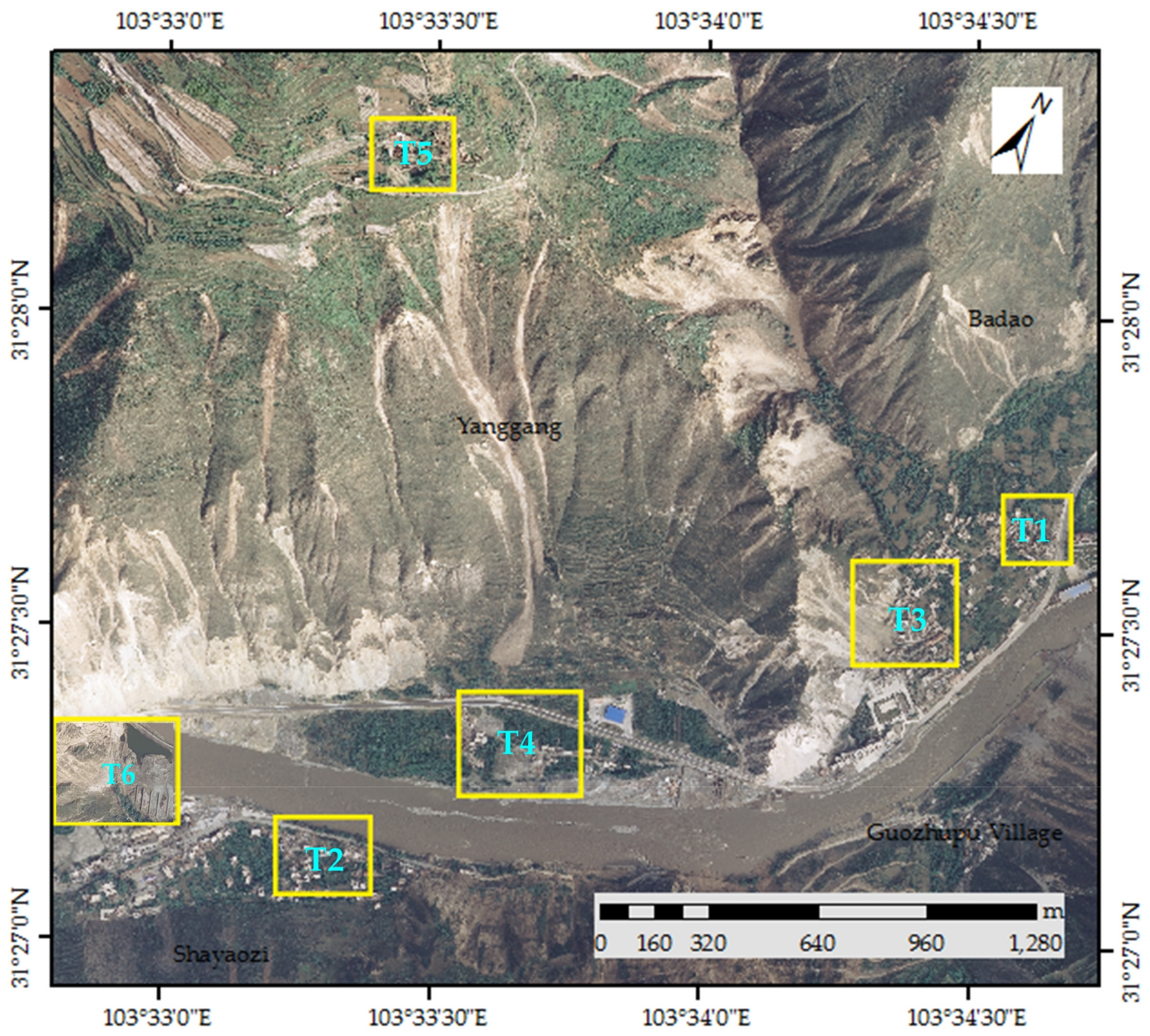
3.1. Data Description
3.2. Evaluation Methods and Metrics
3.3. Comparative Evaluation of Experimental Results
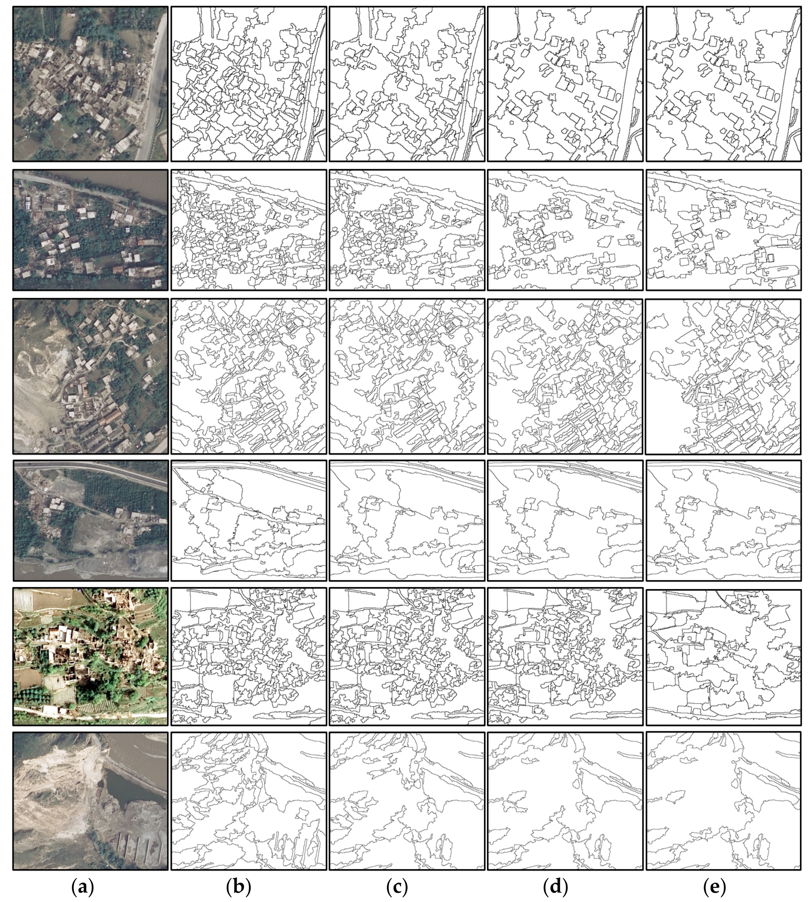
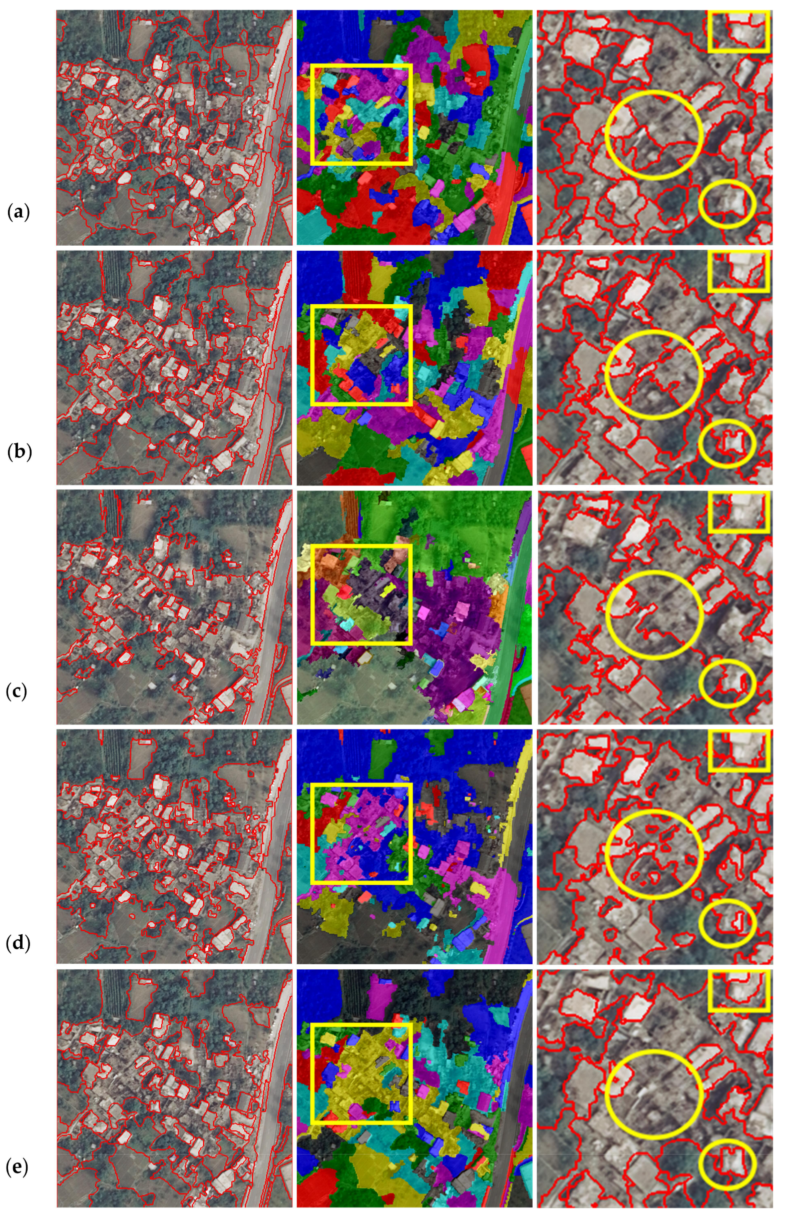
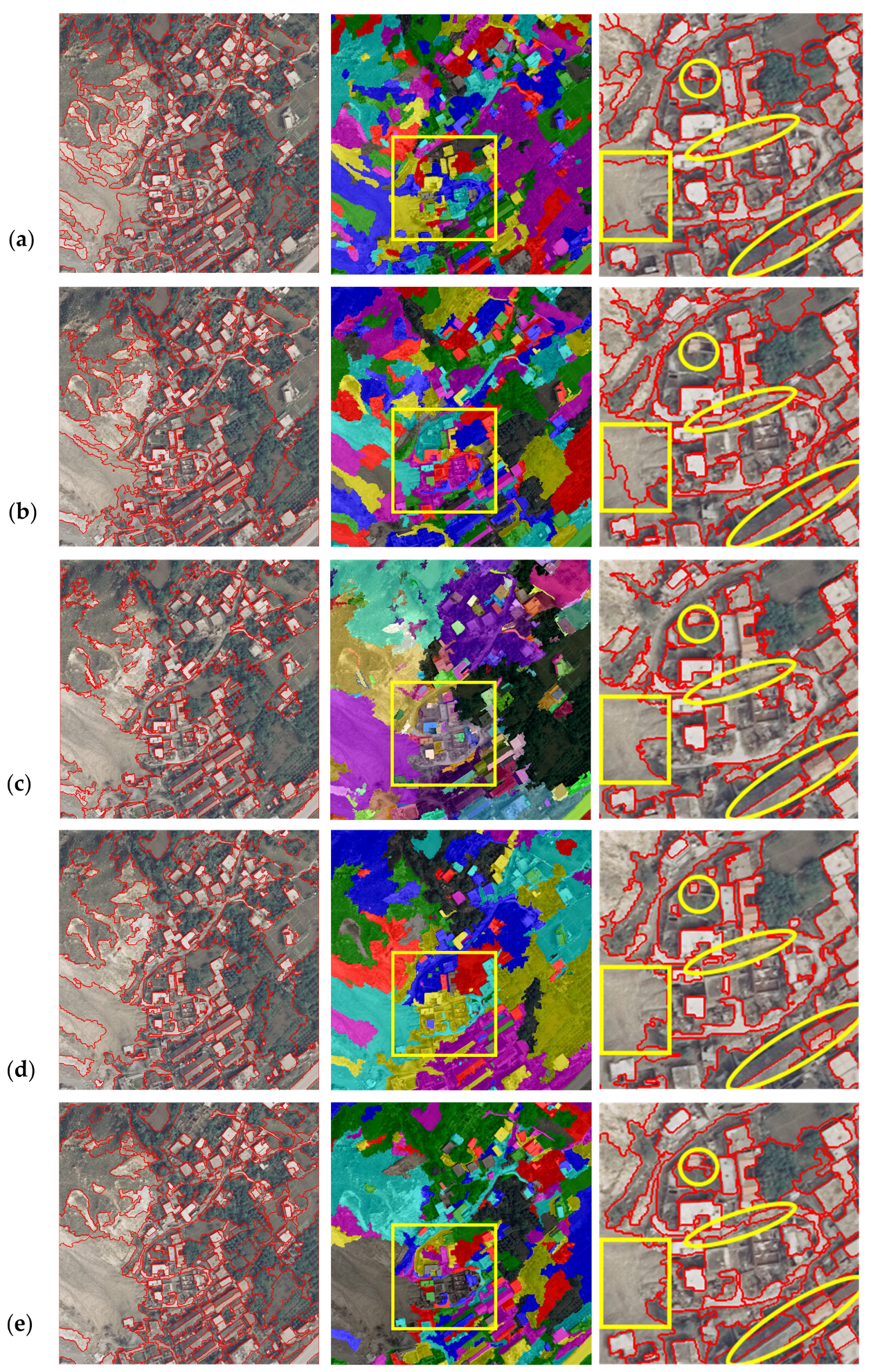
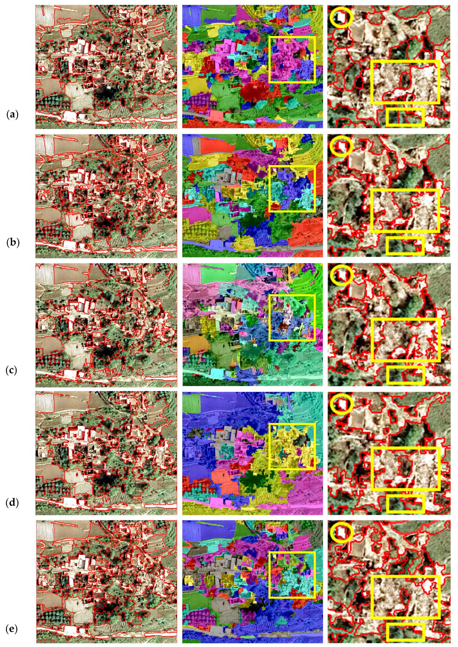
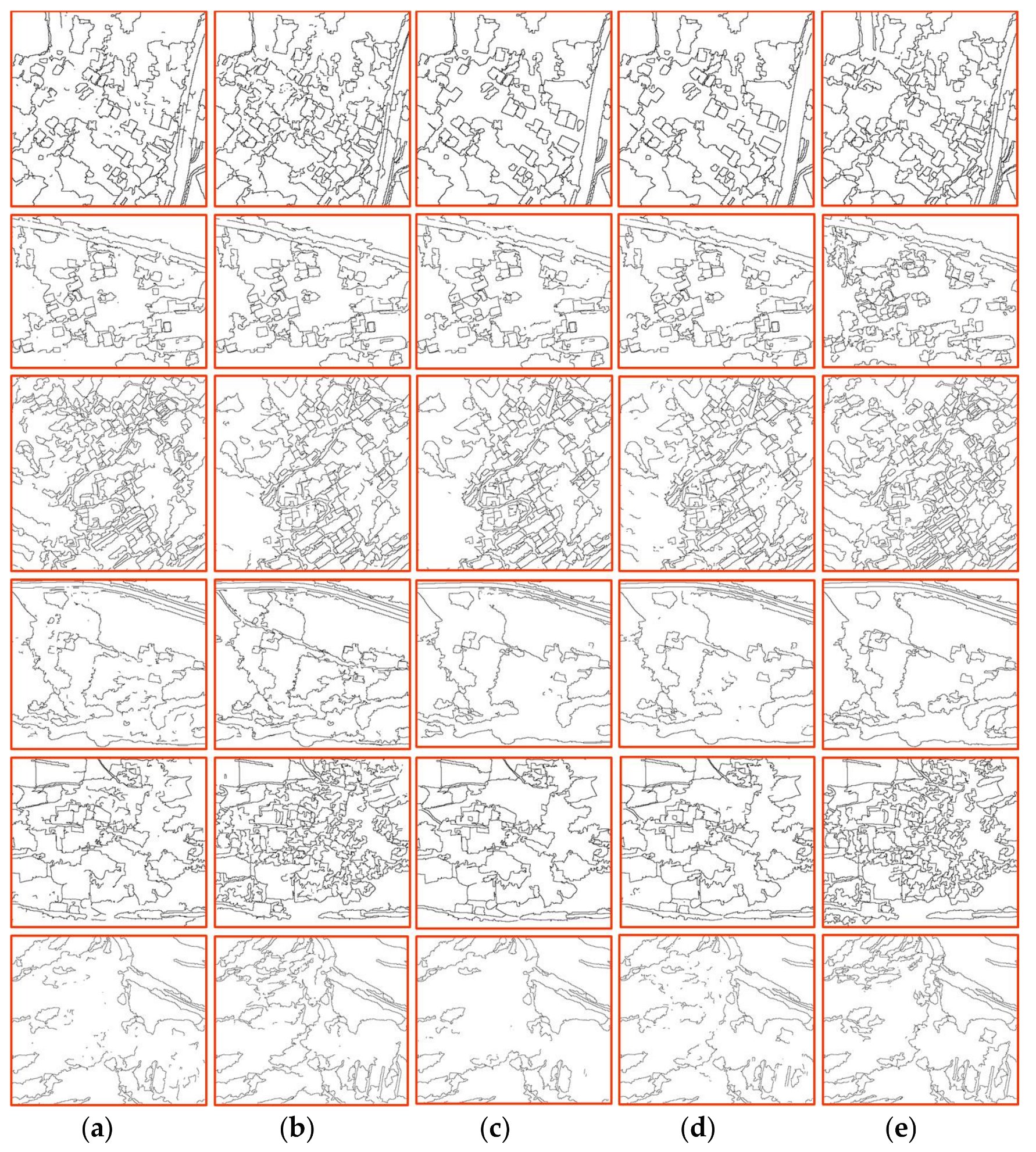
3.3.1. Visual Inspection
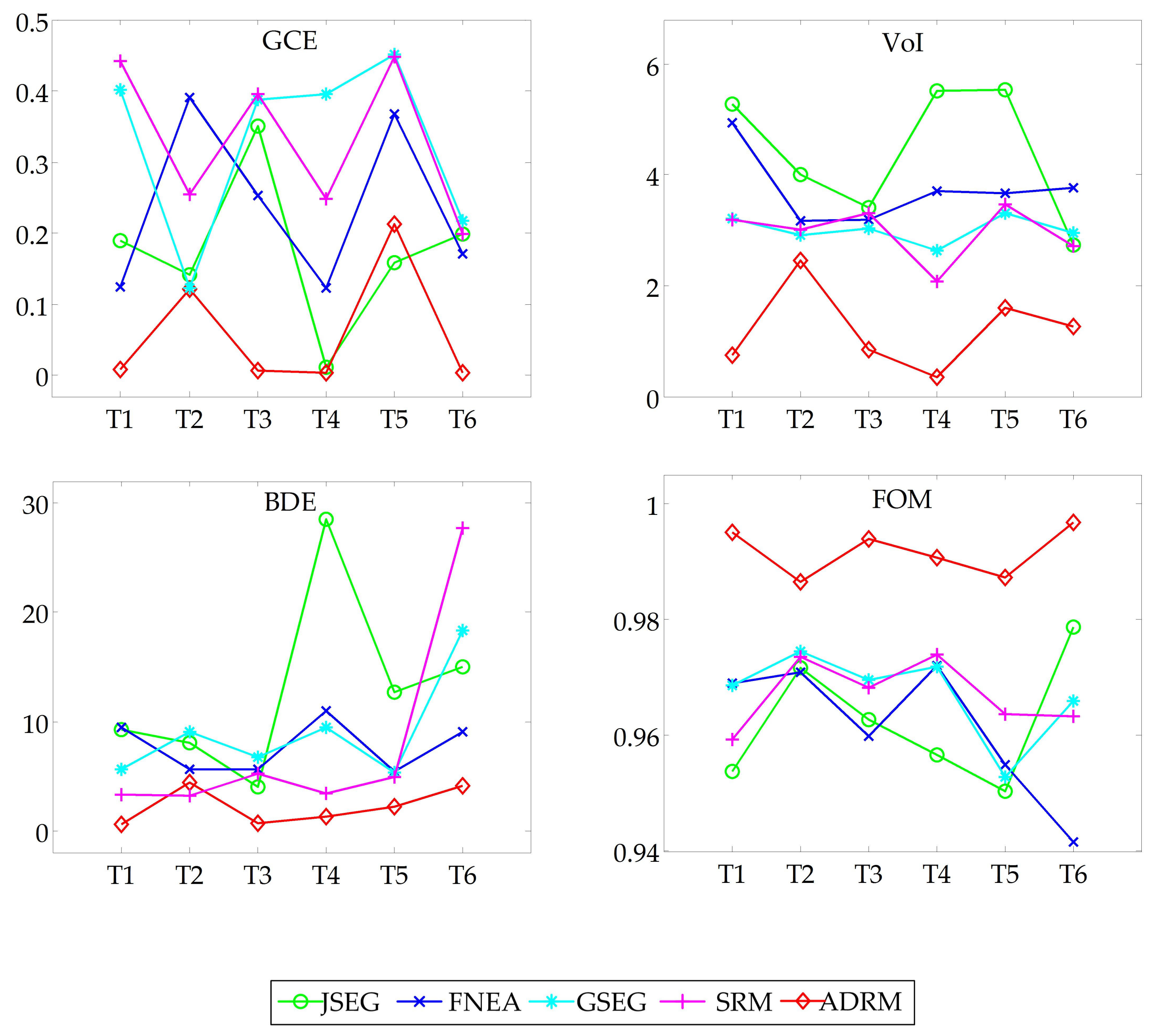
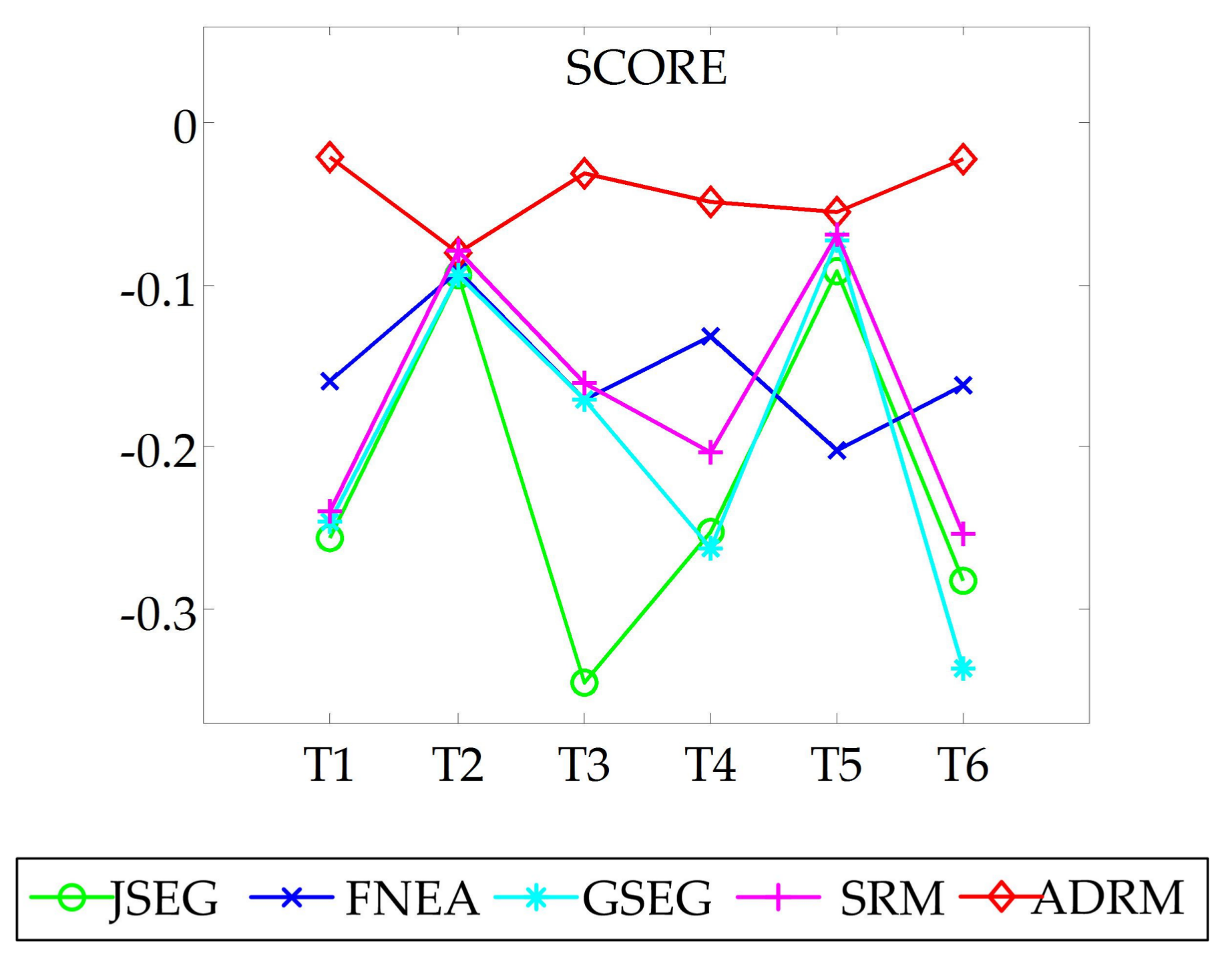
3.3.2. Quantitative Evaluation
3.4. Computational Load Analysis
4. Discussion
5. Conclusions
Acknowledgments
Author Contributions
Conflicts of Interest
References
- Witharana, C.; Civco, D.L.; Meyer, T.H. Evaluation of data fusion and image segmentation in earth observation based rapid mapping workflows. ISPRS J. Photogramm. Remote Sens. 2014, 87, 1–18. [Google Scholar] [CrossRef]
- Nex, F.; Rupnik, E.; Toschi, I.; Remondino, F. Automated processing of high resolution airborne images for earthquake damage assessment. ISPRS Int. Arch. Photogramm. Remote Sens. Spat. Inf. Sci. 2014, 40, 315–321. [Google Scholar] [CrossRef]
- Valero, S.; Chanussot, J.; Benediktsson, J.A.; Talbot, H.; Waske, B. Advanced directional mathematical morphology for the detection of the road network in very high resolution remote sensing images. Pattern Recognit. Lett. 2010, 31, 1120–1127. [Google Scholar] [CrossRef] [Green Version]
- Zhang, Q.; Zhang, Y.; Yang, X.; Su, B. Automatic recognition of seismic intensity based on rs and gis: A case study in Wenchuan ms8.0 earthquake of China. Sci. World J. 2014, 2014, 878149. [Google Scholar] [CrossRef] [PubMed]
- Liu, J.; Li, P.; Wang, X. A new segmentation method for very high resolution imagery using spectral and morphological information. ISPRS J. Photogramm. Remote Sens. 2015, 101, 145–162. [Google Scholar] [CrossRef]
- Yang, J.; He, Y.; Caspersen, J. Region merging using local spectral angle thresholds: A more accurate method for hybrid segmentation of remote sensing images. Remote Sens. Environ. 2017, 190, 137–148. [Google Scholar] [CrossRef]
- Zhao, W.; Du, S. Learning multiscale and deep representations for classifying remotely sensed imagery. ISPRS J. Photogramm. Remote Sens. 2016, 113, 155–165. [Google Scholar] [CrossRef]
- Zhou, C.; Wu, D.; Qin, W.; Liu, C. An efficient two-stage region merging method for interactive image segmentation. Comput. Electr. Eng. 2015, 54, 220–229. [Google Scholar] [CrossRef]
- Ning, J.; Zhang, L.; Zhang, D.; Wu, C. Interactive image segmentation by maximal similarity based region merging. Pattern Recognit. 2010, 43, 445–456. [Google Scholar] [CrossRef]
- Shih, H.C.; Liu, E.R. New quartile-based region merging algorithm for unsupervised image segmentation using color-alone feature. Inf. Sci. 2016, 342, 24–36. [Google Scholar] [CrossRef]
- Yu, Q.; Clausi, D.A. Combining local and global features for image segmentation using iterative classification and region merging. In Proceedings of the Canadian Conference on Computer and Robot Vision, Victoria, BC, Canada, 9–11 May 2005; pp. 579–586. [Google Scholar]
- Crisp, D.J. Improved data structures for fast region merging segmentation using a mumford-shah energy functional. In Proceedings of the Digital Image Computing: Techniques and Applications, Canberra, Australia, 1–3 December 2008; pp. 586–592. [Google Scholar]
- Hu, H.; Liu, H.; Gao, Z.; Huang, L. Hybrid segmentation of left ventricle in cardiac mri using gaussian-mixture model and region restricted dynamic programming. Magn. Reson. Imaging 2012, 31, 575–584. [Google Scholar] [CrossRef] [PubMed]
- Cheng, D.; Meng, G.; Pan, C. Sea-land segmentation via hierarchical region merging and edge directed graph cut. In Proceedings of the IEEE International Conference on Image Processing, Phoenix, AZ, USA, 25–28 August 2016; pp. 1274–1278. [Google Scholar]
- Huang, Z.; Zhang, J.; Li, X.; Zhang, H. Remote sensing image segmentation based on dynamic statistical region merging. Opt. Int. J. Light Electron Opt. 2014, 125, 870–875. [Google Scholar] [CrossRef]
- Gaetano, R.; Masi, G.; Poggi, G.; Verdoliva, L.; Scarpa, G. Marker-controlled watershed-based segmentation of multiresolution remote sensing images. IEEE Trans. Geosci. Remote Sens. 2015, 53, 2987–3004. [Google Scholar] [CrossRef]
- Peng, B.; Zhang, L.; Zhang, D. Automatic image segmentation by dynamic region merging. IEEE Trans. Image Process. 2011, 20, 3592–3605. [Google Scholar] [CrossRef] [PubMed]
- Kailath, T. The divergence and bhattacharyya distance measures in signal selection. IEEE Trans. Commun. Technol. 1967, 15, 52–60. [Google Scholar] [CrossRef]
- Fukunaga, K. Introduction to Statistical Pattern Recognition; Academic Press: San Diego, CA, USA, 1990. [Google Scholar]
- Comaniciu, D.; Ramesh, V.; Meer, P. Kernel-based object tracking. IEEE Trans. Pattern Anal. Mach. Intell. 2003, 25, 564–577. [Google Scholar] [CrossRef]
- Trémeau, A.; Colantoni, P. Regions adjacency graph applied to color image segmentation. IEEE Trans. Image Process. 2000, 9, 735–744. [Google Scholar] [CrossRef] [PubMed]
- Haris, K.; Efstratiadis, S.N.; Maglaveras, N.; Katsaggelos, A.K. Hybrid image segmentation using watersheds and fast region merging. IEEE Trans. Image Process. 1998, 7, 1684–1699. [Google Scholar] [CrossRef] [PubMed]
- Comaniciu, D.; Meer, P. Mean shift: A robust approach toward feature space analysis. IEEE Trans. Pattern Anal. Mach. Intell. 2002, 24, 603–619. [Google Scholar] [CrossRef]
- Kumar, A.; Kumar, P.; Hod, P. A new framework for color image segmentation using watershed algorithm. Comput. Eng. Intell. Syst. 2011, 2, 41–46. [Google Scholar]
- Sumengen, B. Variational Image Segmentation and Curve Evolution on Natural Images. Ph.D. Thesis, University of California, Santa Barbara, CA, USA, 2004. [Google Scholar]
- Bhagavathy, S.; Manjunath, B.S. Modeling and detection of geospatial objects using texture motifs. IEEE Trans. Geosci. Remote Sens. 2005, 44, 3706–3715. [Google Scholar] [CrossRef]
- Kiranyaz, S.; Birinci, M.; Gabbouj, M. Perceptual color descriptor based on spatial distribution: A top-down approach. Image Vis. Comput. 2010, 28, 1309–1326. [Google Scholar] [CrossRef]
- Chapelle, O.; Haffner, P.; Vapnik, V. Svms for histogram-based image classification. IEEE Trans. Neural Netw. 1999, 10, 1055–1064. [Google Scholar] [CrossRef] [PubMed]
- Yang, M.; Zhang, L.; Shiu, C.K.; Zhang, D. Monogenic binary coding: An efficient local feature extraction approach to face recognition. IEEE Trans. Inf. Forensics Secur. 2012, 7, 1738–1751. [Google Scholar] [CrossRef]
- Yuan, J.; Wang, D.L.; Li, R. Remote sensing image segmentation by combining spectral and texture features. IEEE Trans. Geosci. Remote Sens. 2014, 52, 16–24. [Google Scholar] [CrossRef]
- Abdi, H.; Williams, L.J. Principal component analysis. Wiley Interdiscip. Rev. Comput. Stat. 2010, 2, 433–459. [Google Scholar] [CrossRef]
- Reynolds, D. Gaussian mixture models. In Encyclopedia of Biometrics; Li, S.Z., Jain, A., Eds.; Springer: Boston, MA, USA, 2009; pp. 659–663. [Google Scholar]
- Hu, Z.; Wu, Z.; Zhang, Q.; Fan, Q.; Xu, J. A spatially-constrained color-texture model for hierarchical vhr image segmentation. IEEE Geosci. Remote Sens. Lett. 2013, 10, 120–124. [Google Scholar] [CrossRef]
- Liang, L.; Ning, S.; Kai, W.; Yan, G. Change detection method for remote sensing images based on multi-features fusion. Acta Geod. Cartogr. Sin. 2014, 43, 945–953. [Google Scholar]
- Chen, B.; Qiu, F.; Wu, B.; Du, H. Image segmentation based on constrained spectral variance difference and edge penalty. Remote Sens. 2015, 7, 5980–6004. [Google Scholar] [CrossRef]
- Baatz, M.; Schäpe, A. Multiresolution segmentation: An optimization approach for high quality multi-scale image segmentation. In Angewandte Geographische Informationsverarbeitung XII; Strobl, J., Blaschke, T., Griesebner, G., Eds.; Wichmann: Karlsruhe, Germany, 2000; pp. 12–23. [Google Scholar]
- Richard, N.; Frank, N. Statistical region merging. IEEE Trans. Pattern Anal. Mach. Intell. 2004, 26, 1452–1458. [Google Scholar]
- Deng, Y.; Manjunath, B. Unsupervised segmentation of color-texture regions in images and video. IEEE Trans. Pattern Anal. Mach. Intell. 2001, 23, 800–810. [Google Scholar] [CrossRef]
- Felzenszwalb, P.F.; Huttenlocher, D.P. Efficient graph-based image segmentation. Int. J. Comput. Vis. 2004, 59, 167–181. [Google Scholar] [CrossRef]
- Hay, G.J.; Blaschke, T.; Marceau, D.J.; Bouchard, A. A comparison of three image-object methods for the multiscale analysis of landscape structure. ISPRS J. Photogramm. Remote Sens. 2003, 57, 327–345. [Google Scholar] [CrossRef]
- Lang, F.; Yang, J.; Li, D.; Zhao, L.; Shi, L. Polarimetric sar image segmentation using statistical region merging. IEEE Geosci. Remote Sens. Lett. 2014, 11, 509–513. [Google Scholar] [CrossRef]
- Benz, U.C.; Hofmann, P.; Willhauck, G.; Lingenfelder, I.; Heynen, M. Multi-resolution, object-oriented fuzzy analysis of remote sensing data for gis-ready information. ISPRS J. Photogramm. Remote Sens. 2004, 58, 239–258. [Google Scholar] [CrossRef]
- Drăguţ, L.; Csillik, O.; Eisank, C.; Tiede, D. Automated parameterisation for multi-scale image segmentation on multiple layers. ISPRS J. Photogramm. Remote Sens. 2014, 88, 119–127. [Google Scholar] [CrossRef] [PubMed]
- Drǎguţ, L.; Tiede, D.; Levick, S.R. Esp: A tool to estimate scale parameter for multiresolution image segmentation of remotely sensed data. Int. J. Geogr. Inf. Sci. 2010, 24, 859–871. [Google Scholar] [CrossRef]
- Peng, B.; Zhang, L. Evaluation of Image Segmentation Quality by Adaptive Ground Truth Composition; Springer: Berlin/Heidelberg, Germany, 2012. [Google Scholar]
- Meilă, M. Comparing clusterings—An information based distance. J. Multivar. Anal. 2007, 98, 873–895. [Google Scholar] [CrossRef]
- Martin, D.; Fowlkes, C.; Tal, D.; Malik, J. A database of human segmented natural images and its application to evaluating segmentation algorithms and measuring ecological statistics. In Proceedings of the Eighth IEEE International Conference on Computer Vision, Vancouver, BC, Canada, 7–14 July 2001; Volume 412, pp. 416–423. [Google Scholar]
- Freixenet, J.; Muñoz, X.; Raba, D.; Martí, J.; Cufí, X. Yet another survey on image segmentation: Region and boundary information integration. In Computer Vision—ECCV 2002; Heyden, A., Sparr, G., Nielsen, M., Johansen, P., Eds.; Springer: Berlin/Heidelberg, Germany, 2002; Volume 2352, pp. 408–422. [Google Scholar]


| Image | Platform | Size (Pixel) | Resolution | Landscape |
|---|---|---|---|---|
| T1 | Aerial | 400 × 400 | 0.67 m | Rural collapsed residential area, forest, road |
| T2 | Aerial | 510 × 404 | 0.67 m | Rural collapsed residential area, debris flow, forest |
| T3 | Aerial | 600 × 600 | 0.67 m | Landslide, collapsed residential area, forest, road |
| T4 | Aerial | 556 × 474 | 0.67 m | Rural collapsed residential area and debris flow |
| T5 | Aerial | 475 × 416 | 0.67 m | Rural collapsed residential area, forest farmland |
| T6 | Aerial | 700 × 596 | 0.67 m | Debris flow, landslide |
| Methods | Parameters | T1 | T2 | T3 | T4 | T5 | T6 |
|---|---|---|---|---|---|---|---|
| ADRM | 0.86 | 0.83 | 0.88 | 0.83 | 0.84 | 0.85 | |
| JSEG | Nu | 153 | 104 | 305 | 127 | 207 | 63 |
| FNEA | scale | 53 | 54 | 56 | 50 | 58 | 41 |
| SRM | 1 | 4 | 4 | 8 | 16 | 4 | |
| GSEG | K | 400 | 500 | 400 | 500 | 600 | 400 |
| Metric | What Measures |
|---|---|
| VoI | The VoI defines the distance between two segmentations as average conditional entropy of one segmentation given by the other segmentation, and thus measures the amount of randomness in one segmentation which cannot be explained by the other. The VoI metric is non-negative, with lower values indicating greater similarity. |
| GCE | The GCE measures the extent to which one segmentation can be viewed as a refinement of the other. Segmentations which are related in this manner are considered to be consistent, since they can represent the same natural image segmented at different scales. |
| BDE | The BDE measures the average displacement error of boundary pixels between two segmented images. Particularly, it defines the error of one boundary pixel as the distance between the pixel and the closest boundary pixel in the other image. |
| FOM | The Pratt figure of merit (FOM) corresponds to a measure of the global behavior of the distance between a segmentation and its reference segmentation; and it is a relative measure that varies in the interval [0, 1]. |
| Metrics | Methods | Images | |||||||
|---|---|---|---|---|---|---|---|---|---|
| T1 | T2 | T3 | T4 | T5 | T6 | Mean | Var | ||
| GCE | JSEG | 0.189 | 0.141 | 0.351 | 0.010 | 0.158 | 0.199 | 0.175 | 0.012 |
| FNEA | 0.125 | 0.39 | 0.252 | 0.122 | 0.367 | 0.171 | 0.238 | 0.012 | |
| GSEG | 0.402 | 0.122 | 0.388 | 0.396 | 0.451 | 0.217 | 0.329 | 0.014 | |
| SRM | 0.442 | 0.254 | 0.395 | 0.248 | 0.448 | 0.198 | 0.331 | 0.010 | |
| ADRM | 0.008 | 0.122 | 0.006 | 0.004 | 0.213 | 0.004 | 0.060 | 0.008 | |
| VoI | JSEG | 5.289 | 4.015 | 3.413 | 5.515 | 5.535 | 2.742 | 4.418 | 1.438 |
| FNEA | 4.933 | 3.179 | 3.199 | 3.717 | 3.661 | 3.76 | 3.742 | 0.340 | |
| GSEG | 3.209 | 2.906 | 3.041 | 2.641 | 3.315 | 2.949 | 3.010 | 0.047 | |
| SRM | 3.188 | 3.007 | 3.302 | 2.088 | 3.475 | 2.719 | 2.963 | 0.209 | |
| ADRM | 0.745 | 2.448 | 0.853 | 0.354 | 1.605 | 1.259 | 1.211 | 0.553 | |
| BDE | JSEG | 9.287 | 8.070 | 4.034 | 28.499 | 12.727 | 14.998 | 12.936 | 72.548 |
| FNEA | 9.481 | 5.628 | 5.624 | 10.943 | 5.442 | 9.014 | 7.689 | 4.853 | |
| GSEG | 5.579 | 9.024 | 6.770 | 9.445 | 5.347 | 18.378 | 9.090 | 19.686 | |
| SRM | 3.332 | 3.218 | 5.240 | 3.395 | 4.899 | 27.731 | 7.969 | 78.732 | |
| ADRM | 0.594 | 4.379 | 0.677 | 1.257 | 2.157 | 4.113 | 2.196 | 2.839 | |
| FOM | JSEG | 0.954 | 0.972 | 0.963 | 0.957 | 0.950 | 0.979 | 0.963 | 0.00012 |
| FNEA | 0.969 | 0.971 | 0.960 | 0.972 | 0.955 | 0.942 | 0.961 | 0.00011 | |
| GSEG | 0.969 | 0.974 | 0.970 | 0.972 | 0.953 | 0.966 | 0.967 | 0.00005 | |
| SRM | 0.959 | 0.974 | 0.968 | 0.974 | 0.964 | 0.963 | 0.967 | 0.00003 | |
| ADRM | 0.995 | 0.986 | 0.994 | 0.991 | 0.987 | 0.997 | 0.992 | 0.00002 | |
| Images | JSEG (s) | FNEA (s) | GSEG (s) | SRM (s) | ADRM (s) |
|---|---|---|---|---|---|
| T1 | 2.034 × 10³ | 15.147 | 4.125 | 7.948 | 12.231 |
| T2 | 1.713 × 10³ | 16.131 | 4.344 | 10.209 | 26.771 |
| T3 | 3.362 × 10³ | 53.337 | 4.717 | 13.600 | 32.671 |
| T4 | 2.167 × 10³ | 19.501 | 5.430 | 9.901 | 16.237 |
| T5 | 2.145 × 10³ | 23.619 | 4.538 | 10.644 | 21.511 |
| T6 | 3.249 × 10³ | 26.349 | 4.811 | 13.339 | 21.541 |
| Mean | 2.445 × 10³ | 25.681 | 4.661 | 10.940 | 21.827 |
© 2017 by the authors. Licensee MDPI, Basel, Switzerland. This article is an open access article distributed under the terms and conditions of the Creative Commons Attribution (CC BY) license (http://creativecommons.org/licenses/by/4.0/).
Share and Cite
Sun, G.; Hao, Y.; Chen, X.; Ren, J.; Zhang, A.; Huang, B.; Zhang, Y.; Jia, X. Dynamic Post-Earthquake Image Segmentation with an Adaptive Spectral-Spatial Descriptor. Remote Sens. 2017, 9, 899. https://doi.org/10.3390/rs9090899
Sun G, Hao Y, Chen X, Ren J, Zhang A, Huang B, Zhang Y, Jia X. Dynamic Post-Earthquake Image Segmentation with an Adaptive Spectral-Spatial Descriptor. Remote Sensing. 2017; 9(9):899. https://doi.org/10.3390/rs9090899
Chicago/Turabian StyleSun, Genyun, Yanling Hao, Xiaolin Chen, Jinchang Ren, Aizhu Zhang, Binghu Huang, Yuanzhi Zhang, and Xiuping Jia. 2017. "Dynamic Post-Earthquake Image Segmentation with an Adaptive Spectral-Spatial Descriptor" Remote Sensing 9, no. 9: 899. https://doi.org/10.3390/rs9090899