
Reducing the Effect of the Endmembers’ Spectral Variability by Selecting the Optimal Spectral Bands


Abstract
:
1. Introduction
2. Theoretical Background
2.1. Feature Selection Algorithms to Decrease the Spectral Variability Effect
2.2. Feature Selection Algorithms to Decrease the Spectral Correlation of Endmembers
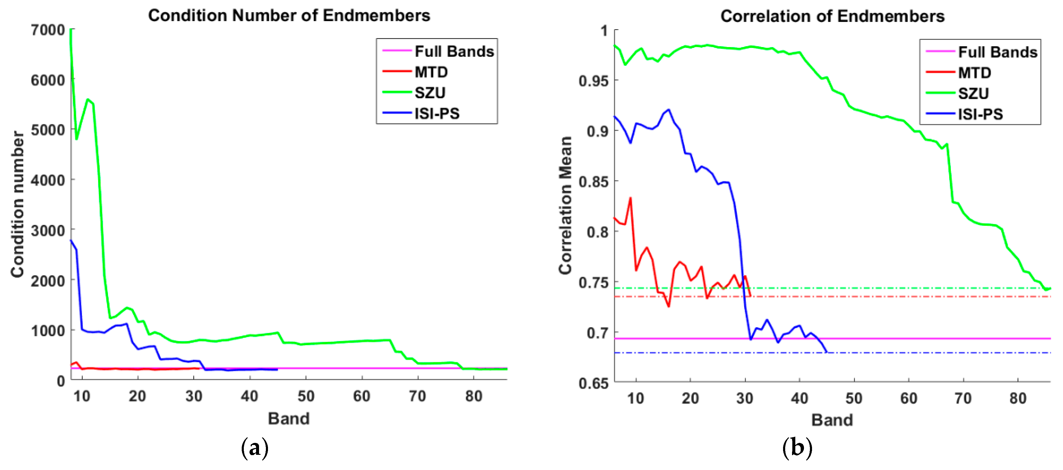
2.2.1. Quantitative Evaluation of the Endmembers’ Correlation
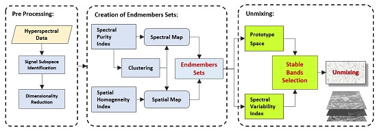
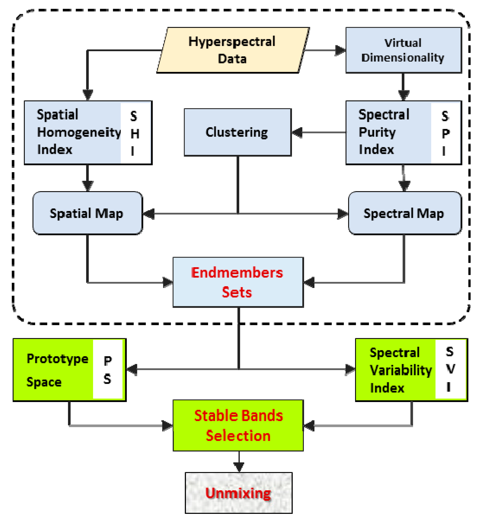
3. The Proposed ISI-PS Method
- (1)
- Estimating the number of classes of the image and establishing a spectral library of the SV of endmembers (i.e., the sets of endmembers).
- (2)
- Prioritizing the persistent bands against the SV using the SV index and some training data.where Ω is the set of prioritized persistent bands (B) and ith is the prioritizing index of bands.
- (3)
- Selecting the most different bands in the PS using the distance of the bands from the main diagonal of the space, .
- (4)
- Considering band and computing its angle from all members of set in the PS.
- (5)
- If the angle of band from all of the previously selected bands was greater than a predefined threshold (T), then ; otherwise, , and band is eliminated.
- (6)
- Unmixing the hyperspectral image using the selected bands.
3.1. Establishing a Set of Spectral Variabilities for Each Endmember
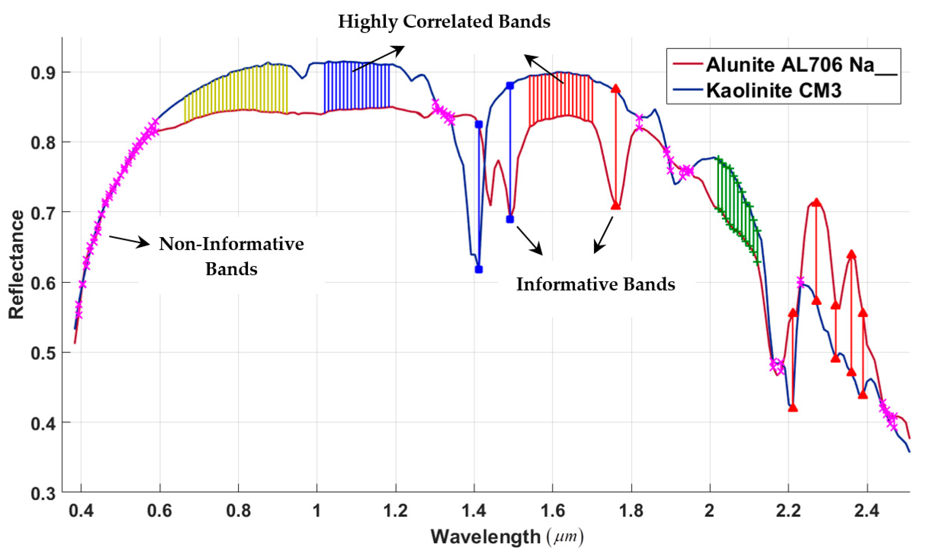
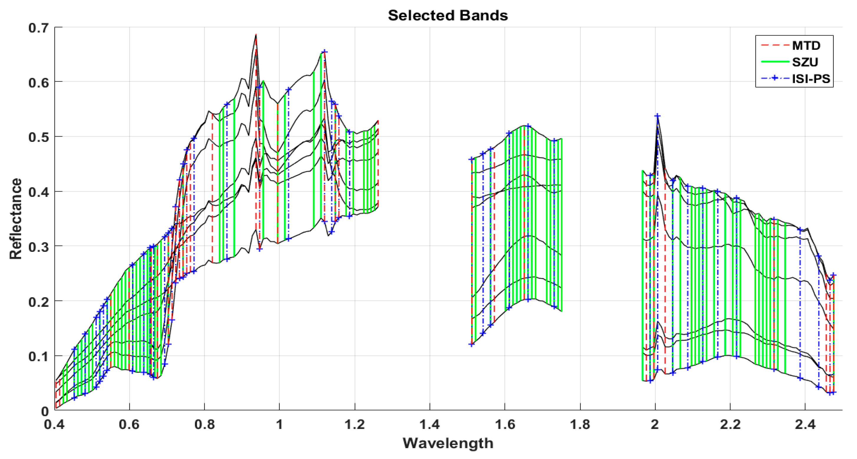
3.2. Reducing the Spectral Variability Effect by Selecting the Optimal Bands
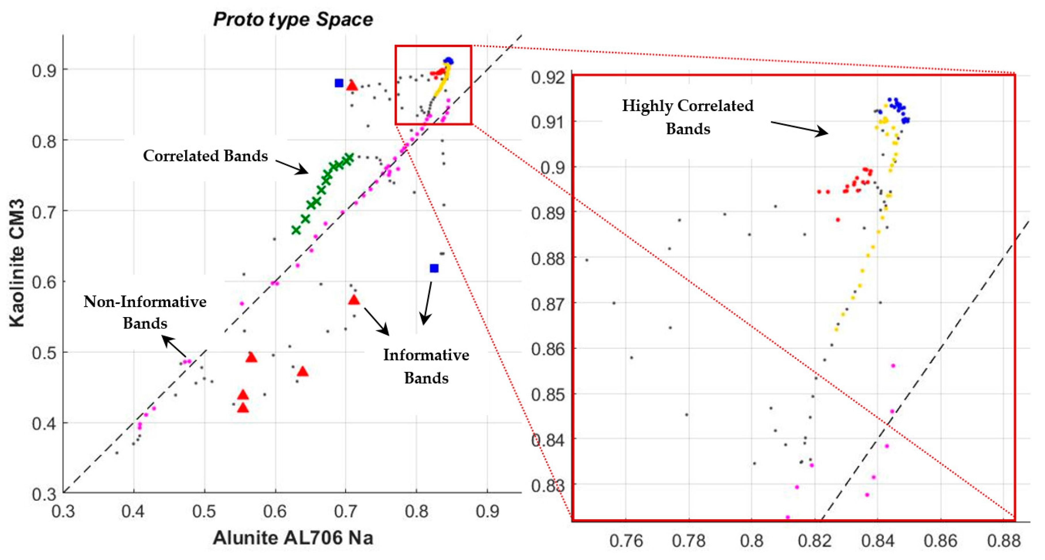
3.3. Reducing the Correlation of Endmembers by Selecting the Independent Bands in the Prototype Space
3.4. Determining the Threshold Value to Identify the Independent Bands
3.5. Spectral Unmixing
4. Results and Discussion
4.1. Simulated and Real Datasets Used
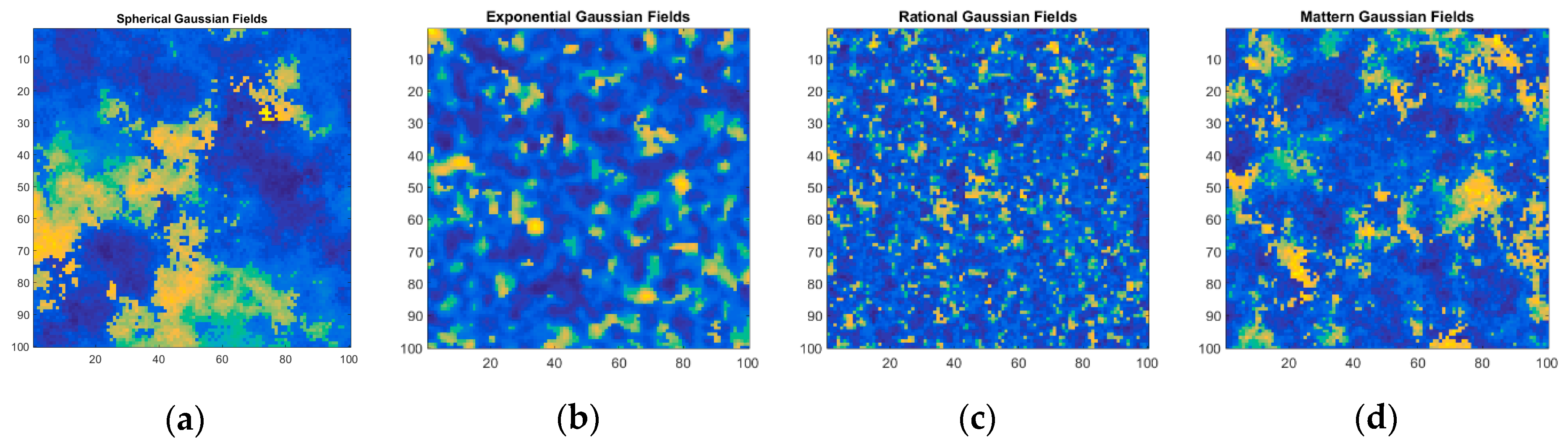
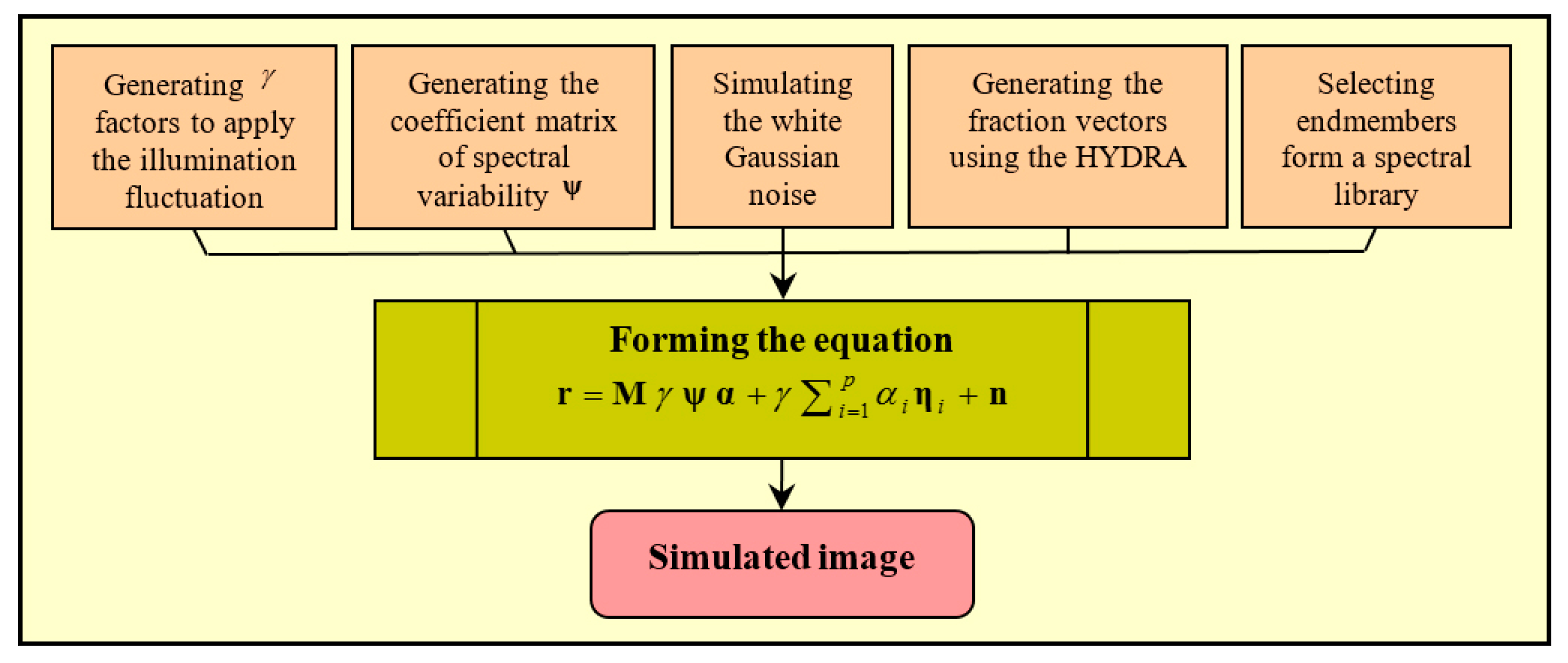
4.1.1. Simulated Dataset
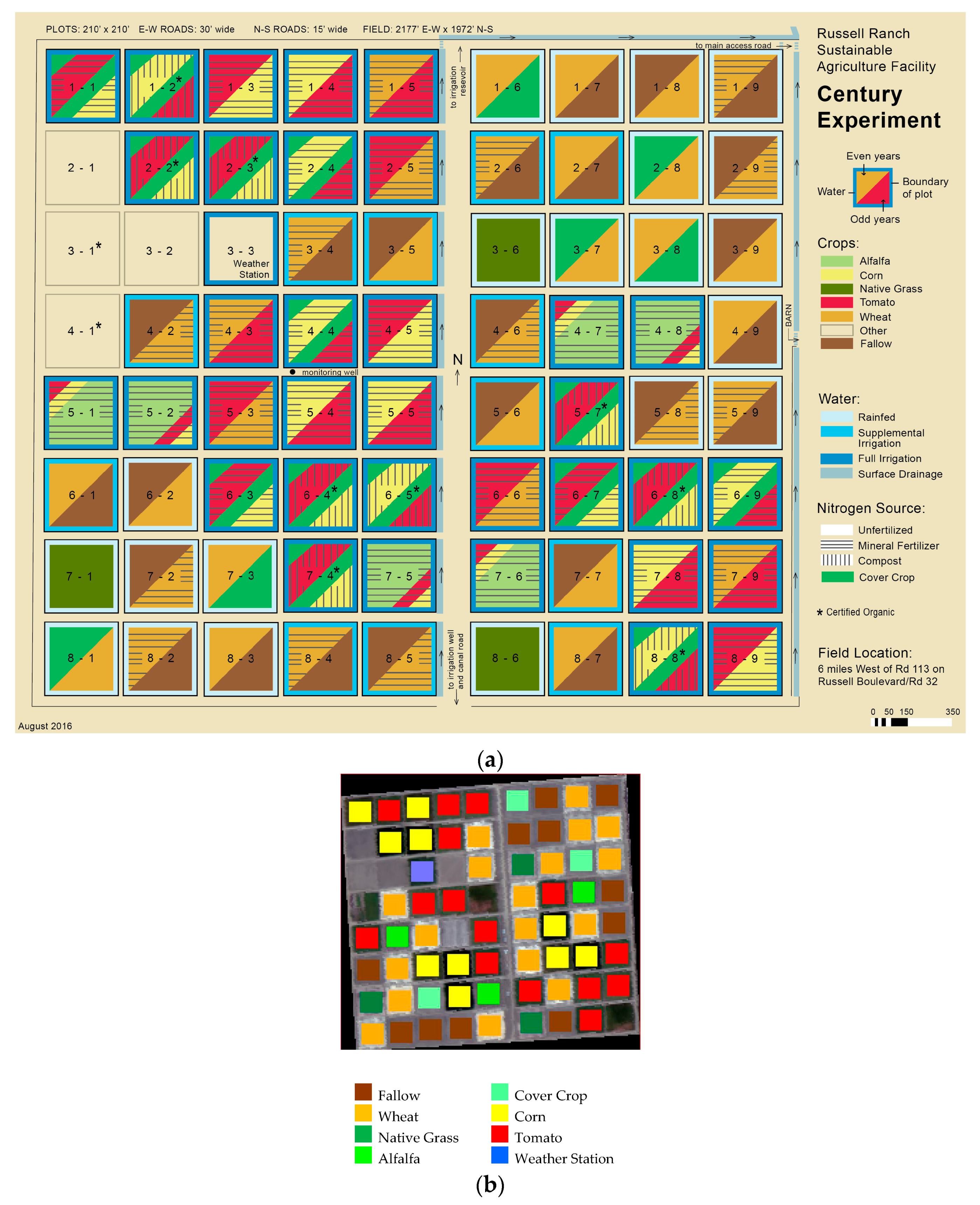
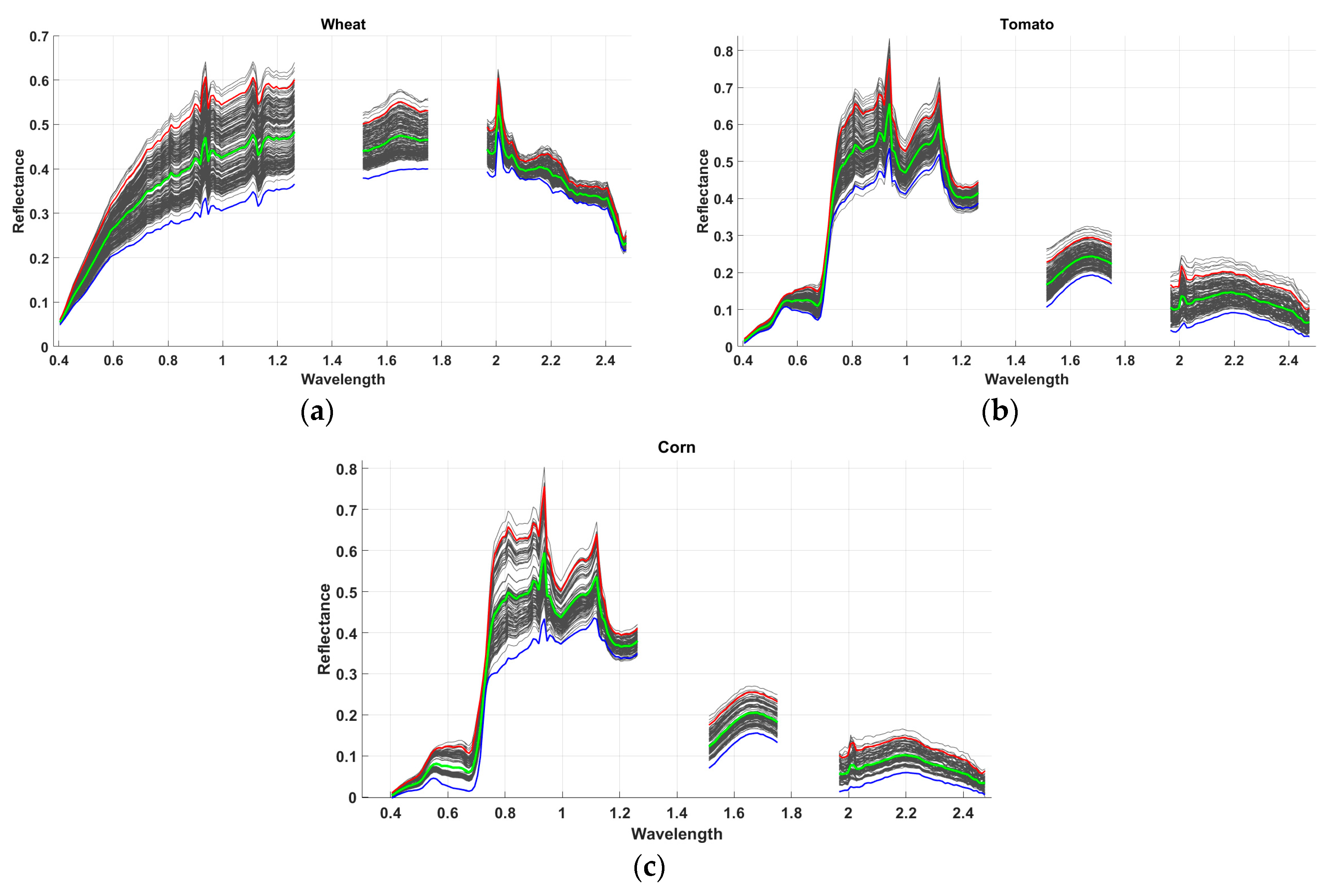
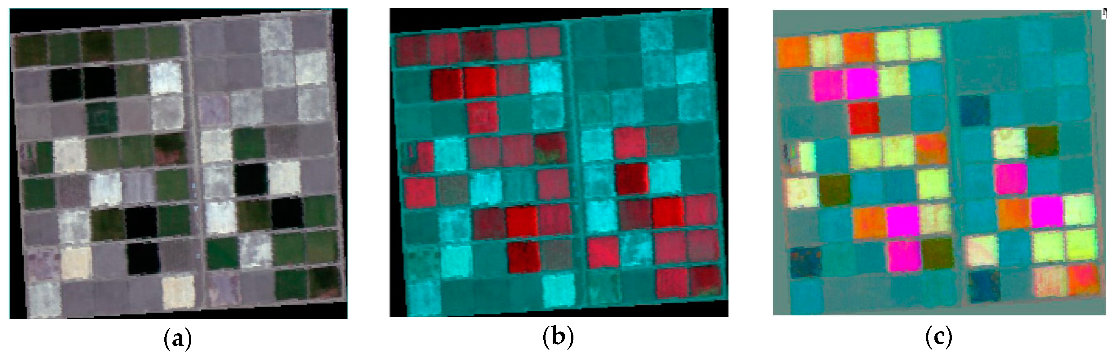
4.1.2. LTRAS Dataset
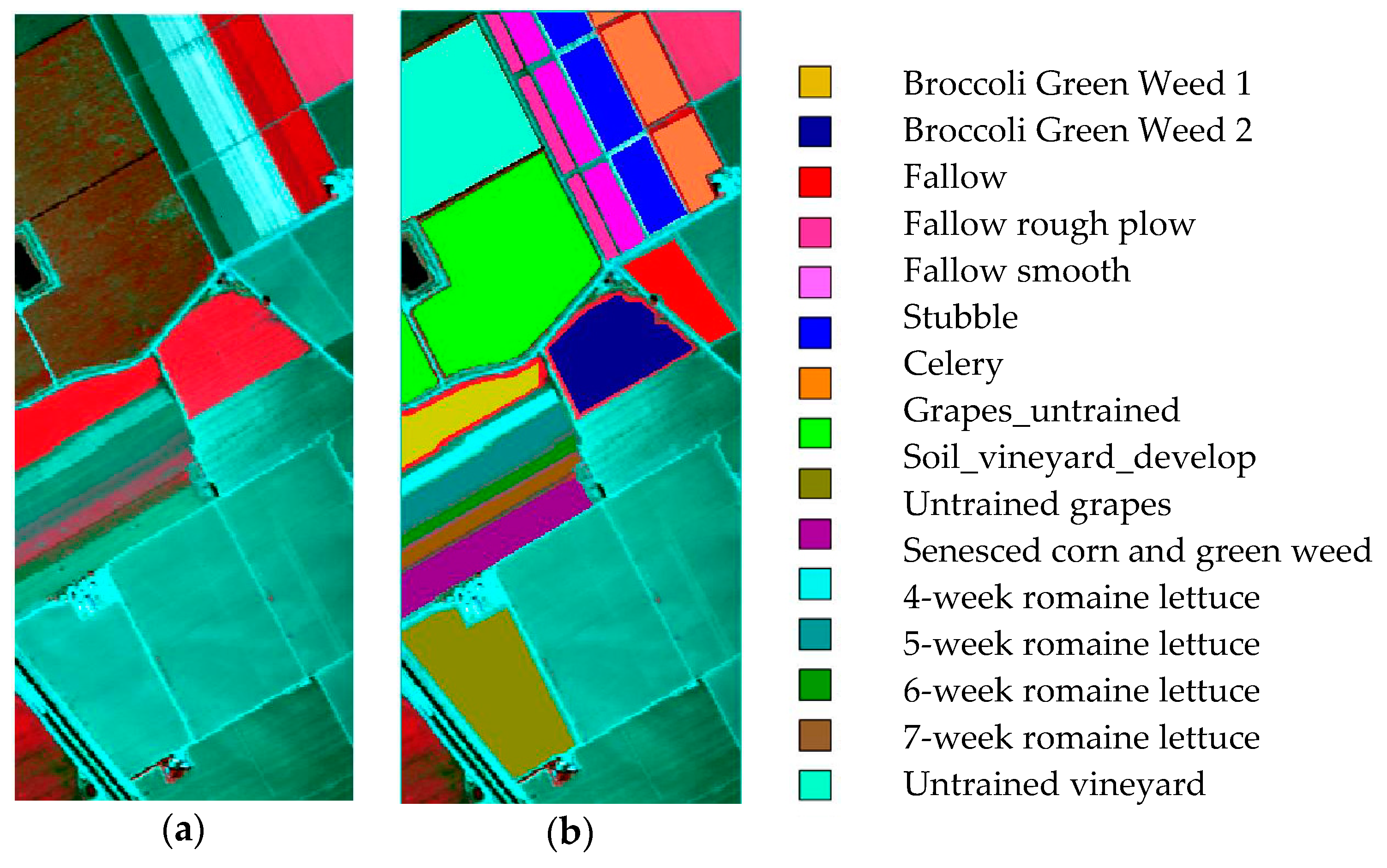
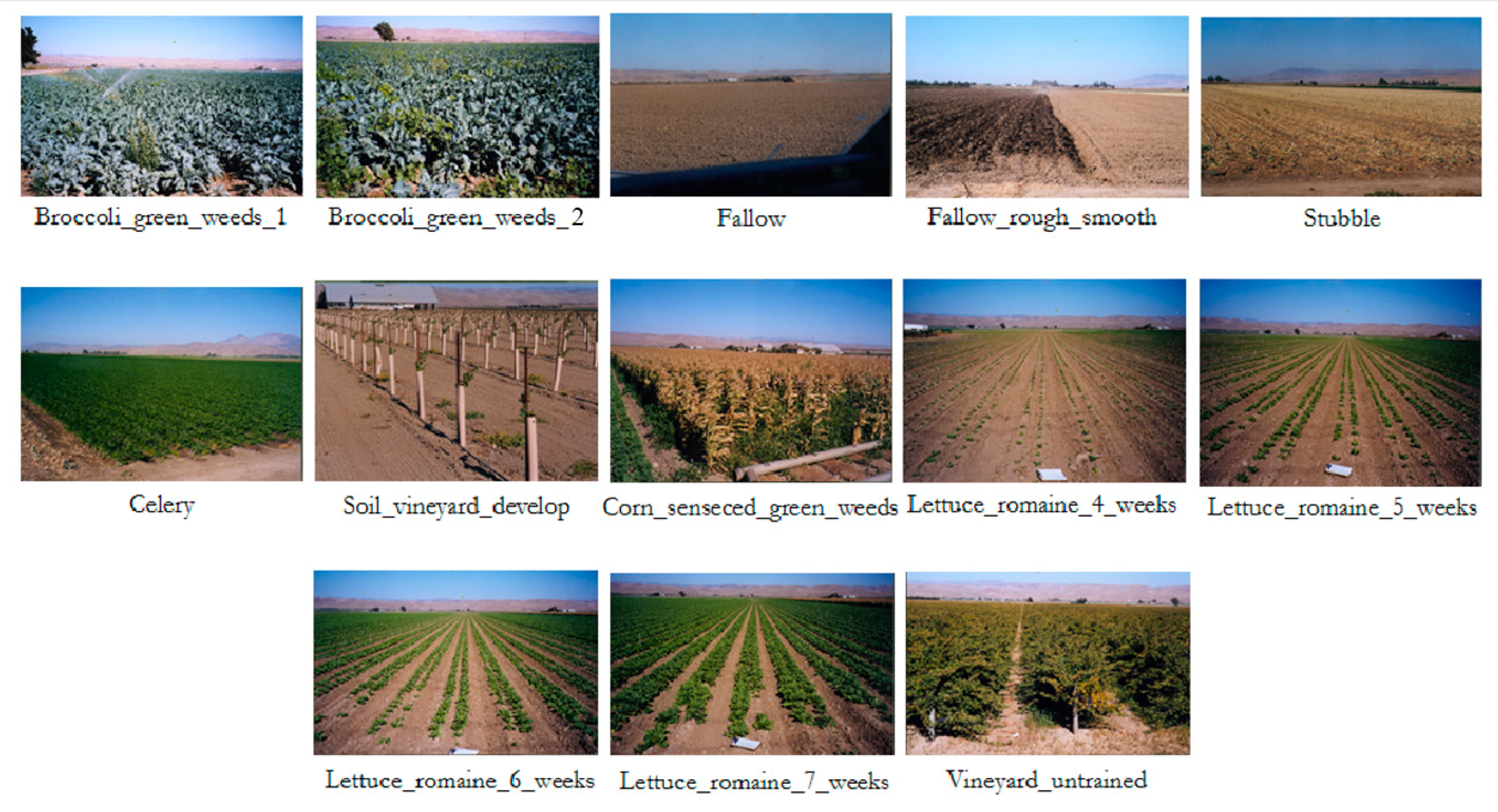
4.1.3. Salinas Dataset
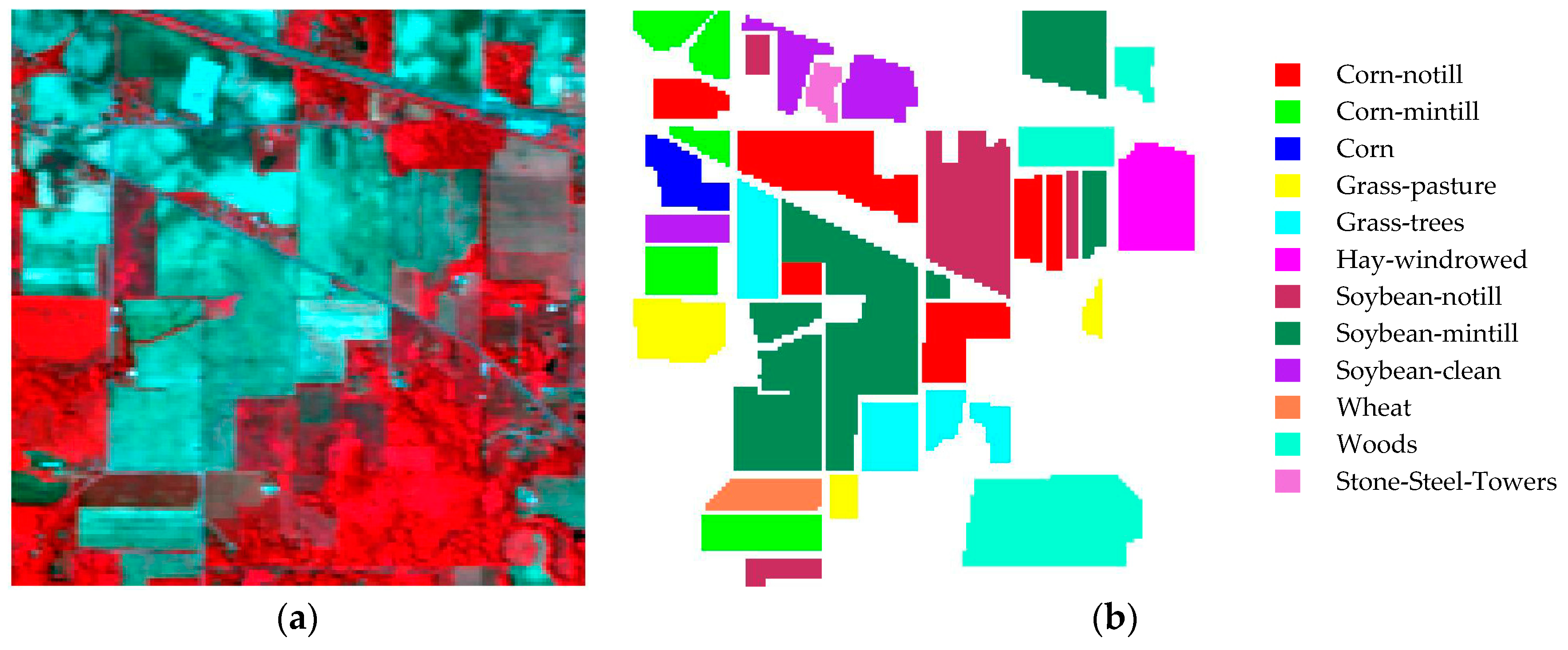
4.1.4. Indiana Indian Pines dataset
4.2. Experiments on the Simulated Dataset
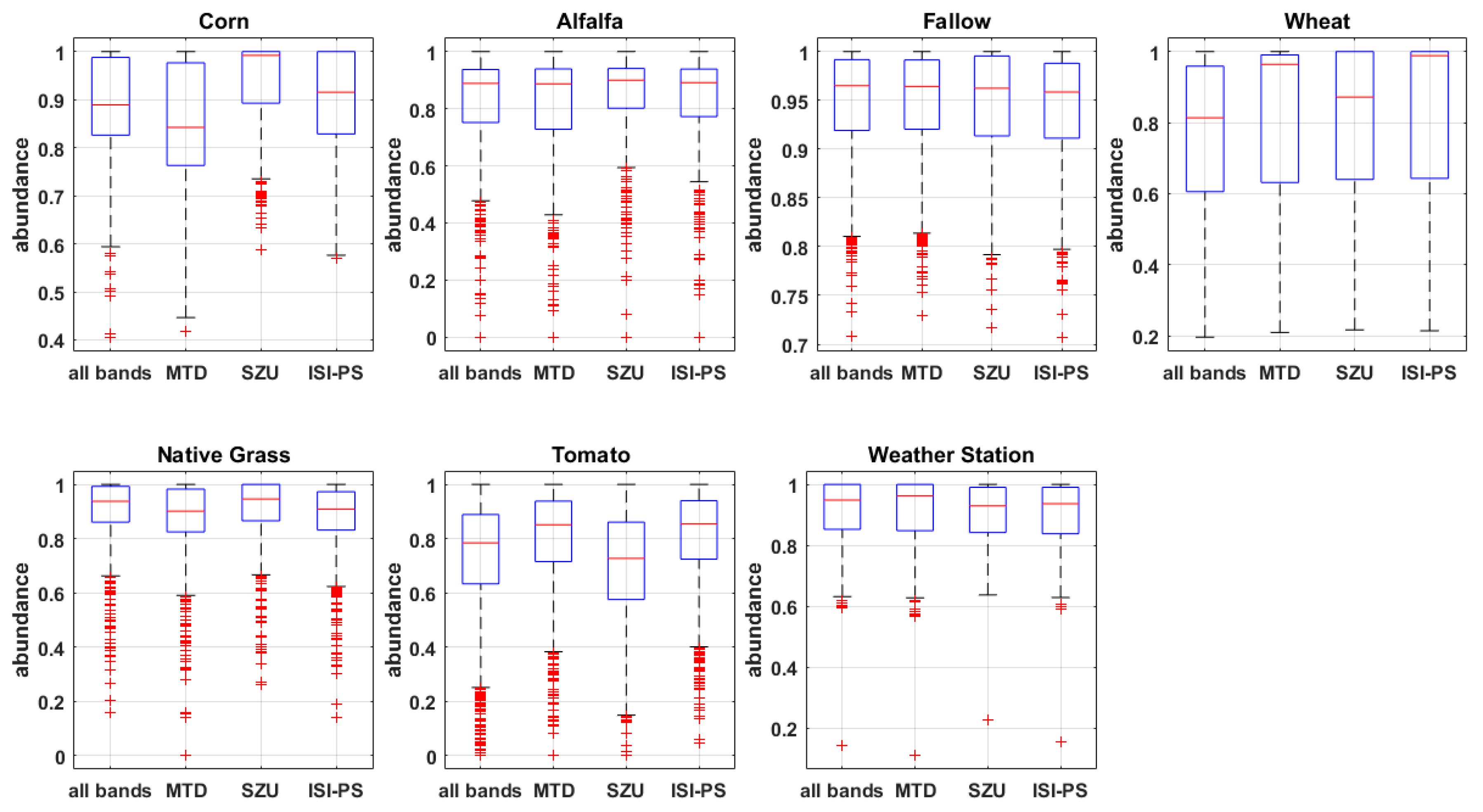
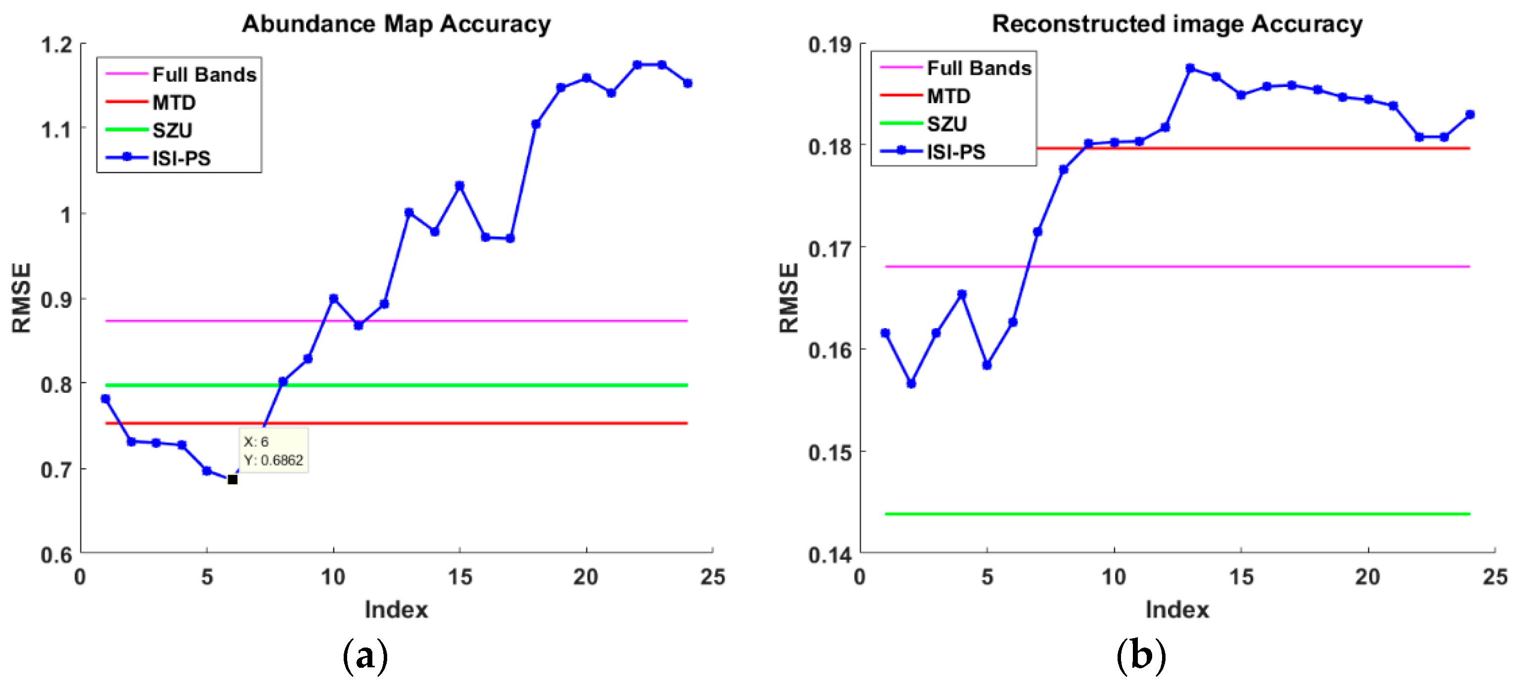
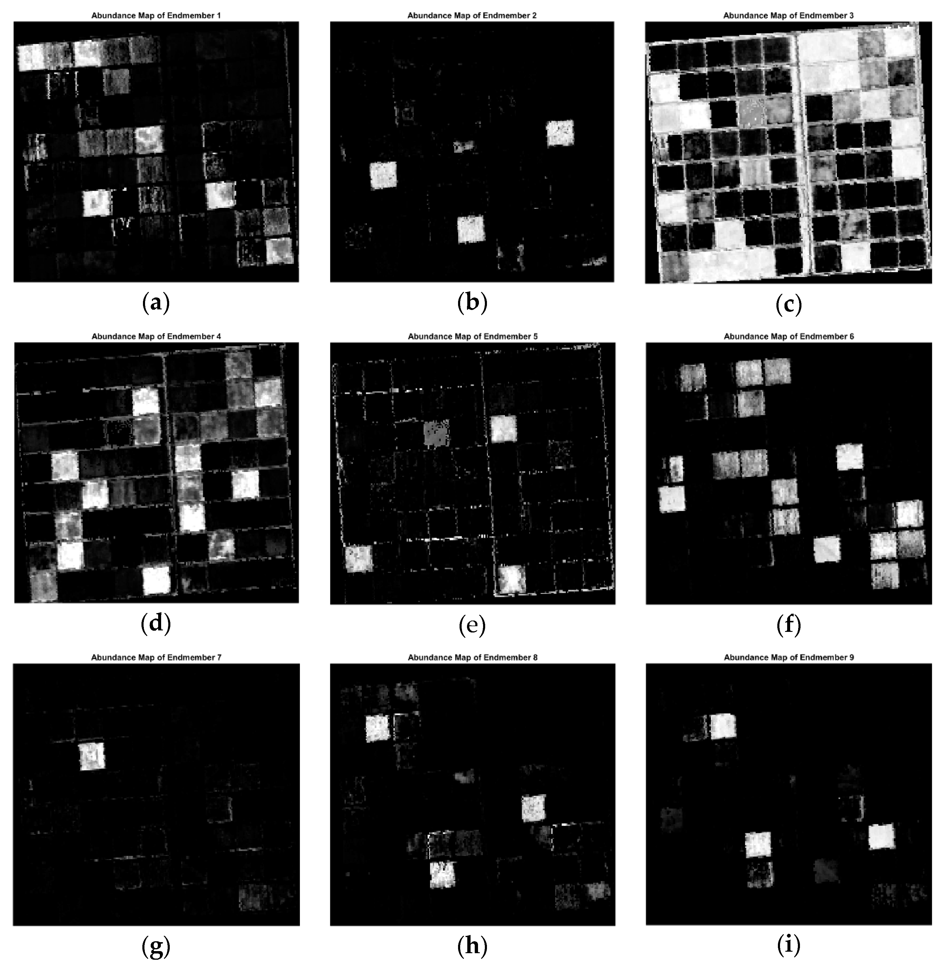
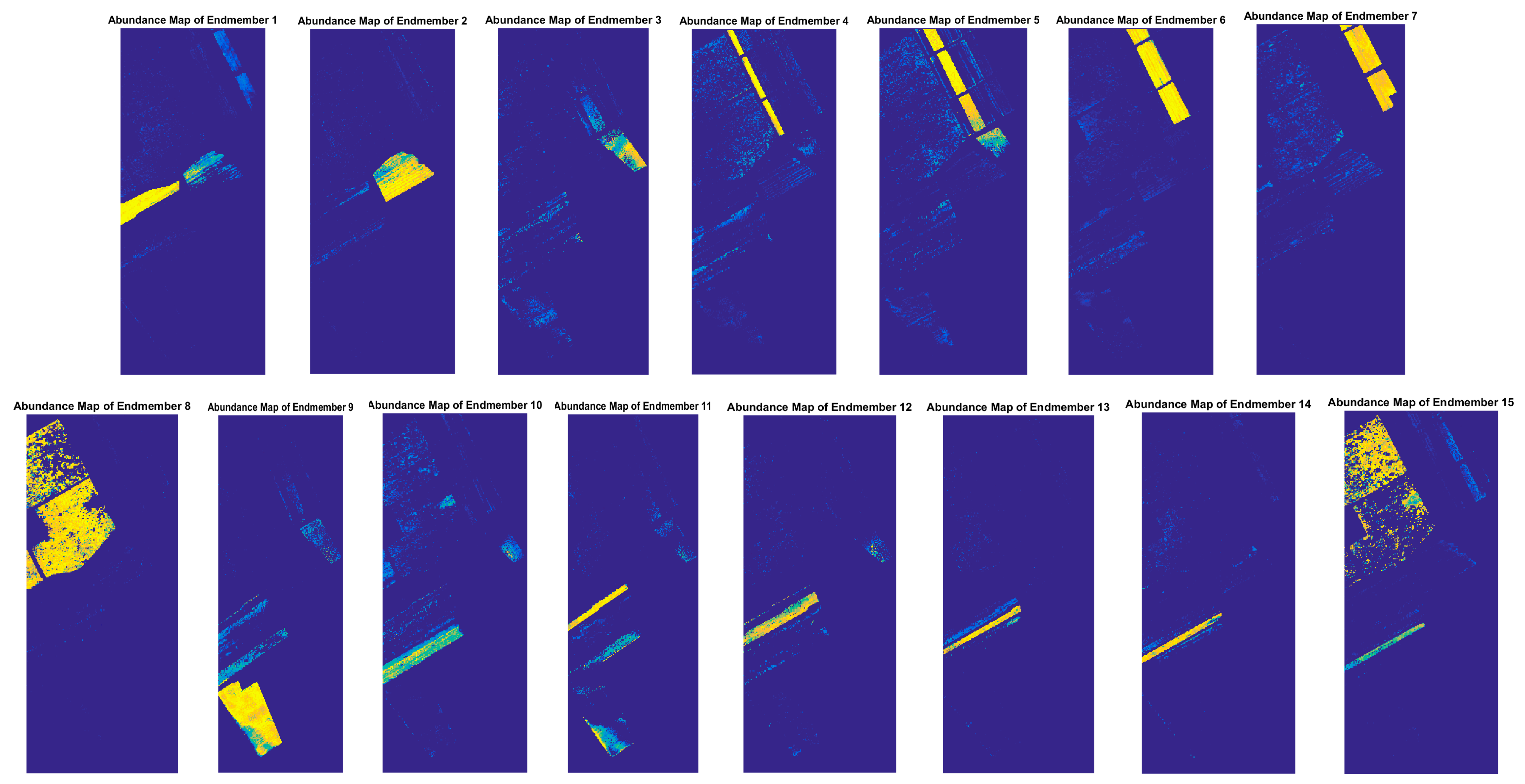
4.3. Experiments on Real Datasets
5. Conclusions
Author Contributions
Conflicts of Interest
References
- Li, C.; Ma, Y.; Mei, X.; Liu, C.; Ma, J. Hyperspectral unmixing with robust collaborative sparse regression. Remote Sens. 2016, 8, 588. [Google Scholar] [CrossRef]
- Liu, R.; Du, B.; Zhang, L. Hyperspectral unmixing via double abundance characteristics constraints based nmf. Remote Sens. 2016, 8, 464. [Google Scholar] [CrossRef]
- Bioucas-Dias, J.M.; Plaza, A.; Dobigeon, N.; Parente, M.; Du, Q.; Gader, P.; Chanussot, J. Hyperspectral unmixing overview: Geometrical, statistical, and sparse regression-based approaches. IEEE J. Sel. Top. Appl. Earth Obs. Remote Sens. 2012, 5, 354–379. [Google Scholar] [CrossRef]
- Somers, B.; Asner, G.P.; Tits, L.; Coppin, P. Endmember variability in spectral mixture analysis: A review. Remote Sens. Environ. 2011, 115, 1603–1616. [Google Scholar] [CrossRef]
- Xu, M.; Zhang, L.; Du, B.; Zhang, L.; Fan, Y.; Song, D. A mutation operator accelerated quantum-behaved particle swarm optimization algorithm for hyperspectral endmember extraction. Remote Sens. 2017, 9, 197. [Google Scholar] [CrossRef]
- Settle, J. On the effect of variable endmember spectra in the linear mixture model. IEEE Trans. Geosci. Remote Sens. 2006, 44, 389–396. [Google Scholar] [CrossRef]
- Iordache, M.D.; Bioucas-Dias, J.M.; Plaza, A. Sparse unmixing of hyperspectral data. IEEE Trans. Geosci. Remote Sens. 2011, 49, 2014–2039. [Google Scholar] [CrossRef]
- Van der Meer, F.D.; Jia, X. Collinearity and orthogonality of endmembers in linear spectral unmixing. Int. J. Appl. Earth Obs. Geoinf. 2012, 18, 491–503. [Google Scholar] [CrossRef]
- Mojaradi, B.; Abrishami-Moghaddam, H.; Zoej, M.J.V.; Duin, R.P.W. Dimensionality reduction of hyperspectral data via spectral feature extraction. IEEE Trans. Geosci. Remote Sens. 2009, 47, 2091–2105. [Google Scholar] [CrossRef]
- Zare, A.; Ho, K. Endmember variability in hyperspectral analysis: Addressing spectral variability during spectral unmixing. IEEE Signal Proc. Mag. 2014, 31, 95–104. [Google Scholar] [CrossRef]
- Xu, X.; Tong, X.; Plaza, A.; Zhong, Y.; Xie, H.; Zhang, L. Joint sparse sub-pixel mapping model with endmember variability for remotely sensed imagery. Remote Sens. 2016, 9, 15. [Google Scholar] [CrossRef]
- Asner, G.P.; Lobell, D.B. A biogeophysical approach for automated swir unmixing of soils and vegetation. Remote Sens. Environ. 2000, 74, 99–112. [Google Scholar] [CrossRef]
- Somers, B.; Delalieux, S.; Verstraeten, W.; Van Aardt, J.; Albrigo, G.; Coppin, P. An automated waveband selection technique for optimized hyperspectral mixture analysis. Int. J. Remote Sens. 2010, 31, 5549–5568. [Google Scholar] [CrossRef]
- Richards, J.A. Remote Sensing Digital Image Analysis: An Introduction; Springer: Berlin, Germany, 2012. [Google Scholar]
- Green, A.A.; Berman, M.; Switzer, P.; Craig, M.D. A transformation for ordering multispectral data in terms of image quality with implications for noise removal. IEEE Trans. Geosci. Remote Sens. 1988, 26, 65–74. [Google Scholar] [CrossRef]
- Wang, L.; Jia, X.; Zhang, Y. A novel geometry-based feature-selection technique for hyperspectral imagery. IEEE Geosci. Remote Sens. Lett. 2007, 4, 171–175. [Google Scholar] [CrossRef]
- Du, Q.; Yang, H. Similarity-based unsupervised band selection for hyperspectral image analysis. IEEE Geosci. Remote Sens. Lett. 2008, 5, 564–568. [Google Scholar] [CrossRef]
- Asl, M.G.; Mobasheri, M.R.; Mojaradi, B. Unsupervised feature selection using geometrical measures in prototype space for hyperspectral imagery. IEEE Trans. Geosci. Remote Sens. 2014, 52, 3774–3787. [Google Scholar]
- Somers, B.; Zortea, M.; Plaza, A.; Asner, G.P. Automated extraction of image-based endmember bundles for improved spectral unmixing. IEEE J. Sel. Top. Appl. Earth Obs. Remote Sens. 2012, 5, 396–408. [Google Scholar] [CrossRef]
- Winter, M.E. N-findr: An Algorithm for Fast Autonomous Spectral End-Member Determination in Hyperspectral Data. In Proceedings of the SPIE’s International Symposium on Optical Science, Engineering, and Instrumentation, Denver, CO, USA, 27 October 1999. [Google Scholar]
- Harsanyi, J.C.; Chang, C.-I. Hyperspectral image classification and dimensionality reduction: An orthogonal subspace projection approach. IEEE Trans. Geosci. Remote Sens. 1994, 32, 779–785. [Google Scholar] [CrossRef]
- Chang, C.I. Hyperspectral Imaging: Techniques for Spectral Detection and Classification; Springer: New York, NY, USA, 2003; Volume 1. [Google Scholar]
- Neville, R.; Staenz, K.; Szeredi, T.; Lefebvre, J.; Hauff, P. Automatic Endmember Extraction from Hyperspectral Data for Mineral Exploration. In Proceedings of the 21st Canadian Symposium on Remote Sens, Ottawa, ON, Canada, 21–24 June 1999. [Google Scholar]
- Nascimento, J.M.P.; Dias, J.M.B. Vertex component analysis: A fast algorithm to unmix hyperspectral data. IEEE Trans. Geosci. Remote Sens. 2005, 43, 898–910. [Google Scholar] [CrossRef]
- Chang, C.-I.; Chen, S.-Y.; Li, H.-C.; Chen, H.-M.; Wen, C.-H. Comparative study and analysis among atgp, vca, and sga for finding endmembers in hyperspectral imagery. IEEE J. Sel. Top. Appl. Earth Obs. Remote Sens. 2016, 9, 4280–4306. [Google Scholar] [CrossRef]
- Chang, C.I.; Wu, C.C.; Liu, W.; Ouyang, Y.C. A new growing method for simplex-based endmember extraction algorithm. IEEE Trans. Geosci. Remote Sens. 2006, 44, 2804–2819. [Google Scholar] [CrossRef]
- Martin, G.; Plaza, A. Spatial-spectral preprocessing prior to endmember identification and unmixing of remotely sensed hyperspectral data. IEEE J. Sel. Top. Appl. Earth Obs. Remote Sens. 2012, 5, 380–395. [Google Scholar] [CrossRef]
- Bioucas-Dias, J.M.; Nascimento, J.M. Hyperspectral subspace identification. IEEE Trans. Geosci. Remote Sens. 2008, 46, 2435–2445. [Google Scholar] [CrossRef]
- Boardman, J.W.; Kruse, F.A.; Green, R.O. Mapping Target Signatures via Partial Unmixing of Aviris dData. In Proceedings of the Fifth Annual JPL Airborne Earth Science Workshop, Pasadena, CA, USA, 23–26 January 1995. [Google Scholar]
- Rodriguez, A.; Laio, A. Clustering by fast search and find of density peaks. Science 2014, 344, 1492–1496. [Google Scholar] [CrossRef] [PubMed]
- Chang, C.-I.; Wang, S. Constrained band selection for hyperspectral imagery. IEEE Trans. Geosci. Remote Sens. 2006, 44, 1575–1585. [Google Scholar] [CrossRef]
- Chang, C.-I.; Du, Q.; Sun, T.-L.; Althouse, M.L. A joint band prioritization and band-decorrelation approach to band selection for hyperspectral image classification. IEEE Trans. Geosci. Remote Sens. 1999, 37, 2631–2641. [Google Scholar] [CrossRef]
- Heinz, D.C.; Chang, C.-I. Fully constrained least squares linear spectral mixture analysis method for material quantification in hyperspectral imagery. IEEE Trans. Geosci. Remote Sens. 2001, 39, 529–545. [Google Scholar] [CrossRef]
- Hyperspectral Imagery Synthesis Tools for Matlab. Available online: http://www.ehu.es/ccwintco/index.php/Hyperspectral_Imagery_Synthesis_tools_for_MATLAB (accessed on 21 March 2017).
- Nascimento, J.M.P. Unsupervised Hyperspectral Unmixing; Universidade Técnica de Lisboa: Lisbon, Portugal, 2006. [Google Scholar]
- Shaw, G.A.; Burke, H.-H.K. Spectral imaging for remote sensing. Linc. Lab. J. 2003, 14, 3–28. [Google Scholar]
- Russell Ranch Sustainable Agriculture Facility. Available online: http://asi.ucdavis.edu/programs/rr (accessed on 10 March 2017).
- Photos and Maps—Agricultural Sustainability Institute—Uc Davis. Available online: http://asi.ucdavis.edu/programs/rr/photos-and-maps (accessed on 15 March 2017).
- Chang, C.-I. An information-theoretic approach to spectral variability, similarity, and discrimination for hyperspectral image analysis. IEEE Trans. Inf. Theory 2000, 46, 1927–1932. [Google Scholar] [CrossRef]


| Dataset 1 | Dataset 2 | Dataset 3 | Dataset 4 | Dataset 5 | |
|---|---|---|---|---|---|
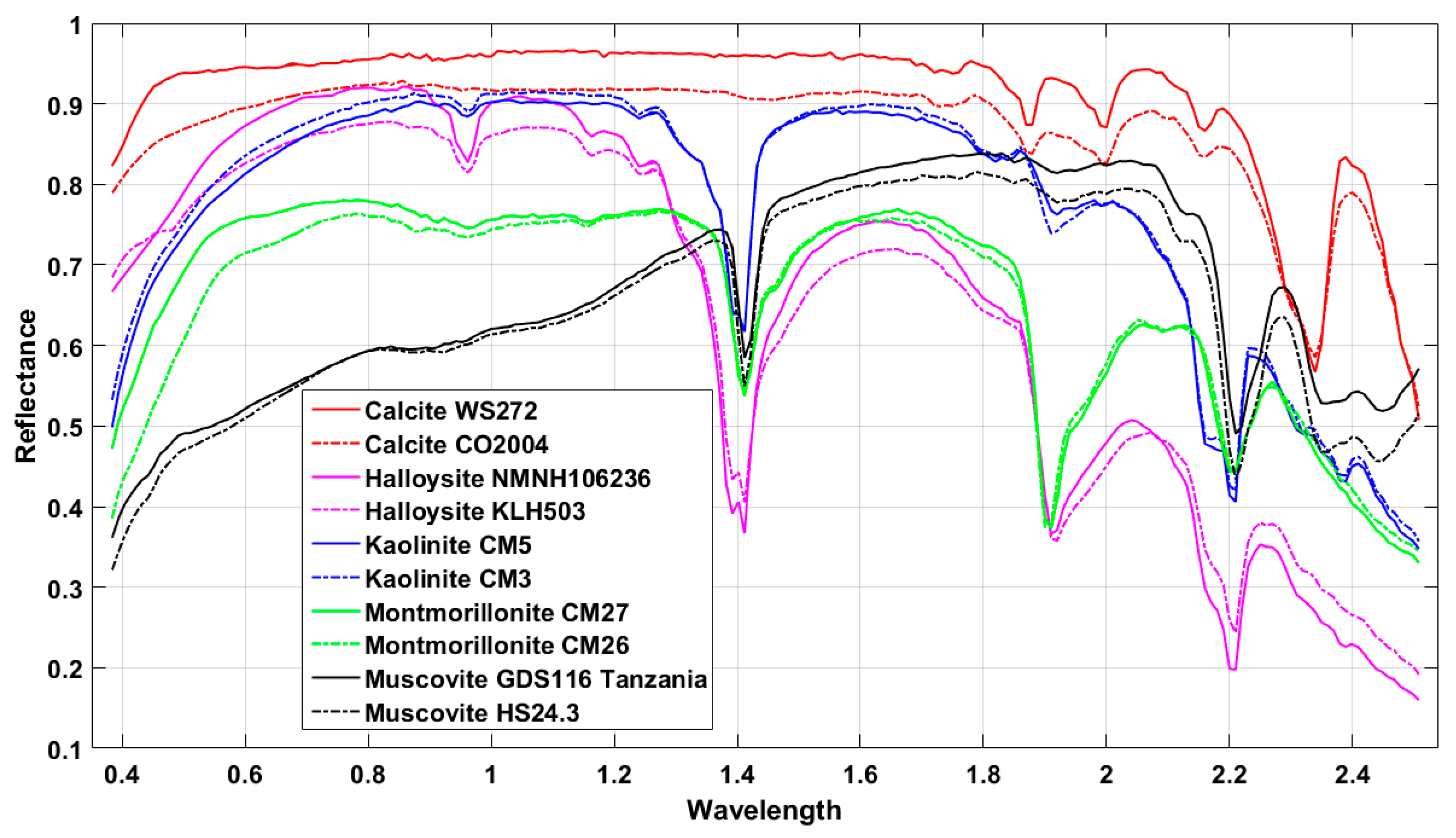
| Mineral | Alunite HS295.3B Calcite HS48.3B Epidote HS328.3B Kaolinite CM3 Montmorillonite CM20 | Alunite HS295.3B Dickite NMNH106242 Halloysite CM13 Kaolinite CM3 Montmorillonite CM20 | Alunite HS295.3B Halloysite NMNH106 Kaolinite KGa-1 (wxyl) Montmorillonite CM20 Muscovite GDS116 | Alunite HS295.3B Calcite HS48.3B Chlorite HS179.3B Epidote HS328.3B Hematite GDS27 Kaolinite CM3 Montmorillonite CM20 | Calcite WS272, CO2004 Halloysite NMNH106, KLH503 Kaolinite CM5, CM3 Montmorillonite CM27, CM26 Muscovite GDS116, HS24.3 |
| Abundance Map Pattern | Spherical Gaussian Fields | Exponential Gaussian Fields | Rational Gaussian Fields | Mattern Gaussian Fields | Mattern Gaussian Fields |
| Data Set | Feature Selection Method | Full Dimensionality | |||||||||||||||||
|---|---|---|---|---|---|---|---|---|---|---|---|---|---|---|---|---|---|---|---|
| ISI-PS | SZU | MTD | |||||||||||||||||
| Abundance Map | #S | SNR | #F | Cond | Corr | RMSE | #F | Cond | Corr | RMSE | #F | T | Cond | Corr | RMSE | #F | Cond | Corr | RMSE |
| Spherical | 5 | 20:1 | 63 | 21.01 | 0.39 | 0.071 | 55 | 28.87 | 0.42 | 0.083 | 29 | 4.00 | 20.97 | 0.40 | 0.071 | 224 | 30.40 | 0.41 | 0.085 |
| Exponential | 5 | 25:1 | 43 | 30.09 | 0.70 | 0.105 | 24 | 117.39 | 0.90 | 0.153 | 27 | 4.00 | 28.99 | 0.68 | 0.103 | 224 | 48.72 | 0.87 | 0.148 |
| Rational | 5 | 30:1 | 68 | 40.98 | 0.51 | 0.090 | 67 | 55.82 | 0.58 | 0.101 | 34 | 3.25 | 36.88 | 0.55 | 0.083 | 224 | 70.58 | 0.53 | 0.112 |
| Mattern | 7 | 25:1 | 61 | 39.54 | 0.19 | 0.063 | 54 | 58.88 | 0.27 | 0.070 | 38 | 3.75 | 38.04 | 0.22 | 0.061 | 224 | 52.50 | 0.21 | 0.068 |
| Mattern | 10 | 30:1 | 65 | 49.71 | 0.58 | 0.181 | 67 | 61.08 | 0.64 | 0.183 | 14 | 4.75 | 34.84 | 0.57 | 0.180 | 224 | 81.72 | 0.61 | 0.187 |
| Data Set | Feature Selection Method | Full Dimensionality | |||||||||||||||||
|---|---|---|---|---|---|---|---|---|---|---|---|---|---|---|---|---|---|---|---|
| ISI-PS | SZU | MTD | |||||||||||||||||
| Abundance Map | #S | SNR | #F | Cond | Corr | RMSE | #F | Cond | Corr | RMSE | #F | T | Cond | Corr | RMSE | #F | Cond | Corr | RMSE |
| Spherical | 5 | 20:1 | 61 | 20.77 | 0.41 | 0.047 | 138 | 25.81 | 0.42 | 0.050 | 30 | 4.00 | 19.95 | 0.44 | 0.047 | 224 | 32.41 | 0.44 | 0.053 |
| Exponential | 5 | 25:1 | 42 | 28.09 | 0.67 | 0.057 | 124 | 38.88 | 0.82 | 0.062 | 24 | 4.25 | 28.12 | 0.65 | 0.055 | 224 | 45.31 | 0.86 | 0.067 |
| Rational | 5 | 30:1 | 70 | 44.58 | 0.61 | 0.071 | 109 | 62.38 | 0.58 | 0.074 | 23 | 4.00 | 36.43 | 0.60 | 0.068 | 224 | 76.40 | 0.62 | 0.075 |
| Mattern | 7 | 25:1 | 61 | 36.41 | 0.19 | 0.043 | 109 | 45.14 | 0.25 | 0.044 | 40 | 3.75 | 33.31 | 0.23 | 0.043 | 224 | 46.38 | 0.21 | 0.044 |
| Mattern | 10 | 30:1 | 55 | 43.32 | 0.55 | 0.175 | 152 | 70.40 | 0.59 | 0.175 | 12 | 3.00 | 34.58 | 0.53 | 0.174 | 224 | 74.47 | 0.60 | 0.176 |
| Data Set | Feature Selection Method | Full Dimensionality | ||||||||||||
|---|---|---|---|---|---|---|---|---|---|---|---|---|---|---|
| MTD | SZU | ISI-PS | ||||||||||||
| Name | #S | #F | Cond Corr | Abun RMSE | #F | Cond Corr | Abun RMSE | #F | Cond Corr | Abun RMSE | T | #F | Cond Corr | Abun RMSE |
| IMG RMSE | IMG RMSE | IMG RMSE | IMG RMSE | |||||||||||
| LTRAS | 7 | 31 | 221.41 | 0.753 | 83 | 214.41 | 0.797 | 46 | 203.10 | 0.686 | 1.25 | 170 | 230.08 | 0.873 |
| (supervised) | 0.73 | 0.1730 | 0.74 | 0.1343 | 0.68 | 0.1570 | 0.69 | 0.1619 | ||||||
| LTRAS | 9 | 20 | 327.48 | 0.573 | 81 | 385.38 | 0.556 | 61 | 421.11 | 0.500 | 0.85 | 170 | 400.32 | 0.631 |
| (unsupervised) | 0.76 | 0.1360 | 0.72 | 0.1435 | 0.67 | 0.1309 | 0.71 | 0.1393 | ||||||
| Salinas | 15 | 31 | 12,996.30 | 0.860 | 45 | 15,150.40 | 0.845 | 43 | 12,911.04 | 0.843 | 0.55 | 160 | 11,332.69 | 0.856 |
| (supervised) | 0.89 | 0.0410 | 0.86 | 0.0395 | 0.84 | 0.0398 | 0.88 | 0.0382 | ||||||
| Salinas | 15 | 29 | 9480.33 | 0.421 | 52 | 7554.07 | 0.416 | 49 | 6444.09 | 0.395 | 0.40 | 160 | 5896.17 | 0.398 |
| (unsupervised) | 0.87 | 0.0343 | 0.84 | 0.0327 | 0.80 | 0.0315 | 0.87 | 0.0290 | ||||||
| Indiana | 12 | 29 | 10,563.01 | 2.245 | 30 | 11,765.44 | 2.130 | 38 | 9858.71 | 2.086 | 0.35 | 166 | 6723.01 | 2.219 |
| (supervised) | 0.94 | 0.1647 | 0.95 | 0.1680 | 0.92 | 0.1655 | 0.94 | 0.1456 | ||||||
| Indiana | 11 | 20 | 2533.14 | 1.349 | 29 | 3237.09 | 1.262 | 28 | 1459.26 | 1.240 | 0.50 | 166 | 1656.70 | 1.261 |
| (unsupervised) | 0.92 | 0.1091 | 0.92 | 0.1008 | 0.90 | 0.0970 | 0.93 | 0.0977 | ||||||
| SID | Extracted Endmembers | |||||||||
|---|---|---|---|---|---|---|---|---|---|---|
| 1 | 2 | 3 | 4 | 5 | 6 | 7 | 8 | 9 | ||
| Reference Endmembers | Corn | 0.0059 | 0.3061 | 0.7046 | 0.4647 | 0.5015 | 0.0193 | 0.0276 | 0.0036 | 0.0364 |
| Alfalfa | 0.1727 | 0.0000 | 0.0879 | 0.0303 | 0.0248 | 0.2226 | 0.1535 | 0.3621 | 0.5499 | |
| Fallow | 0.4828 | 0.0841 | 0.0001 | 0.0400 | 0.0223 | 0.5478 | 0.4532 | 0.7745 | 1.0368 | |
| Wheat | 0.3406 | 0.0421 | 0.0231 | 0.0031 | 0.0112 | 0.3921 | 0.3287 | 0.6076 | 0.8386 | |
| Native Grass | 0.3090 | 0.0215 | 0.0271 | 0.0126 | 0.0003 | 0.3709 | 0.2861 | 0.5548 | 0.7830 | |
| Tomato | 0.0062 | 0.1768 | 0.4826 | 0.2778 | 0.3245 | 0.0028 | 0.0155 | 0.0538 | 0.1236 | |
| W.S. | 0.0240 | 0.1667 | 0.4879 | 0.2987 | 0.3176 | 0.0199 | 0.0003 | 0.0383 | 0.1133 | |
| Dataset | CPU Time (s) | |||
|---|---|---|---|---|
| Feature Selection Methods | Full Bands | |||
| MTD | SZU | ISI-PS | ||
| LTRAS | 10.94 | 11.34 | 78.72 | 10.92 |
| Salinas | 107.43 | 107.71 | 620.90 | 117.73 |
| Indiana Pines | 14.93 | 14.92 | 91.13 | 15.66 |
© 2017 by the authors. Licensee MDPI, Basel, Switzerland. This article is an open access article distributed under the terms and conditions of the Creative Commons Attribution (CC BY) license (http://creativecommons.org/licenses/by/4.0/).
Share and Cite
Ghaffari, O.; Zoej, M.J.V.; Mokhtarzade, M. Reducing the Effect of the Endmembers’ Spectral Variability by Selecting the Optimal Spectral Bands. Remote Sens. 2017, 9, 884. https://doi.org/10.3390/rs9090884
Ghaffari O, Zoej MJV, Mokhtarzade M. Reducing the Effect of the Endmembers’ Spectral Variability by Selecting the Optimal Spectral Bands. Remote Sensing. 2017; 9(9):884. https://doi.org/10.3390/rs9090884
Chicago/Turabian StyleGhaffari, Omid, Mohammad Javad Valadan Zoej, and Mehdi Mokhtarzade. 2017. "Reducing the Effect of the Endmembers’ Spectral Variability by Selecting the Optimal Spectral Bands" Remote Sensing 9, no. 9: 884. https://doi.org/10.3390/rs9090884
APA StyleGhaffari, O., Zoej, M. J. V., & Mokhtarzade, M. (2017). Reducing the Effect of the Endmembers’ Spectral Variability by Selecting the Optimal Spectral Bands. Remote Sensing, 9(9), 884. https://doi.org/10.3390/rs9090884