Article

Characteristics of Evapotranspiration of Urban Lawns in a Sub-Tropical Megacity and Its Measurement by the ‘Three Temperature Model + Infrared Remote Sensing’ Method

Shenzhen Engineering Laboratory for Water Desalination with Renewable Energy, School of Environment and Energy, Peking University, Beijing 100871, China
*
Authors to whom correspondence should be addressed.
Remote Sens. 2017, 9(5), 502; https://doi.org/10.3390/rs9050502
Submission received: 13 March 2017 / Revised: 3 May 2017 / Accepted: 14 May 2017 / Published: 19 May 2017

Abstract

:
Evapotranspiration (ET) is one of the most important factors in urban water and energy regimes. Because of the extremely high spatial heterogeneity of urban area, accurately measuring ET using conventional methods remains a challenge due to their fetch requirements and low spatial resolution. The goals of this study were to investigate the characteristics of urban ET and its main influencing factors and subsequently to improve a fetch-free, high spatial resolution method for urban ET estimation. The Bowen ratio and the ‘three-temperature model (3T model) + infrared remote sensing (RS)’ methods were used for these purposes. The results of this study are listed in the following lines. (1) Urban ET is mainly affected by solar radiation and the effects of air humidity, wind velocity, and air temperature are very weak; (2) The average daily, monthly, and annual ETs of the urban lawn are 2.70, 60–100, and 990 mm, respectively, which are obvious compared with other landscapes; (3) The ratio of ET to precipitation is 0.65 in the wet season and 2.6 in the dry season, indicating that most of the precipitation is evaporated; (4) The fetch-free approach of ‘3T model + infrared RS’ is verified to be an accurate method for measuring urban ET and it agrees well with the Bowen ratio method (R2 is over 0.93 and the root mean square error is less than 0.04 mm h−1); (5) The spatial heterogeneity of urban ET can also be accurately estimated by the proposed approach. These results are helpful for improving the accuracy of ET estimation in urban areas and are useful for urban water and environmental planning and management.

Graphical Abstract

1. Introduction

There are usually two strategies to mitigate the urban heat island. One is to increase the surface reflectance (albedo) of urban surface materials (building and pavement), which can reflect more short wave solar irradiance back to the space and reduce the net energy income of urban area [1]. This can be achieved by using high reflectance building material, or coating and painting technologies [2]. Another strategy is to increase evapotranspiration (ET) of urban area, which can use the absorbed solar energy by latent heat and then decrease air temperature [3]. Actually, ET is one of the most important components of the water budget and energy balance in urban environments. It has been extensively researched and applied to water and environmental quality management in agricultural and natural ecosystems. However, few researchers focus on urban ET, and it may be the least-studied part of urban hydrology [4,5,6,7]. According to Grimmond and Oke [4], urban ET is usually regarded far lower than that in rural areas because ground of urban area is covered by buildings and paved roads. Therefore, ET in urban areas has been considered negligible in many cases [4]. Moreover, the urban surface is composed of complex underlying covers, including buildings, roads, vegetation, and water bodies. The large spatial heterogeneity makes it extremely difficult to measure urban ET using many of the conventional methods.
The rapid development of global urbanization, however, is creating a series of ecological and environmental problems for the people living in urban areas [8], such as increased risks of urban heat islands and floods, water shortages, and water pollution. Most of these challenges are closely related to the urban ET. In urban environments, large areas of permeable and moist soil are replaced by artificial impermeable surfaces (cement, asphalt, etc.), which greatly change the physical properties of the land surface. This trend is further worsened by human activities introduced changes to the water and energy cycles. These changes increase the intensity of urban heat islands [9,10], urban rain islands, and waterlogging [11,12,13]. Urban ET, as the only factor connecting the energy balance and water budget in urban areas, is an unavoidable factor in urban water management and living environment maintenance.
In fact, a few recent studies have showed that urban ET is quite large and is an important part of urban water budget [5,9,14,15,16]. It is widely recognized that urban ET can relieve the heat island effect and reduce storm floods [17,18,19]. Experimental and simulation studies on green roofs show that ET can significantly reduce urban temperature [20,21]. In addition, as a source of water vapor, urban ET is very important for the urban climate [5]. Actually, some pioneer cities have put ET into their environmental management evaluation framework. According to the reports of Philadelphia and New York City, urban green projects can possibly provide an added value to the urban environment, which may have worth of hundreds of millions to billions of dollars [22,23]. Therefore, the accurate determination of urban ET is essential for urban hydrology, water management, and ecological and environmental planning and management [24,25,26].
Despite its importance, up to now only few studies have focused on urban ET. Grimmond and Oke [4] measured urban ET using the eddy covariance method and found that ET could reach approximately 1–3 mm day−1. The related studies began to increase gradually after 2010. Various technologies—such as the sap flow, Bowen ratio, lysimeter, eddy covariance, and large aperture scintillometer—have gradually been used in urban ET measurement. Pataki et al. [27] measured the transpiration rate of 15 species of trees using the sap flow method in Los Angeles. They found that ficus, United States shittim, and California sycamores had higher transpiration rates, whereas American redwood had lower transpiration rates. Peters et al. [28] studied the seasonal change of urban ET using the sap flow, Bowen ratio, and eddy covariance methods. Their results showed that turf grasses used more water than trees in Minneapolis-Saint Paul area. DiGiovanni et al. [19] measured ET at six locations in New York City using lysimeter and found that there were significant differences in ET among different green land types. Jacobs et al. [29] measured the urban ET using the eddy covariance, sap flow, and large aperture scintillometers in Arnhem and Rotterdam in the Netherlands. The results showed that ET was 0.5–1.0 mm day−1 in the two cities, whereas the transpiration rate of the trees was on average 170 liters per day, which contributed considerably to the local ET. Jacobs also noted that there is no linear relationship between the urban reference ET and actual ET due to the complexity of the city ground surface [29]. Ward et al. [30] observed urban ET using a large aperture scintillometer in Swindon of Britain. In his study, the measured ET was 1–3 mm day−1 on average, which was greater than the eddy covariance measured urban ET (0.5–2.0 mm day−1). At the 2015 AGU fall conference, more studies reported their results on urban ET, including ET estimation methods, time and space variations, and driving factors [3,31,32,33,34].
Based on these carefully designed pioneer studies, it is clear that urban ET is a very important component of the urban water and energy cycles. It is also revealed that, although these conventional methods are mature, it is still a challenge to obtain accurate ET by using these methods in urban [5,35]. This is because it is very difficult to meet their fetch requirements and their low spatial resolution. A fetch-free and high spatial resolution ET estimation method is highly needed for urban water and environmental management.
Hence, the goals of this study are to investigate the characteristics of urban ET and its main affecting factor and then to improve a fetch-free, high spatial resolution method for urban ET estimation.

2. Materials and Methods

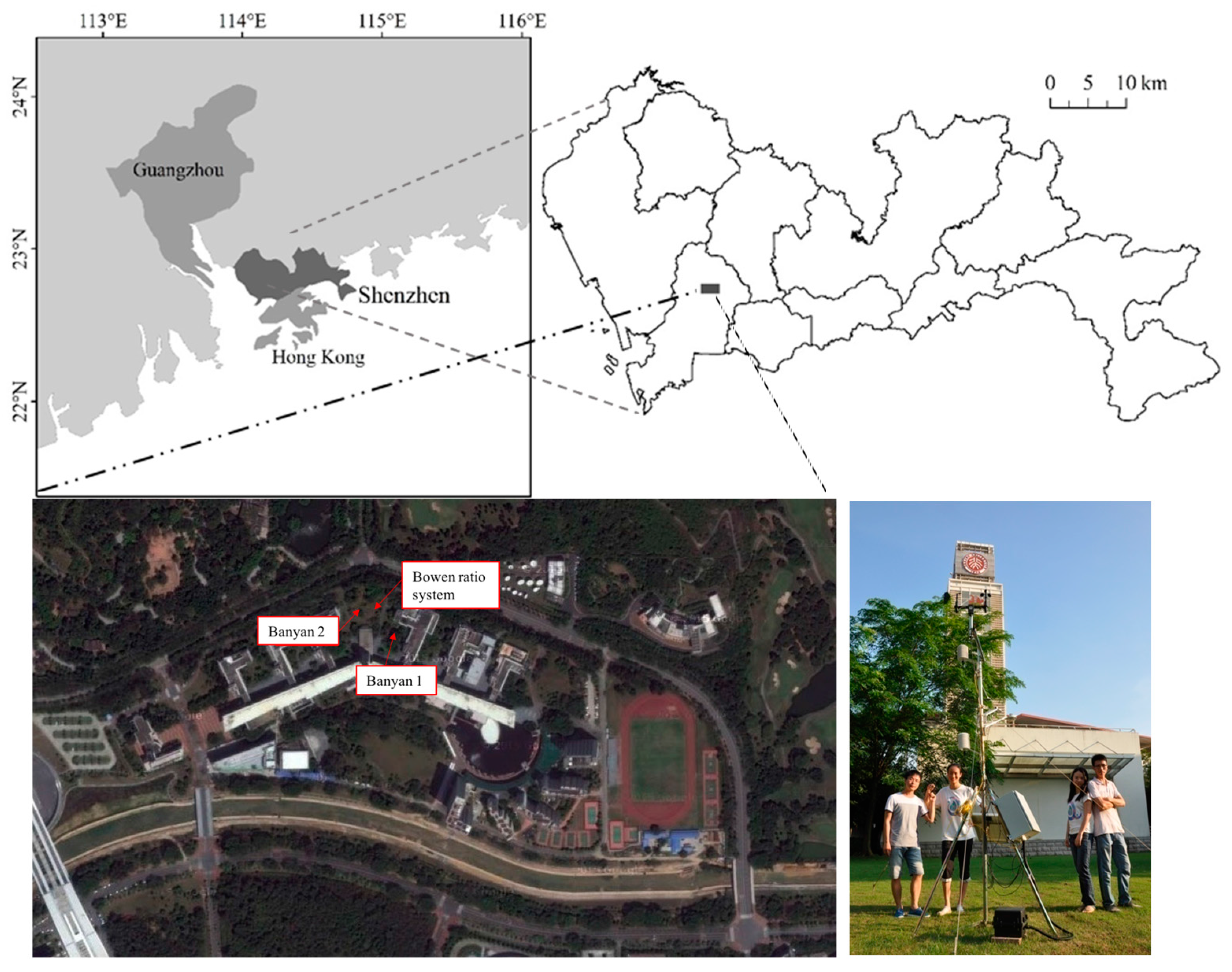
2.1. Study Site and Measurements

The study area was located in Xili University Town (about 22°35′40″N, 113°58′20″E, 17 m above sea level), Shenzhen (Figure 1), which is a part of the most densely populated sub-tropical megacity in China. The study area was covered by different vegetation (about 50%) and buildings. Vegetation included tree, bush, and lawn. The height of building was around 20–30 m. Measurement was carried out in a flat lawn field with a size of 300 m in diameter. The plant species of the lawn was Zoysia matrella (L.) Merr., a widely-used lawn species in urban areas in south China. There were a few trees near the observation field and their shadow affected area were excluded when we analyzed the image of surface temperature. A Bowen ratio system tower was established at the central part of this field (photo at the bottom right side in Figure 1).
The experiment was carried out from July 2014 to the end of 2015. The Bowen ratio system was used to measure the meteorological data, including solar radiation, photosynthetic active radiation (PAR), net radiation, the soil heat flux (5 cm under the ground surface, two duplicate samples), the air temperature and humidity at heights of 2 m and 1.5 m. Information regarding the sensor types, measuring height, and sensing resolutions were shown in Table 1. All the data were sampled and recorded at intervals of 1 min and 10 min, respectively, using the Campbell CR1000 data logger.
An infrared thermal camera (IR Flexcam Ti55, Fluke Corp., Everett, WA, USA) was used to measure the surface temperature. The measuring wavelength of the infrared thermal imager was 8–14 µm, and the resolution was 0.05 °C. Each thermal infrared image contains 76,800 temperature data (320 × 240). Measurements were carried from the top of a 50 m-tall tower, which was almost vertically above the canopy. The measurement was carried out every hour in triplicate from 8:00 to 17:00 on sunny, cloudless days. Before the measurement, the thermal camera was calibrated by against a thermocouple-blackbody measurement. Two procedures were taken to avoid the affection of external radiation and other possible uncertainties. First, all the measurements of surface temperature were carried out at the same location and same direction. Secondly, in addition to the measurement from tower, surface temperature was also measured at 2 m above the lawn canopy from different directions, which was used to verify with the data from tower measurement.

2.2. Data Analysis

2.2.1. Estimation of ET by Bowen Ratio Energy Balance (BREB) Method

ET can be expressed as follows by using BREB (Bowen, et al. [36])
ET = R n G L ( 1 + β )
β = C p Δ T L Δ q
where Rn is net radiation (W m−2), L is the latent heat of water vaporization (J kg−1), H is the sensible heat flux (W m−2), G is the soil heat flux (W m−2), β is the Bowen ratio, Cp is the specific heat of air at a constant pressure (J kg−1 °C−1), and ∆T and ∆q are the temperature and humidity difference between the heights of 2.0 m and 1.5 m, respectively.
As required by using the BREB, unqualified data were filtrated out according to the following rules: (1) before sunrise and after sunset and (2) the Bowen ratio was very close to −1. In this study, the data in the range of −0.6 to −1.3 were filtrated out [37,38]. Under this filter rule, data in some periods might be missing. If the amount of missing data was more than 50% of the daily total, daily ET was obtained by averaging the remaining valid instantaneous and then multiplying by the sunshine hours. If the missing data were less than or equal to 50%, adjacent valid data interpolation would be used to fill in the blanks.

2.2.2. Estimation of ET by Using Three Temperature Model (3T Model) + Infrared Remote Sensing (Infrared RS) Method

In the 3T model, by assuming there is a reference leaf (a leaf without transpiration) in the vegetation canopy, ET of fully covered vegetation can be estimated [39,40].
ET = R n R n p T c T a T p T a
where Rnp is the net radiation of the reference leaf (W m−2), Tc is the vegetation surface temperature (K), Tp is the surface temperature of the reference leaf, and Ta is the air temperature (K). In this study, thermal images are taken from the top of the tower every hour in triplicate. From these images, we can get Tc, while the corresponding maximum Tc in the same image is regarded as Tp. Rnp is estimated by using the Tp and solar radiation. All these procedures have been written into a software named ‘A system to estimate evapotranspiration by infrared remote sensing and the three-temperature model’, which can be download and used freely from http://see.pkusz.edu.cn/index.php?m=content&c=index&a=show&catid=1653&id=14.

3. Results

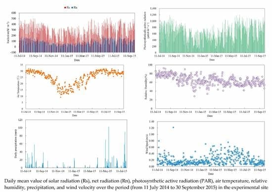
3.1. Meteorological Characteristics in the Studied Urban Area

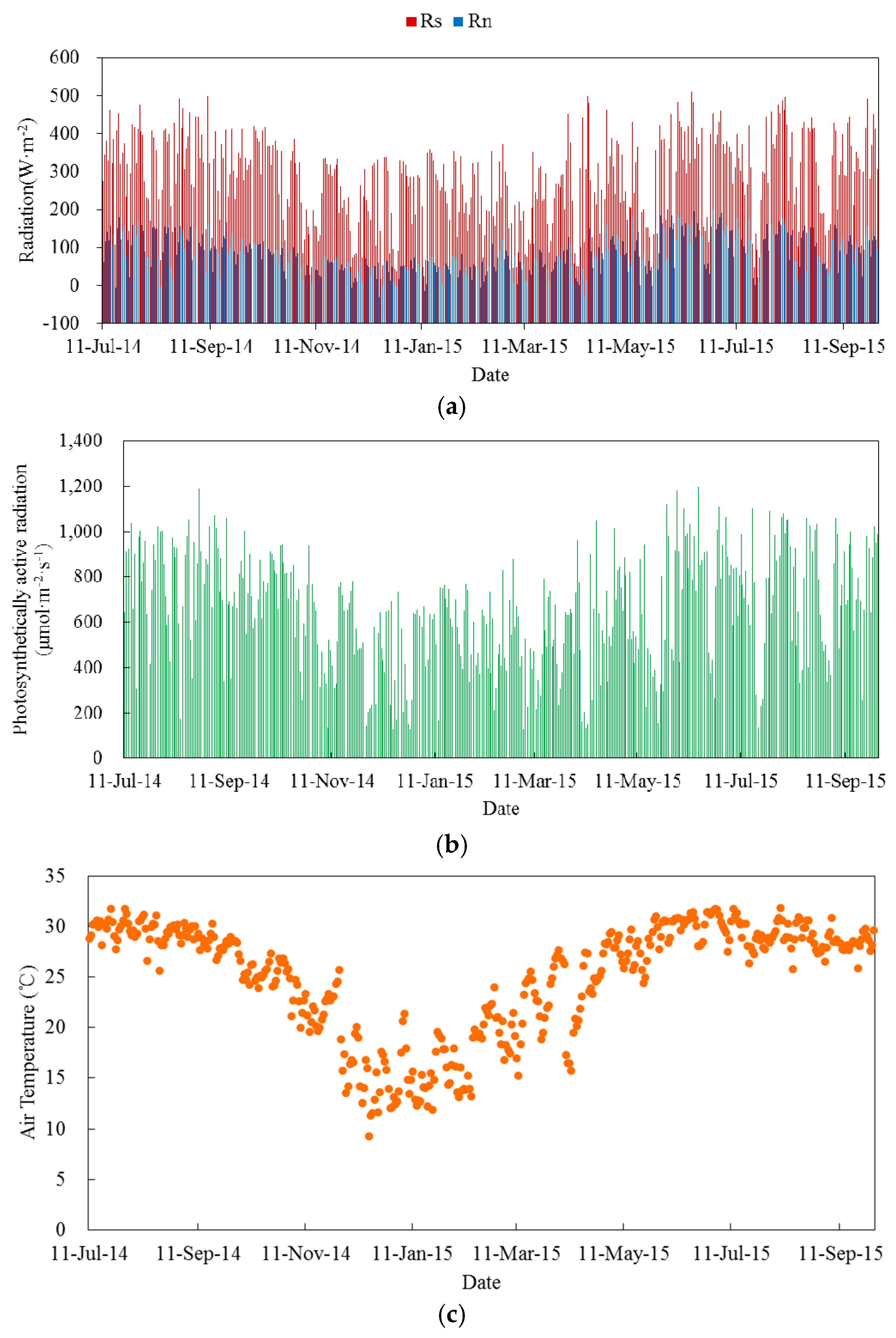
3.1.1. Radiation Characteristics

Radiation is the only energy sources of ET. In this study, we measured solar radiation (Rs), net radiation (Rn), and PAR continuously over the experimental period. To show them more clearly, these values were averaged into daily mean and their variations were shown in Figure 2. It was shown that there were obvious seasonal variations. Rs was high and approximately 300 ± 50 W m−2 in summer and autumn (Table 2), whereas it was low in spring and winter (approximately 200 ± 50 W m−2). The maximum daily average Rs was 520.21 W m−2 (on 28 June 2015) and the minimum was 23.48 W m−2 (on 12 January 2015). From 1 August 2014 to 31 July 2015, the average Rs was 269.61 W m−2. In general, there was plenty of solar radiation in the study area due to its lower latitude.
The daily maximum Rn was 199.04 W m−2 (on 27 July 2015), whereas the minimum value of Rn was −32.50 W m−2 (on 17 December 2014). From 1 August 2014 to 31 July 2015, the daily average Rn was 78.34 W m−2. The average monthly Rn varied from 30.16 to 134.23 W m−2. The maximum appeared in June, and the minimum appeared in December. Rn was significantly higher in the summer period (June, July, and August) than in the other seasons.
PAR showed a similar trend as Rs, being higher in summer and autumn, lower in spring and summer. The daily maximum PAR was 1197.66 μmol m−2 s−1 (on 16 June 2015), and the minimum value was 125.76 μmol m−2 s−1 (on 27 December 2014). The average monthly PAR was in the range of 410.66 to 825.46 μmol m−2 s−1. The annual daily average PAR was 629.16 μmol m−2 s−1 from 1 August 2014 to 31 July 2015.

3.1.2. Air Temperature

The study area had a hot summer and overall high temperatures throughout the year, with obvious seasonal variation (Figure 2). The lowest monthly average temperature was 15.02 °C, recorded in December 2014. August was commonly the monthly temperature peak (Table 2). The average daily temperatures in August 2014 and August 2015 were 29.54 °C and 29.24 °C, respectively. The mean daily temperature was 23.94 °C over the year. The highest daily average temperature was 31.78 °C (on 30 July 2014), and the lowest was 7.05 °C (on 17 December 2014). The temperature difference between day and night time was generally not more than 10 °C, with the highest being 17.09 °C (on 31 December 2014).

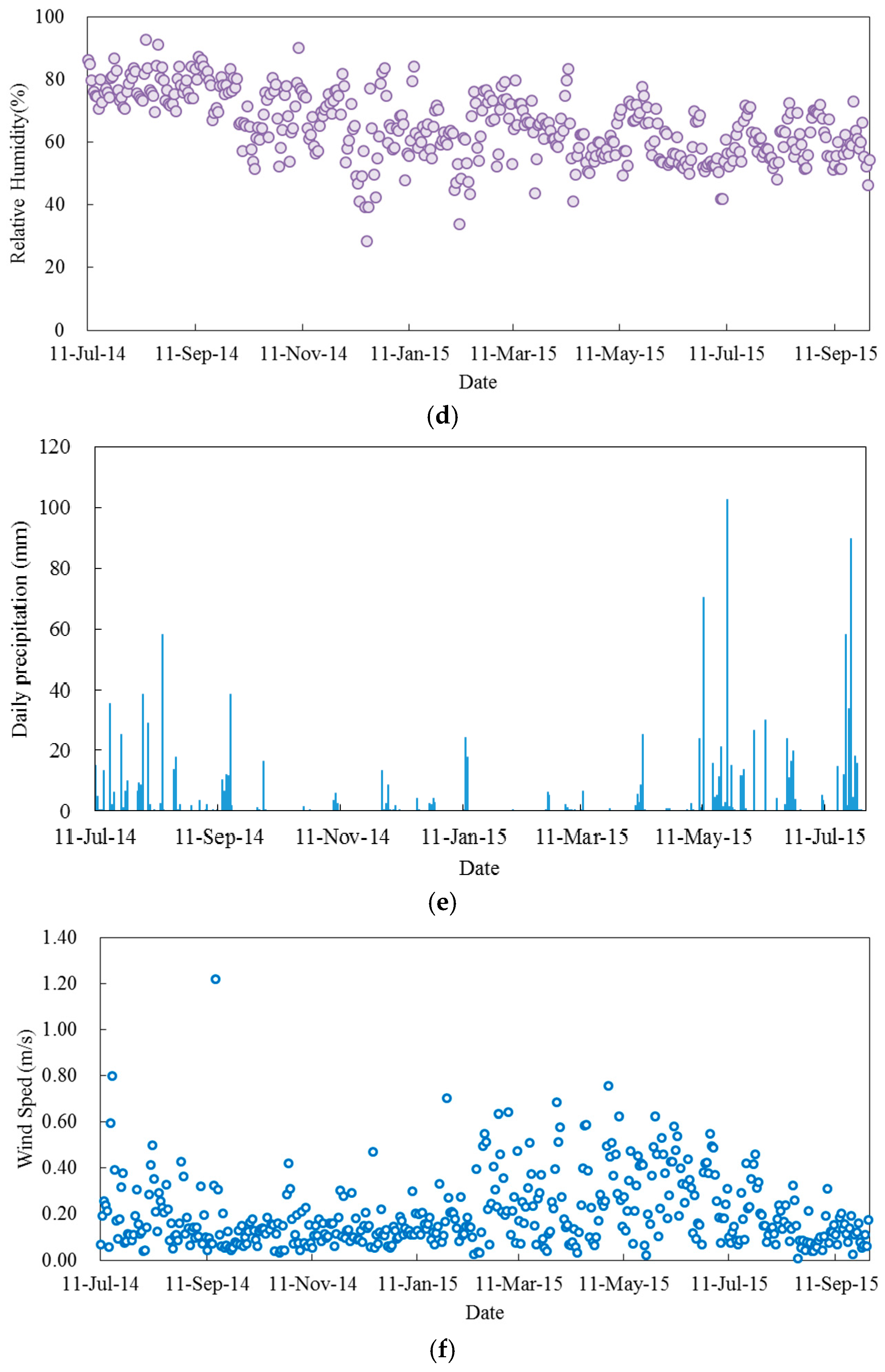
3.1.3. Relative Humidity

From 1 August 2014 to 31 July 2015, the annual mean relative humidity was 65.48%. The lower daily average relative humidity was usually over 40% and most of them were over 60% in the study area (Figure 2). Compared to spring and winter, humidity in summer and autumn was higher (Table 2). The highest daily average was 92.74% (on 13 August 2014) and the minimum was 22.80% (on 17 December 2014). Generally, the study area had high humidity and low vapor pressure deficit (VPD), contributing to the low vapor diffusion speed which could reduce vapor pressure difference between two sensors, which formed the Bowen ratio and lead to the decrease of the ET rate.

3.1.4. Precipitation

The total annual precipitation was 1173.30 mm from 1 August 2014 to 31 July 2015. In the dry season (from October to the following March), rainfall was only 140.20 mm and the remaining 1033.10 mm of precipitation fell in the wet season (from April to September), accounting for 88.05% of the total rainfall of the year. Among them, May to August had more rainfall (monthly over 130 mm). The maximum monthly rainfall was 307.70 mm in May 2015, and the minimum monthly rainfall was only 11.50 mm in March 2015. The daily maximum rainfall was 102.70 mm on 23 May 2015. Generally, the rainfall was in the form of storms (over 30 mm in 12 h). Taking the storm on 23 May 2015 as an example, 68.60 mm of the rainfall fell down in 1 h (15:00–16:00).

3.1.5. Wind Velocity

The wind velocity was generally low and the daily average wind velocity was only 0.21 m s−1 (Figure 2). This was because of the buildings in the urban area. During the year, spring had the highest wind velocity, which was significantly higher than that in the other seasons. The wind velocity in summer was slightly higher than that in autumn and winter.

3.1.6. Summary for Section 3.1

The above results show that the study area is a typical urban area characterized by plenty of solar radiation and precipitation, high humidity, and a lower wind velocity. Because wind velocity has highly spatially sensitive parameters, it is worth investigating its ET characteristics under these specific conditions.

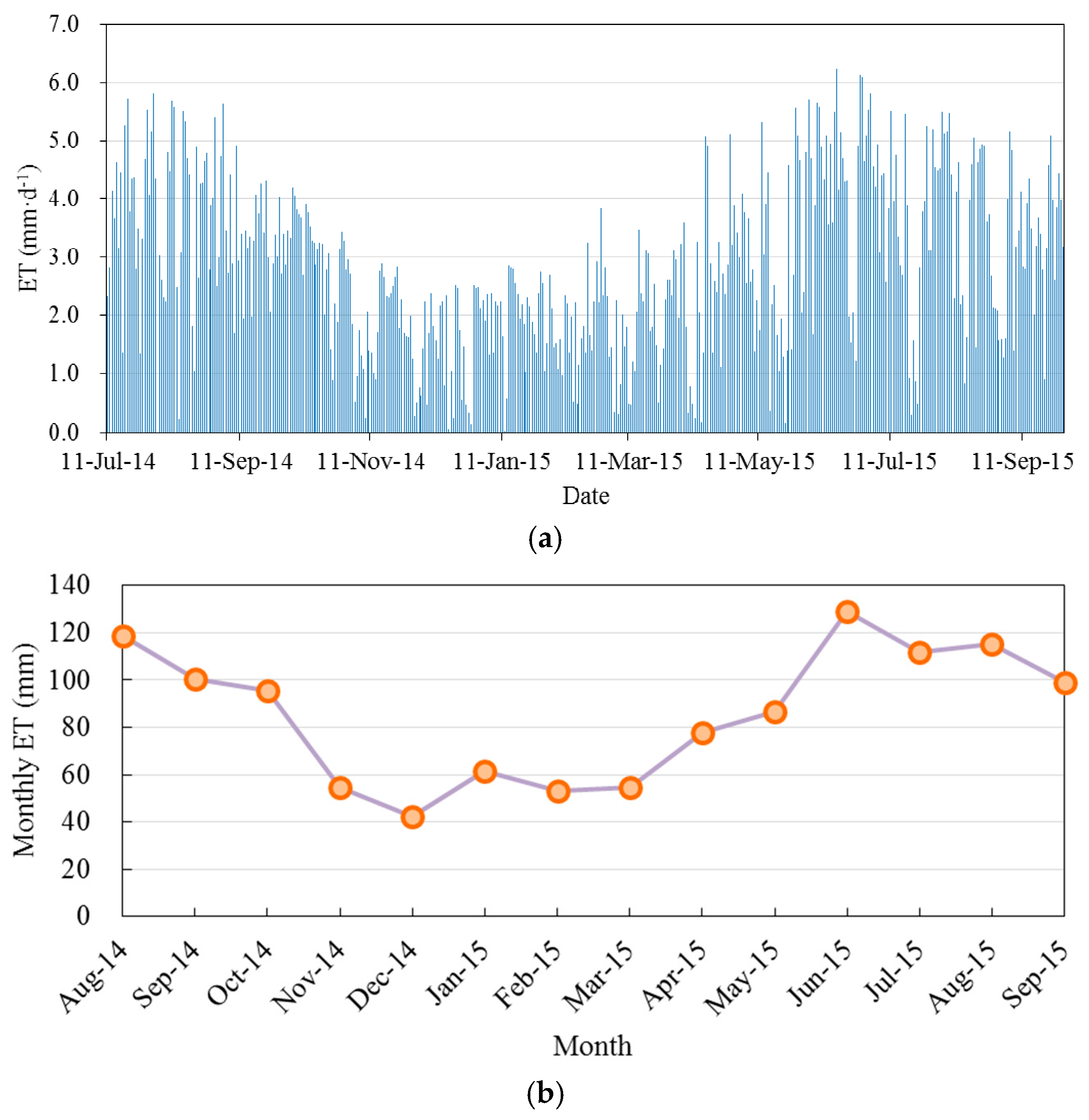
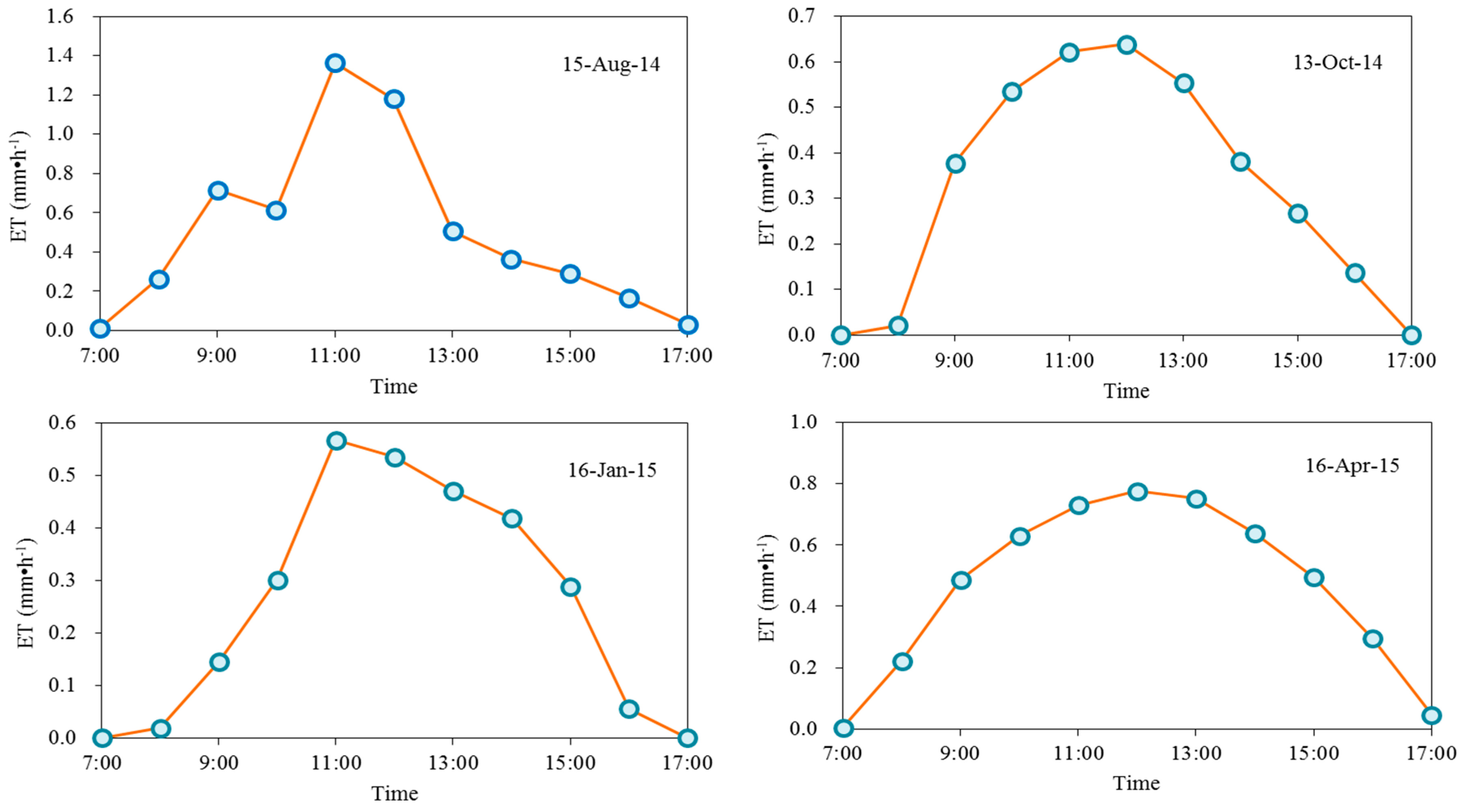
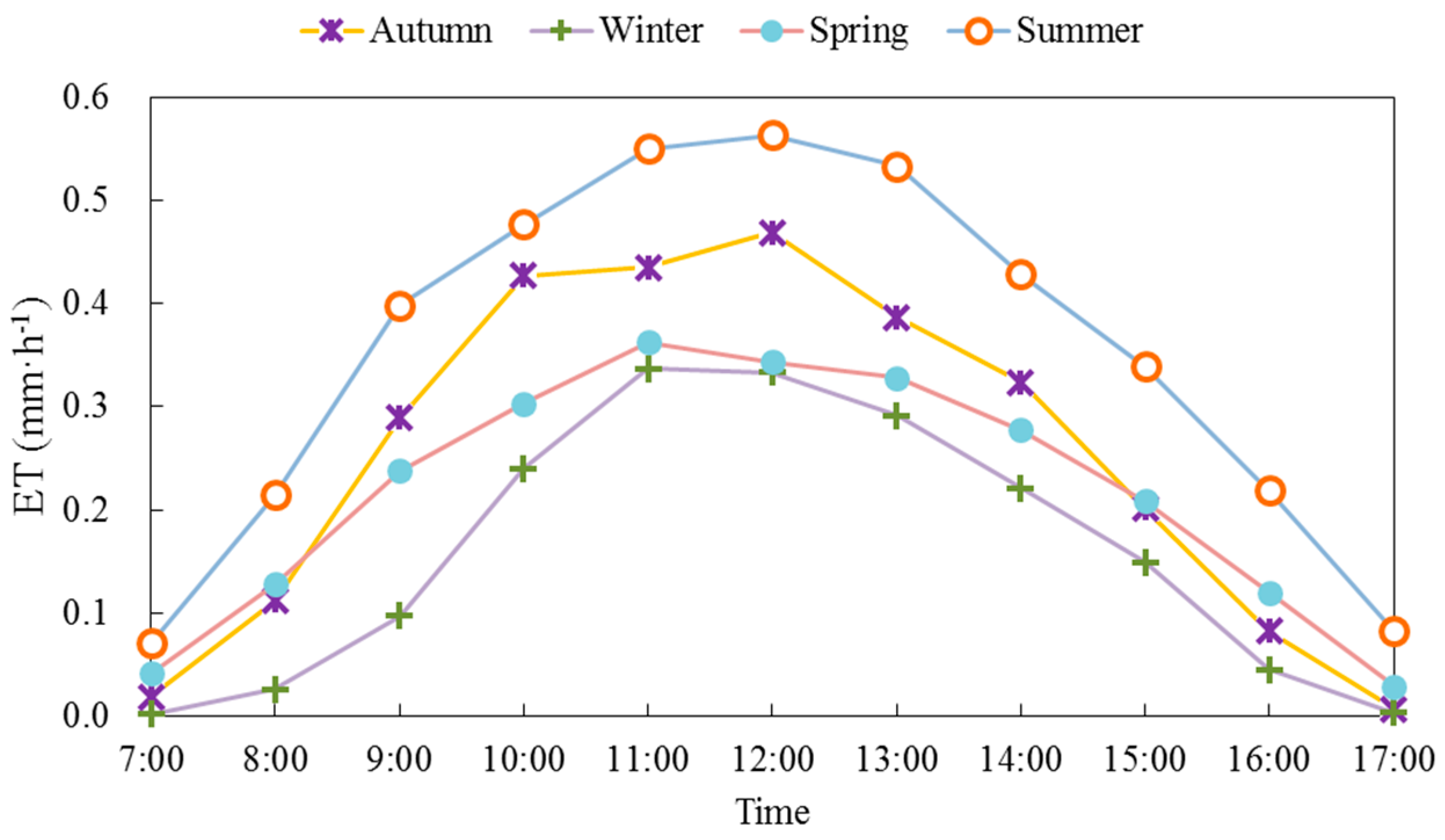
3.2. Magnitude and Variation Trends of Hourly, Daily, and Seasonal ET

As shown in Figure 3, the daily average ET over the year was 2.70 mm (1 October 2014 to 30 September 2015). The maximum daily ET was 6.24 mm (on 3 September 2014), and the minimum daily ET was 0.02 mm (on 12 January 2015). The minimum monthly ET was 42.30 mm (in December) and the maximum monthly value was 128.98 mm (in June). Monthly ET could over 100 mm in the wet season (May to October) but will be less than 60 mm in the dry season (November to March).
We selected one sunny day for each season to analyze the daily variation features of ET. These days were 15 August 2014, 13 October 2014, 16 January 2015, and 16 April 2015, for summer, fall, winter, and spring, respectively. The results are shown in Figure 4. Usually, ET started from 7:00 and tended to zero approximately 17:00. This was due to the four-floor buildings in the east and west of the observation site, which obstructed the sunshine before 7:00 and after the 17:00. It was also shown that ET usually reached its maximum value approximately 11:00–12:00. The daily ET was 5.51, 3.53, 2.80, and 5.08 mm on 15 August, 13 October, 16 January, and 16 April, respectively.
Similar trends were also clearly shown in the seasonal average ET (Figure 5). In summer, the lawn average ET was 0.04 mm h−1 at 7:00, reached a peak of 0.28 mm h−1 at 12:00 and fell to 0.04 mm h−1 at 17:00. ET rates increased dramatically between 7:00–10:00 and remained high through 11:00–13:00. After 14:00, ET rates decreased. Similar results were observed in other seasons.

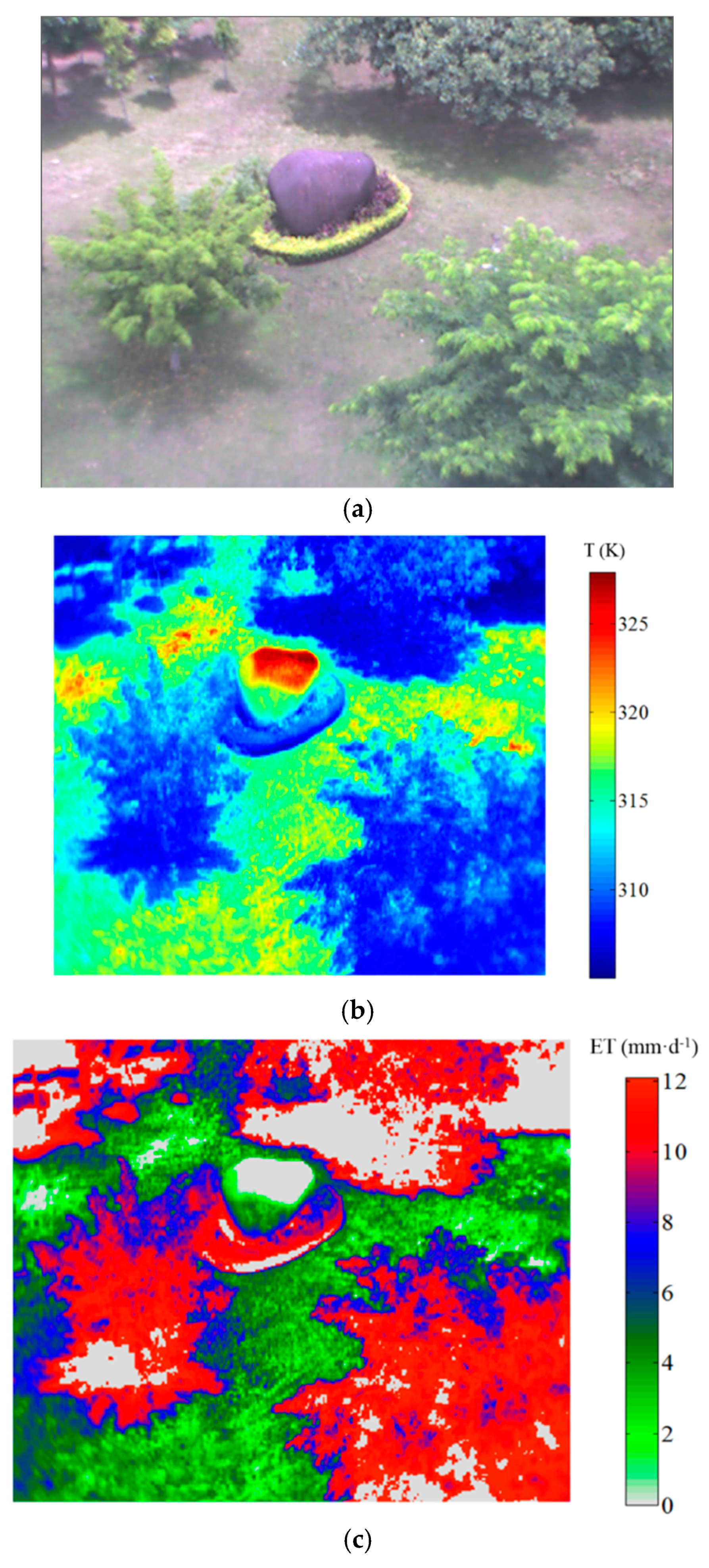
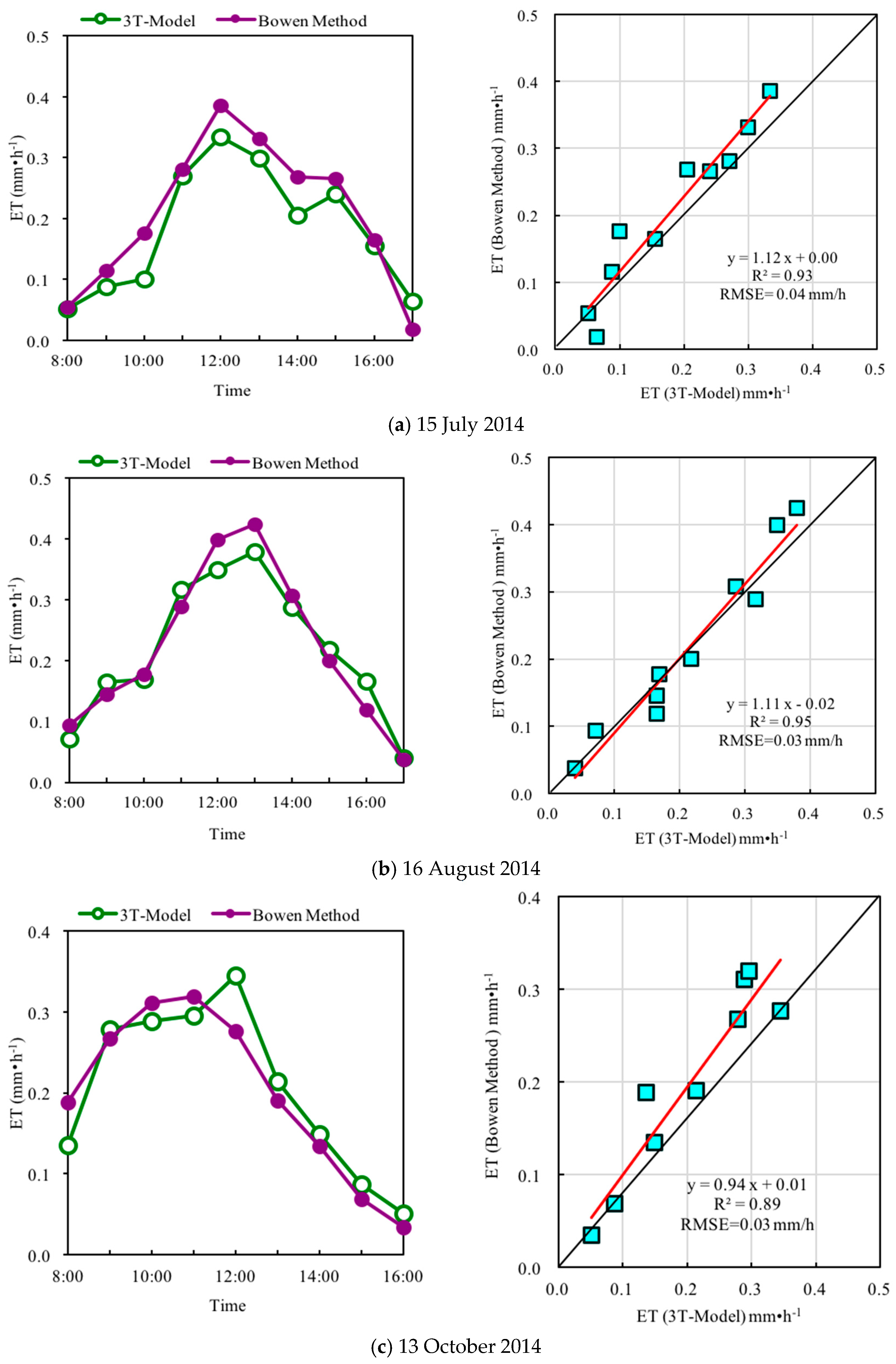
3.3. Urban ET Estimated by ‘3T Model + Infrared RS’ Method

To test this method, measurements carried out over three sunny days (15 July, 16 August, and 13 October 2014) were used as examples (Figure 6 and Figure 7). Figure 6 shows the visible light image, temperature distribution image, and corresponding ET at 12:00 on 15 July 2014. In these images, because we focused only on the ET of lawns (the green area in the lower image), trees, shaded areas, and other areas were not included (the red, blue, and white areas in the bottom image). In the calculation, the measured maximum lawn temperature was used as the reference temperature. According to the same procedures, we obtained the hourly lawn ET on 15 July, 16 August and 13 October. A comparison with the Bowen ratio results is shown in Figure 7.
On 15 July, ET increased from 0.05 mm h−1 at 8:00 to 0.10 mm h−1 at 10:00 and reached the daily peak of 0.33 mm h−1 at 12:00. Then, ET gradually decreased and fell to 0.06 mm h−1 at 17:00. A similar ET trend was observed using the Bowen ratio method. From the scatter diagram (top-right), we found that the results of two methods agreed with each other very well. The distribution of data were close to 1:1 line and the regression line between them was y = 1.12x + 0.03, with a slope close to 1 (1.12), intercept close to zero (0.03), and a high coefficient of determination R2 = 0.93.
Similar trends and results were obtained on 16 August (middle in Figure 7) and 13 October (bottom in Figure 7). On 16 August, the ET rate gradually increased from 8:00 and reached its maximum value at 13:00. On 13 October, the maximum ET value appeared at 12:00. Again, the distribution of data in the two days was close to 1:1 lines. On August 16 and October 13, their regression line and regression coefficient between the ET estimated by the two method was y = 1.11x − 0.24 and Y = 0.98x, R2 = 0.95 and R2 = 0.91 respectively. Their slopes were close to 1 and intercepts were close to zero. The root mean square error was 0.04, 0.03, and 0.03 mm h−1 on 15 July, 16 August, and 13 October 2014, respectively.

4. Discussion

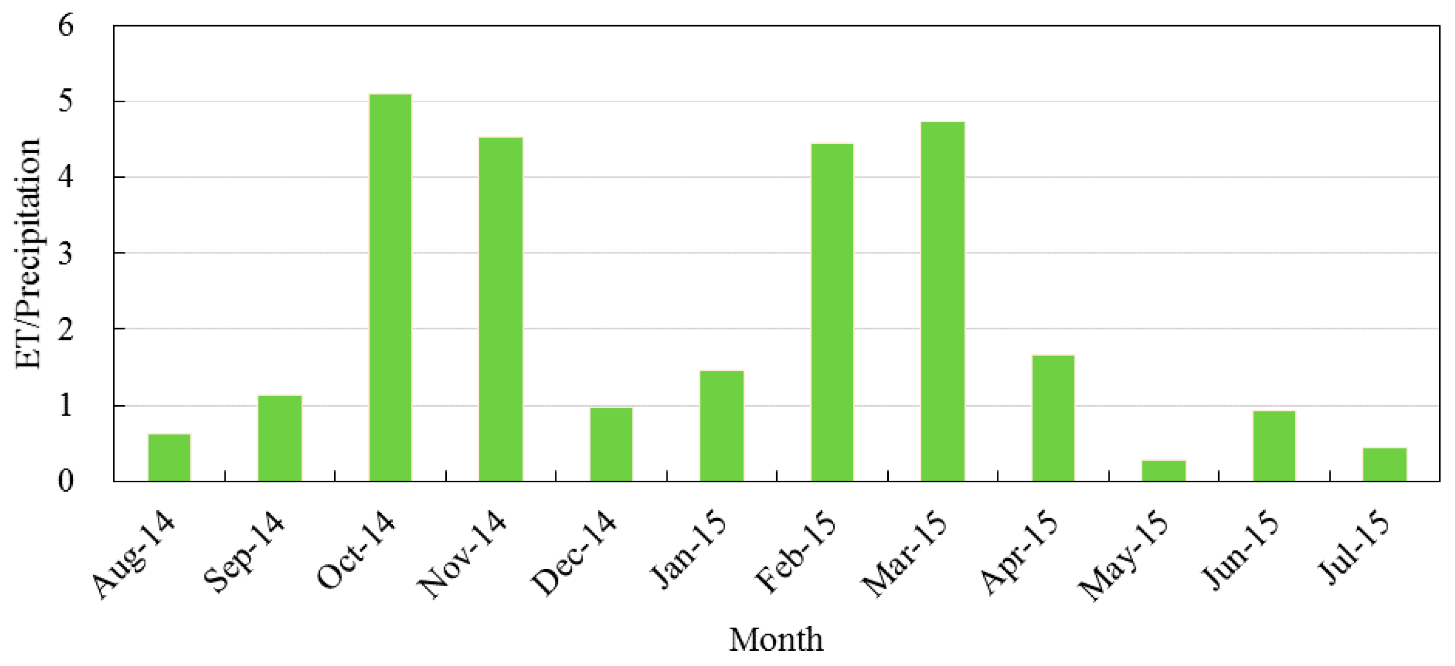
4.1. Relationship between Urban ET and Precipitation (P)

In this study, the daily and monthly ET could reach 6 mm and 100 mm, respectively. Compared with the magnitude of ET observed in other landscapes (grasslands, farmlands, and forests), these values were not small (Yan and Qiu, 2016). The daily ET in our study could reach to 6 mm day−1, much higher than 1–3 mm day−1 observed in other urban areas located in temperate zones [4,29,30]. Urban ET is very obvious and cannot be neglected for water and environmental management.
Though the ratio of ET/P is an important parameter for water management and flood control in urban areas, this ratio is not well known because of a lack of experiment-based ET values. Although there are some urban ET values based on model simulations, the lack of verification makes it difficult to use these poorly tested results. Our results showed that during the whole year (1 August 2014 to 31 July 2015), ET was 361.36 mm and 624.72 mm in the dry and wet seasons, respectively, whereas the corresponding precipitation was 140.20 mm and 1033.10 mm.
As shown in Figure 8, on a monthly basis, ET/P was usually greater than 1 in the dry season (October to March). It was even greater than 4 in October, November, February, and March. However, ET/P was usually less than 1 in the wet season (from April to September). The minimum ET/P was only 0.28 (May).
The average ET/P was 0.6 in the wet season, indicating 60% of precipitation evaporated as vapor. It was 2.6 in the dry season, indicating ET was 260% the precipitation in the same period. The large amount of ET in the dry season was due to added irrigation. Assuming that all rainfall in the dry season was used for lawn ET and the effect of irrigation on ET was not considered, we got ET/P = 0.65 over the year, indicating 65% of the annual precipitation evaporated in this humid city. For many cities located in the sub-humid and sub-arid areas, ET/P could be easily larger than 0.65, indicating most or all of their annual precipitation could be evaporated. There would be less or no surface runoff under these conditions if their vegetation was well established.
As mentioned above, ET could use large amount of solar radiation as latent heat and reduce the air temperature and urban heat island intensity. Our former measurements showed that the ground surface temperature difference between the lawn (with ET) and the nearby paved road (without ET) could be as much as 30 °C in middle summer days [41]. Based on the air temperature measurement at the height of 1.5 m above ground surface, we found that the average urban island intensity could be 1.67 °C lower in this vegetated area than the nearby no vegetation area throughout a two-year period [42]. Furthermore, our results also showed that the daily average transpiration rate (measured by sap-flow method) of a small-sized ficus tree in this field was 36–55 kg (in hot season) and its cooling effect is equivalent to a 1.6–2.4 kWh air conditioner working for all day (24 h) [3]. The cooling effect of ET to urban area and urban heat island is very obvious. Increasing urban ET could be a useful way to mitigate climate warming, especially in urban areas.
Our results revealed that ET can take most of the annual precipitation, even if in a humid subtropical urban environment. This study was one of the very few studies on urban ET based on detailed experiments and observations. This result also showed that vegetation ET can greatly reduce urban runoff, which is important for flood control. In addition, ET can also use a large amount of solar energy and reduce the intensity of urban heat islands. Therefore, Urban ET and E/P are two of the most important parameters for ongoing sponge city design, low impact development, and urban thermal environmental management throughout the world.

4.2. Main Impact Factor of Urban ET

The relationships between ET and meteorological factors have been well studied for years in farmlands, grasslands, forests, and other landscapes. It is clear that there are three main factors controlling ET: the available energy (radiation), vapor diffusion condition (VPD and wind velocity), and soil water availability. However, the main fact controlling urban ET may differ with these landscapes because the lower wind velocity, higher temperature, and lower soil water availability (due to very thin soil layer). This may especially important in our study area because in addition to the lower wind velocity, VPD is lower, too. Therefore, it is interesting to investigate which factor is the most important one to control urban ET. For these purposes, we explored the influence of solar radiation (here we use PAR as representative), air temperature, relative humidity, and wind velocity on ET by using partial correlation analysis method.
We used the average data during a one-year period (1 August 2014 to 31 July 2015) to investigate their relationships. The partial correlation coefficients between urban lawn ET and PAR, relative humidity, wind velocity, and air temperature were 0.927, 0.079, 0.037, and 0.028, respectively, at a 99% confidence level. These results showed that urban ET was strongly related with solar radiation. The relationship between urban ET and relative humidity, wind velocity, and temperature was very weak.
Generally, ET is well related with radiation, humidity, and wind velocity in other landscapes. However, it does not fit with our results. To investigate whether seasonal changes reduced the influence of these factors, we carried out the same analysis using monthly average data. The results are shown in Table 3. Again ET was highly related with PAR with the correlation coefficient varying from 0.65 to 0.92. The correlation coefficients between ET and temperature, humidity, and wind velocity were all very low.
Usually, VPD is an indicator of the combined effect of temperature and humidity. To investigate the effect of VDP on urban ET, we also carried out a partial correlation analysis between ET and PAR, VPD, and wind velocity. The correlation coefficients were 0.923, −0.039, and 0.028, respectively. This result showed that the role of VPD on ET under our conditions was limited.
These results were possibly due to the low wind velocity and constant humidity conditions in the study area. The mean wind velocity in the study site was only 0.3 m s−1 over the experimental period. The daily RH was also stably located in the range of 60% to 80%. Therefore, it was concluded that the urban ET was strongly related only with radiation. The effects of VPD, humidity, temperature, and wind velocity on urban ET were very weak under these urban conditions.

4.3. Evaluation of the ‘3T Model + Infrared RS’ Method for Urban ET Estimation

As discussed before, it is difficult to estimate urban ET by using many of the conventional methods because their fetch requirements cannot be met under the condition of high spatial heterogeneity in urban area. In addition, these methods are usually based on the measurements carried out at one point and then extend its results to the whole field. This also not work under the condition of high spatial heterogeneity in urban areas. In this study, we tried to use the approach of ‘3T model + infrared RS’ to overcome these challenges. We chose this approach because this method does not include wind velocity, VPD, humidity, and other parameters sensitive to spatial heterogeneity. The main input parameter of the proposed method is the surface temperature, which can be measured at over 100,000 points by thermal cameras on the ground, airplanes, and satellites. Up to now, it has been successfully applied under several spatial heterogeneous conditions [43,44,45,46,47,48].
By verifying with Bowen ratio method, it was found that the results of two methods agreed with each other very well. The distribution of ET data were close to 1:1 line, the slope of regression line between them was close to 1 (1.12, 1.11, and 0.98 for the three days, respectively), intercept close to zero (0.03, 0.24, and 0.00 for the three days, respectively), and a high coefficient of determination (R2 = 0.93, 0.95, and 0.91 for the three days, respectively). Urban ET and its spatial heterogeneity can be well measured and revealed by the approach of ‘3T model + infrared RS’. Because wind velocity, VPD, humidity, and other spatial sensitive parameters are not required in this methodology, these advantages make it a suitable methodology for urban ET estimation.

5. Conclusions

The study area is a typical urban area characterized by plenty of sunshine and precipitation, high humidity in the wet season, and a lower wind velocity. These features are very common in subtropical urban and it is worth investigating its ET characteristics. Our studies show that urban ET is mainly affected by solar radiation under these conditions. The effects of air humidity, wind velocity, and air temperature are very weak.
The daily average ET of the urban lawn is 2.70 mm. The average monthly ET in the wet season (May to October) is over 100 mm, whereas it is less than 60 mm in the dry season (November to March). The annual total ET is approximately 990 mm. Compared with the magnitude of ET observed in other landscapes, these ET values are quite obvious. In addition, the average monthly precipitation is 23.37 mm in the dry season and 172.18 mm in the wet season. The ratio of ET/P is 0.65 in the wet season, 2.6 in the dry season, and 0.84 over the year, indicating that ET can take away most of the water from precipitation and much less runoff can be expected. The large amount of ET in the dry season was due to added irrigation. Assuming that all rainfall in the dry season was used for lawn ET and the effect of irrigation on ET was not considered, the ET/P was still 0.65 over the year. This means that 65% of the annual precipitation was evaporated. Urban ET is a highly important component of urban water and energy balances, and it cannot be neglected for sponge city design, low impact development, and urban thermal environmental management.
The fetch-free approach of ‘3T model + infrared RS’ is verified to be a reasonable method to estimate urban ET under highly spatial heterogeneous conditions. The verification results show that the coefficient of determination (R2) of urban lawn ET estimated by the suggested method and Bowen ratio method is greater than 0.93, and the root mean square error is less than 0.04 mm h−1. In addition, the spatial heterogeneity of ET can be reasonably reflected by this approach. Because wind velocity, VPD, humidity, and other spatial sensitive parameters are not required in this method, these advantages make it a suitable methodology for urban ET measurement.

Acknowledgments

We acknowledge, with gratitude, the financial support from the Shenzhen Science and Technology Project (JCYJ20140417144423187, JSGG20150813172407669 and JCYJ20150331160617771) and the Special Fund for Forestry Research in the Public Interest (201304305). The authors would like to express their great thanks to Zhendong Zou, Yongqiang Wang, Longjun Qin, Zhiyuan Niu, Xiaoxue Shen, and others for their assistance in the field experiment of this study. The authors would like to express their great thanks to Elsevier Language Editing for their efforts to improve the grammar of this paper and Tim R. McVicar, Editor of Journal of Hydrology for the advice of submitting.

Author Contributions

Guoyu Qiu designed the research; Shenglin Tan carried out most of the field experiment and data analysis; Xiaohui Yu and Chunhua Yan helped the experiment and data analysis; Guoyu Qiu, Shenglin Tan and Yue Wang wrote the paper.

Conflicts of Interest

The authors declare no conflict of interest.

References

  1. Morini, E.; Touchaei, A.G.; Castellani, B.; Rossi, F.; Cotana, F. The impact of albedo increase to mitigate the urban heat island in Terni (Italy) using the WRF model. Sustainability 2016, 8, 999. [Google Scholar] [CrossRef]
  2. Morini, E.; Castellani, B.; Presciutti, A.; Filipponi, M.; Nicolini, A.; Rossi, F. Optic-energy performance improvement of exterior paints for buildings. Energy Build. 2017, 139, 690–701. [Google Scholar] [CrossRef]
  3. Qiu, G.Y.; Yang, B.; Li, X.; Guo, Q.; Tan, S. Cooling effect of evapotranspiration (ET) and ET measurement by thermal remote sensing in urban. In Proceedings of the AGU Fall Meeting Abstracts, San Francisco, CA, USA, 14–18 December 2015. [Google Scholar]
  4. Grimmond, C.S.B.; Oke, T.R. Evapotranspiration Rates in Urban Areas; IAHS Press: Wallingford, UK, 1999; Volume 259, pp. 235–244. [Google Scholar]
  5. Berthier, E.; Dupont, S.; Mestayer, P.G.; Andrieu, H. Comparison of two evapotranspiration schemes on a sub-urban site. J. Hydrol. 2006, 328, 635–646. [Google Scholar] [CrossRef]
  6. Willems, P. Revision of urban drainage design rules after assessment of climate change impacts on precipitation extremes at Uccle, Belgium. J. Hydrol. 2013, 496, 166–177. [Google Scholar] [CrossRef]
  7. Mancipe-Munoz, N.A.; Buchberger, S.G.; Suidan, M.T.; Lu, T. Calibration of rainfall-runoff model in urban watersheds for stormwater management assessment. J. Water Resour. Plan. Manag. 2014, 140, 05014001. [Google Scholar] [CrossRef]
  8. Grimm, N.B.; Faeth, S.H.; Golubiewski, N.E.; Redman, C.L.; Wu, J.; Bai, X.; Briggs, J.M. Global change and the ecology of cities. Science 2008, 319, 756–760. [Google Scholar] [CrossRef] [PubMed]
  9. Arnfield, A.J. Two decades of urban climate research: A review of turbulence, exchanges of energy and water, and the urban heat island. Int. J. Climatol. 2003, 23, 1–26. [Google Scholar] [CrossRef]
  10. Rossi, F.; Pisello, A.L.; Nicolini, A.; Filipponi, M.; Palombo, M. Analysis of retro-reflective surfaces for urban heat island mitigation: A new analytical model. Appl. Energy 2014, 114, 621–631. [Google Scholar] [CrossRef]
  11. Min, S.K.; Zhang, X.; Zwiers, F.W.; Hegerl, G.C. Human contribution to more-intense precipitation extremes. Nature 2011, 470, 378–381. [Google Scholar] [CrossRef] [PubMed]
  12. Huang, G.R.; He, H.J. Impact of urbanization on features of rainfall during flood period in Jinan city. J. Nat. Disasters 2011, 3, 7–12. [Google Scholar]
  13. Yang, Z.; Dominguez, F.; Gupta, H.V. Urban effects on regional climate: A case study in the Phoenix-Tucson Corridor. In Proceedings of the AGU Fall Meeting Abstracts, San Francisco, CA, USA, 15–19 December 2014. [Google Scholar]
  14. Oke, T.R.; Zeuner, G.; Jauregui, E. The surface energy balance in Mexico City. Atmos. Environ. Part B Urban Atmos. 1992, 26, 433–444. [Google Scholar] [CrossRef]
  15. Grimmond, C.S.B. The suburban energy balance: Methodological considerations and results for a mid-latitude west coast city under winter and spring conditions. Int. J. Climatol. 1992, 12, 481–497. [Google Scholar] [CrossRef]
  16. Grimmond, C.S.B.; Oke, T.R. Turbulent heat fluxes in urban areas: Observations and a local-scale urban meteorological parameterization scheme (LUMPS). J. Appl. Meteorol. 2002, 41, 792–810. [Google Scholar] [CrossRef]
  17. Jim, C.Y.; Chen, W. Assessing the ecosystem service of air pollutant removal by urban trees in Guangzhou (China). J. Environ. Manag. 2008, 88, 665–676. [Google Scholar] [CrossRef] [PubMed]
  18. Jim, C.Y.; Chen, W.Y. Ecosystem services and valuation of urban forests in China. Cities 2009, 26, 187–194. [Google Scholar] [CrossRef]
  19. DiGiovanni, K.; Gaffin, S.; Montalto, F.; Rosenzweig, C. Applicability of classical predictive equations for the estimation of evapotranspiration from urban green spaces: Green roof results. J. Hydrol. Eng. 2013, 18, 99–107. [Google Scholar] [CrossRef]
  20. Voyde, E.; Fassman, E.; Simcock, R. Hydrology of an extensive living roof under sub-tropical climate conditions in Auckland, New Zealand. J. Hydrol. 2010, 394, 384–395. [Google Scholar] [CrossRef]
  21. Ouldboukhitine, S.E.; Andrade, H.; Vaz, T. Assessment of green roof thermal behavior: A coupled heat and mass transfer model. Build. Environ. 2011, 46, 2624–2631. [Google Scholar] [CrossRef]
  22. Neukrug, H. A Triple Bottom Line Assessment of Traditional and Green Infrastructure Options for Controlling CSO Events in Philadelphia’s Watersheds; Philadelphia Water Department and Office of Watersheds: Philadelphia, PA, USA, 2009. [Google Scholar]
  23. Bloomberg, M.; Holloway, C. NYC Green Infrastructure Plan; Office of the Mayor: New York, NY, USA, 2010. [Google Scholar]
  24. Xu, C.Y.; Chen, D. Comparison of seven models for estimation of evapotranspiration and groundwater recharge using lysimeter measurement data in Germany. Hydrol. Process. 2005, 19, 3717–3734. [Google Scholar] [CrossRef]
  25. Bedient, P.B.; Huber, W.C. Hydrology and Floodplain Analysis, 3rd ed.; Prentice-Hall: Upper Saddle River, NJ, USA, 2002. [Google Scholar]
  26. Denich, C.; Bradford, A. Estimation of evapotranspiration from bioretention areas using weighing lysimeters. J. Hydrol. Eng. 2010, 15, 522–530. [Google Scholar] [CrossRef]
  27. Pataki, D.E.; McCarthy, H.R.; Litvak, E.; Pincetl, S. Transpiration of urban forests in the Los Angeles metropolitan area. Ecol. Appl. 2011, 21, 661–677. [Google Scholar] [CrossRef] [PubMed]
  28. Peters, E.B.; Hiller, R.V.; McFadden, J.P. Seasonal contributions of vegetation types to suburban evapotranspiration. J. Geophys. Res. Biogeosci. 2011, 116. [Google Scholar] [CrossRef]
  29. Jacobs, C.; Elbers, J.; Brolsma, R.; Hartogensisc, O.; Moors, E.; María, T.R.M.; Hove, B. Assessment of evaporative water loss from Dutch cities. Build. Environ. 2015, 83, 27–38. [Google Scholar] [CrossRef]
  30. Ward, H.C.; Evans, J.G.; Grimmond, C.S.B. Infrared and millimetre-wave scintillometry in the suburban environment–Part 2: Large-area sensible and latent heat fluxes. Atmos. Meas. Tech. 2015, 8, 1407–1424. [Google Scholar] [CrossRef]
  31. Kim, S.J. Influence of micrometeorological factors for actual evapotranspiration in the coastal urban area. In Proceedings of the AGU Fall Meeting Abstracts, San Francisco, CA, USA, 14–18 December 2015. [Google Scholar]
  32. Litvak, E. Evapotranspiration of the urban forest at the municipal scale in Los Angeles, CA. In Proceedings of the AGU Fall Meeting Abstracts, San Francisco, CA, USA, 14–18 December 2015. [Google Scholar]
  33. Miller, G.R.; Long, M.R.; Fipps, G.; Swanson, C.; Traore, S. Spatiotemporal variability in potential evapotranspiration across an urban monitoring network. In Proceedings of the AGU Fall Meeting Abstracts, San Francisco, CA, USA, 14–18 December 2015. [Google Scholar]
  34. Nouri, H.; Nagler, P.L. Evapotranspiration estimation in heterogeneous urban vegetation. In Proceedings of the AGU Fall Meeting Abstracts, San Francisco, CA, USA, 14–18 December 2015. [Google Scholar]
  35. Lazzarin, R.M.; Castellotti, F.; Busato, F. Experimental measurements and numerical modelling of a green roof. Energy Build. 2005, 37, 1260–1267. [Google Scholar] [CrossRef]
  36. Bowen, I.S. The ratio of heat losses by conduction and by evaporation from any water surface. Phys. Rev. 1926, 27, 779–789. [Google Scholar] [CrossRef]
  37. Andreas, E.L.; Cash, B.A. A new formulation for the Bowen ratio over saturated surfaces. J. Appl. Meteorol. 1996, 35, 1279–1289. [Google Scholar] [CrossRef]
  38. Pauwels, V.R.N.; Samson, R. Comparison of different methods to measure and model actual evapotranspiration rates for a wet sloping grassland. Agric. Water Manag. 2006, 82, 1–24. [Google Scholar] [CrossRef]
  39. Qiu, G.Y.; Momii, K.; Yano, T. Estimation of plant transpiration by imitation leaf temperature. I. Theoretical consideration and field verification. Trans. Jpn. Soc. Irrig. Drain. Reclam. Eng. 1996, 64, 47–56. [Google Scholar]
  40. Yan, C.; Qiu, G.Y. The three-temperature model to estimate evapotranspiration and its partitioning at multiple scales—A review. Trans. ASABE 2015, 59, 661–670. [Google Scholar]
  41. Yang, Y.; Zou, Z.; Zhao, W.; Li, R.; Qiu, G.Y. The study of optical properties and thermal performance of thin layer concrete pavement commonly used in the urban environment’s external surface. Ecol. Environ. Sci. 2016, 25, 835–841, (In Chinese with English Abstract). [Google Scholar]
  42. Li, X.; Li, H.; Zhang, Q.; Qiu, G.Y. Study on reducing effect of different urban landscapes on urban temperature. Ecol. Environ. Sci. 2014, 23, 106–112, (In Chinese with English Abstract). [Google Scholar]
  43. Qiu, G.Y.; Omasa, K.; Sase, S. An infrared-based coefficient to screen plant environmental stress: Concept, test and applications. Funct. Plant Biol. 2009, 36, 990–997. [Google Scholar] [CrossRef]
  44. Song, L.; Liu, S.; Zhang, X.; Zhou, J. Estimating and validating soil evaporation and crop transpiration during the HiWATER-MUSOEXE. IEEE Geosci. Remote Sens. Lett. 2015, 12, 334–338. [Google Scholar] [CrossRef]
  45. Qiu, G.Y.; Zhao, M. Remotely monitoring evaporation rate and soil water status using thermal imaging and “three-temperatures model (3T Model)” under field-scale conditions. J. Environ. Monit. 2010, 12, 716–723. [Google Scholar] [CrossRef] [PubMed]
  46. Xiong, Y.J.; Qiu, G.Y. Simplifying the revised three-temperature model for remotely estimating regional evapotranspiration and its application to a semi-arid steppe. Int. J. Remote Sens. 2014, 35, 2003–2027. [Google Scholar]
  47. Tian, F.; Qiu, G.Y.; Lü, Y.H.; Yang, Y.H.; Xiong, Y. Use of high-resolution thermal infrared remote sensing and “three-temperature model” for transpiration monitoring in arid inland river catchment. J. Hydrol. 2014, 515, 307–315. [Google Scholar] [CrossRef]
  48. Wang, Y.Q.; Xiong, Y.J.; Qiu, G.Y.; Zhang, Q.T. Is scale really a challenge in evapotranspiration estimation? A multi-scale study in the Heihe oasis using thermal remote sensing and the three-temperature model. Agric. For. Meteorol. 2016, 230–231, 128–141. [Google Scholar] [CrossRef]
Figure 1. Location of the study area. The upper left figure shows the location of Shenzhen city in China. The upper right figure shows the location of experimental field in Shenzhen. The bottom left figure shows the experimental field and the location of Bowen ratio system (scale = 1:12,500). The photo at bottom right is the Bowen ratio system tower and the lawn field.
Remotesensing 09 00502 g001
Figure 2. (af) Daily mean value of solar radiation (Rs), net radiation (Rn), photosynthetic active radiation (PAR), air temperature, relative humidity, precipitation, and wind velocity over the period (from 11 July 2014 to 30 September 2015) in the experimental site.
Remotesensing 09 00502 g002aRemotesensing 09 00502 g002b
Figure 3. Daily (a) and monthly (b) average ET of the urban lawn from 11 July 2014 to 30 September 2015. Data were measured using the Bowen ratio tower.
Remotesensing 09 00502 g003
Figure 4. Diurnal variations of lawn ET on typical sunny days in the four seasons in Shenzhen. 15 August 2014, 13 October 2014, 16 January 2015, and 16 April 2015 represent summer, fall, winter, and spring, respectively.
Remotesensing 09 00502 g004
Figure 5. Diurnal variations of seasonal average ET of lawn in the four seasons.
Remotesensing 09 00502 g005
Figure 6. Visible light image (a), temperature image (b), and ET of a lawn (c) at 12:00 on 15 July 2014. ET was estimated by infrared RS + 3T model method. Images were taken almost vertically from a tower approximately 50 m high.
Remotesensing 09 00502 g006
Figure 7. (ac) Comparison of the lawn ET estimated using the ‘infrared RS + 3T model’ and Bowen ratio method.
Remotesensing 09 00502 g007
Figure 8. Ratio of ET to precipitation in different months over a one-year period.
Remotesensing 09 00502 g008
Table 1. Type of sensor, measurement height, and resolutions of the equipment in Bowen ratio system.
ParameterSensor TypeMeasuring Height (m)Sensor Resolution
Humidity & temperature225-050YA, Novalynx, Grass Valley, CA, USA2.0; 1.5±3%, ±0.6 °C
Wind velocity & direction200-WS-02, Novalynx, Grass Valley, CA, USA2.0±0.2 m s−1, ±3°
Solar radiationPYP-PA, Apogee, Santa Monica, CA, USA2.010–40 μV/W/m2
Photosynthetic active radiationQSOA-S, Apogee, Santa Monica, CA USA2.0<3%
Net radiation240-100, Novalynx, Grass Valley, CA, USA2.0<4%
Soil heat fluxHFP01, Hukseflux, Center Moriches, NY, USA−0.05; −0.0250 μV/W/m2
Table 2. Monthly mean value of the meteorological parameters in the study area.
Temperature (°C)Humidity (%)Solar Radiation (W m−2)Net Radiation (W m−2)PAR (μmol m−2 s−1)Wind Velocity (m s−1)
2014August29.5478.05338.37114.50811.670.20
September28.7178.76328.7299.55742.480.15
October25.8467.69330.9487.70752.030.14
November22.4369.74218.7348.85512.170.13
December15.0261.05185.5630.16410.660.13
2015January15.4663.31255.5547.21593.470.18
February17.9561.27229.0652.06534.660.23
March20.9966.51189.8551.55454.870.23
April23.7360.19267.5775.51600.840.25
May27.8963.81244.5487.11593.970.34
June30.2057.10350.27134.23825.460.34
July29.5058.25296.17111.68717.600.24
August29.2460.31331.55112.52789.940.12
September28.4259.37324.2397.43768.370.12
Table 3. Partial correlation coefficients between the urban lawn ET and air temperature, relative humidity (RH), PAR, and wind velocity in different months over the experimental period.
MonthTemperatureRHPARWind Velocity
August 20140.2570.2440.6530.194
September 20140.0340.0180.917−0.182
October 20140.105−0.0060.7920.307
November 2014−0.157−0.1300.758−0.012
December 20140.079−0.0230.665−0.092
January 2015−0.289−0.2630.7720.157
February 20150.0140.0460.784−0.225
March 2015−0.087−0.0310.8500.158
April 2015−0.157−0.0930.8920.067
May 20150.5980.5820.885−0.316
June 2015−0.072−0.0220.862−0.028
July 2015−0.255−0.2720.7690.045
August 2015−0.213−0.2290.815−0.161
September 2015−0.275−0.2730.764−0.121

