Abstract
Inhomogenities in the sea ice motion field cause deformation zones, such as leads, cracks and pressure ridges. Due to their long and often narrow shape, those structures are referred to as Linear Kinematic Features (LKFs). In this paper we specifically address the identification and characterization of variations and discontinuities in the spatial distribution of the total deformation, which appear as LKFs. The distribution of LKFs in the ice cover of the polar oceans is an important factor influencing the exchange of heat and matter at the ocean-atmosphere interface. Current analyses of the sea ice deformation field often ignore the spatial/geographical context of individual structures, e.g., their orientation relative to adjacent deformation zones. In this study, we adapt image processing techniques to develop a method for LKF detection which is able to resolve individual features. The data are vectorized to obtain results on an object-based level. We then apply a semantic postprocessing step to determine the angle of junctions and between crossing structures. The proposed object detection method is carefully validated. We found a localization uncertainty of 0.75 pixel and a length error of 12% in the identified LKFs. The detected features can be individually traced to their geographical position. Thus, a wide variety of new metrics for ice deformation can be easily derived, including spatial parameters as well as the temporal stability of individual features.
1. Introduction
The drift of sea ice is mainly driven by atmospheric and oceanographic forcing. The stress exerted on the ice is caused by variations in the acting forces and by blocking effects occuring along coastlines or at obstacles such as islands, icebergs, and fast ice. The internal forces trigger the formation of deformation structures such as leads, cracks, pressure ridges, hummocks and rubble fields. Leads, for instance, are elongated openings in the ice cover caused by divergent ice motion. They influence the exchange of heat and matter at the ocean-atmosphere interface, are locations of new ice formation, and decrease the local albedo. The knowledge of their position is also valuable for ship routing. Ridges and rubble fields, on the other hand, indicate the action of compressional forces. They increase the variability of the ice thickness, influence the interactions between atmosphere, ice, and ocean, and affect marine operations in the polar regions. The spatial distribution and orientation of deformation structures indicates material properties of the sea ice [1,2]. The adequate implemetation of sea ice rheology, which describes the internal forces in the ice, is crucial for the ability of coupled ice-ocean models to realistically simulate ice dynamics [3]. Deformation structures are often denoted by the term “linear kinematic feature” (LKF), since they all are highly localized in their width and appear on length scales ranging from several kilometers to hundreds of kilometers [4,5].
Deformation features may be characterized by different quantitative parameters, some of which can be derived from images acquired from satellite or airborne platforms. The first step is to detect and separate different structures in the images. Several studies have been focused on lead and ridge detection. Onana et al. [6] and Willmes et al. [7], e.g., used thermal infrared images to study the arctic-wide lead distribution. Lindsay et al. [8] and Bröhan et al. [9] presented methods for detecting arctic sea ice leads in radiometer data, while [10] used optical/thermal imagery for this purpose. An important aspect of those studies was the determination of lead orientation and fraction. Vesecky et al. [11] described a method for extracting leads and ridges in spaceborne and airborne Synthetic Aperture Radar (SAR) images. The objectives were to determine ridge lengths and orientation and compare results obtained from images acquired at different radar frequencies [12]. Also using airborne SAR images, Dierking, W. et al. [13] derived thresholds for separating deformed and level ice. They investigated the potential of different radar frequencies and polarizations for the detection of deformation zones and the determination of their areal fraction together with the size distribution of level ice floes between them. Dierking et al. [13] presented an object-based ridge detection scheme that they applied to high-resolution rasterized aerial photographs to retrieve ridge frequency, length and height from the area of the shadows cast by the ridges. We emphasize here that those studies focused on intensity variations in the images.
Instead of using SAR intensity imagery, we focus specifically on patterns in the sea ice deformation field for the entire Arctic region, hence directing our attention to large scale LKFs (lead systems, zones of convergence) reaching over several hundred kilometers. The motivation was to establish a method for comparing results of sea ice model simulations with corresponding information retrieved from from temporal sequences of SAR images. Here, we concentrate on patterns of total deformation, but our method can be applied to any data that reveal spatial patterns (e.g., intensity images, drift velocity fields).
This paper is structured in the following way: Section 2 introduces the data used for the development of the object detection method and describes the different steps of processing. The results are shown and validated in Section 3. We discuss our findings in Section 4. The key points of this study are summarized in Section 5.
2. Methods
2.1. Data
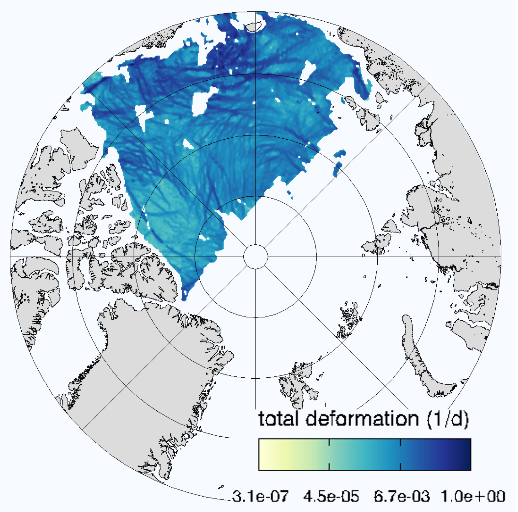
Development and testing of the algorithm was carried out based on the RGPS (Radarsat Geophysical Processor System) sea ice deformation product [14], since it is publicly available and easy to handle. The RGPS product has a spatial resolution of 12.5 km and the intervals between observations range from 1.5 h (one orbit) to 15 days. It is gridded on a polar stereographic projection with the central meridian at +70° and a −45° standard parallel [15], and is defined on an Eulerian grid [16]. The dataset used here (Figure 1) covers the entire year 2006. As already mentioned above, our algorithm detects LKFs based on the spatial variations of total deformation. This parameter is not available as a RGPS product, but can be easily computed from divergence and shear [17]. Possible issues arising due to the presence of outliers and quantization noise in the RGPS data are not considered here, since our development of an object-based detector for interrelated linear features does not include preprocessing steps for increasing the quality of the used data set. A possible preprocessing step could for example be based on the calculation of ice deformation as proposed in [18].

Figure 1.
RGPS (Radarsat Geophysical Processor System) example data set (4 January 2006), calculated total deformation.
2.2. Image Enhancement, Segmentation and Edge Detection
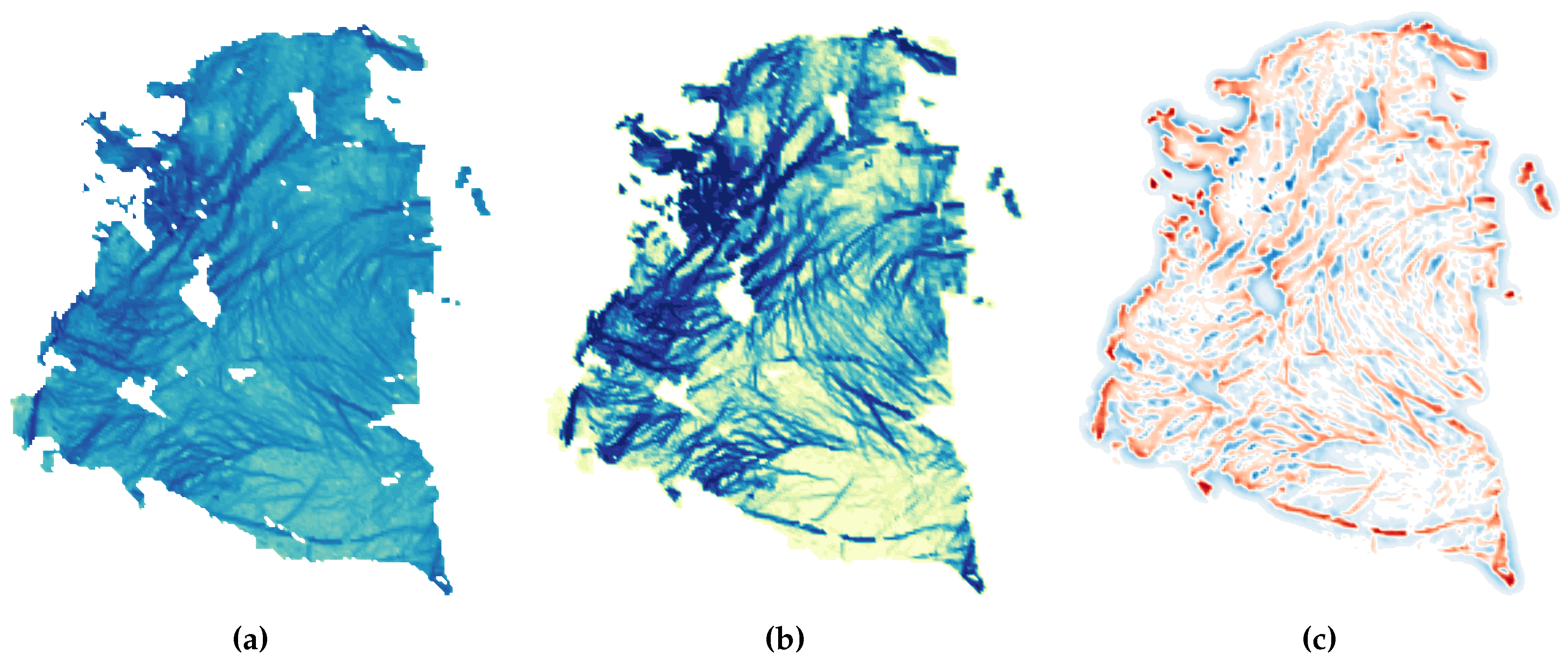
This study aims to detect smaller, less pronounced deformation structures besides regions of high deformation, trying to include as many deformation features on different spatial scales as possible. Sea ice deformation is spatially very heterogeneous, and the distribution of the deformation energy exhibits multi-fractal properties [19]. It is noted in [20] that the determination of thresholds for strain rate values (needed to define LKFs) is a scale-dependent procedure. Therefore, a simple threshold-based LKF detection approach was not considered suitable. Instead, the total deformation data is processed using the following image processing steps. First, the visibility of the weaker deformation zones is enhanced by logarithmic scaling of the total deformation as follows: . Figure 2a shows the scaled result, . The contrast in the resulting image is additionally increased by histogram equalization (Figure 2b). Note that the samples of image processing steps shown in Figure 2 correspond to the studied ice region shown in Figure 1.

Figure 2.
Image enhancement: (a) Logarithm-scaled total deformation ; (b) Result of histogram equalization; (c) DoG (Difference of Gaussian) filtered image. red: , blue: .
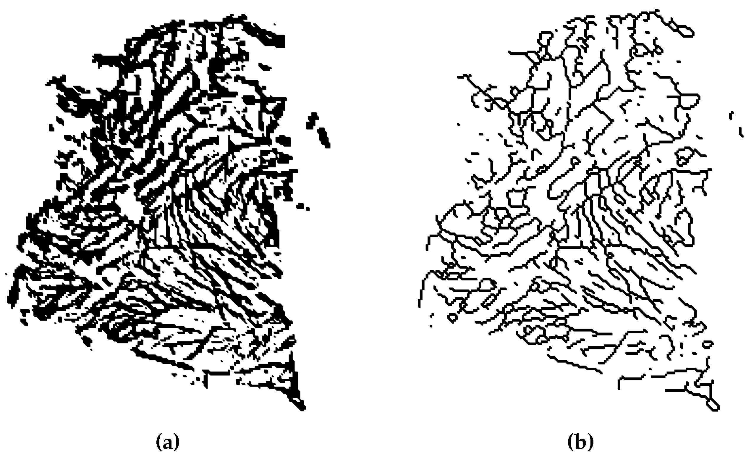
In the next step, the deformation features need to be separated from the background, and this can be treated as a classic edge detection problem. Most edge detection methods determine edge location by calculating the spatial derivatives of the image [21]. The maximum of the 1st derivative and zero-crossing of the 2nd derivative then indicate the position of the edges in the image [22]. Images of natural scenes often show objects at different spatial scales. Therefore, edge detection algorithms applied to natural images need to account for the size distribution of the depicted objects. Among other studies, the one described in [23] suggests a multiscale approach to detect edges of objects in natural scenes. Filters with different kernel sizes were used to enhance edges at different spatial scales. The most significant length scales are then obtained through a weighting function for the cumulative edge strength. In [24], a linear combination of gradients calculated at different spatial scales is used to to detect edges. The present study follows these scaling the approaches. We use the Difference of Gaussian (DoG) filter in a linear combination of different kernel sizes to account for different object scales. A DoG filter acts as a bandpass filter which suppresses small-scale noise and also large-scale components representing the homogeneous areas in the image. The frequency components in the passing band are associated with the edges in the image. An extensive discussion of DoG filtering can be found in [25]. Starting with the result of the histogram equalization (Figure 2b), the filtered image is calculated as from the individual DoG filtering results, , with kernel sizes of . The different kernel sizes correspond to different spatial scales. The result of the filtering operation can assume positive and negative values. It is shown in Figure 2c. The maximum values of the total deformation are isolated by the next two processing steps: first, by segmenting to obtain the binary representation (shown in Figure 3a):

Figure 3.
Image segmentation: (a) Segmentation result ; (b) Result of thinning B.
Morphological thinning (see [26] for a detailed description) as the second step reduces the segmented features to center lines of one pixel width to obtain image B (Figure 3b) as the final result of the edge detection.
2.3. Object Detection
The segmentation and thinning steps result in a binary representation of the LKF locations. At this point, it is not possible to analyze the data on the level of individual LKF objects. This requires an additional layer of abstraction, and some prior knowledge about the image content. Sea ice deformation is characterized by the presence of highly localized linear features which may intersect each other due to successively occurring fracture events which are, in turn, caused by spatially varying forcing conditions. Most objects that we deal with have the following properties: (1) they are linear (elongated) features; (2) they exhibit a low curvature and no abrupt change of direction; (3) they are not closed (circular); and (4) objects are allowed to arbitrarily branch or intersect. Many out-of-the-box object detection approaches are optimized to detect closed shapes and explicitly avoid intersections [25]. Hence they are not suitable in our case. An alternative is to look at road network detection techniques [27,28,29], but the approaches taken there are fairly complex due to the need to separate all non-road-related information.
For the detection of sea ice deformation structures, no such issues are encountered since we only need to separate LKFs from the patches between them, and a more basic approach can be used. According to Equation (1), the segmented LKF’s assume values of 1, while the background is set to 0. Due to the condition of linearity, it is convenient to represent each detected object as a polyline (a set of two-dimensional points defined on the image coordinate system). With those premises, a relatively simple line-following algorithm on B can be implemented which evaluates the 8-neighborhood of each pixel at position , where .
Finding the starting points of possible objects in the thinning result B is straightforward, since the sum of all pixels with in the 8-neighborhood always equals 2 (Figure 4a). At such a point, a new object is created and the coordinates of the starting point are stored. As long as the sum over B of the 8-neighborhood equals 3, a running box moves along the direction of the line. At each direction change, a new vertex containing the point coordinates is added to the object (Figure 4b). An intersection is encountered if the sum exceeds 3 (Figure 4c). In this case, the box is moved following the direction of the lowest curvature, taking the line history into account.
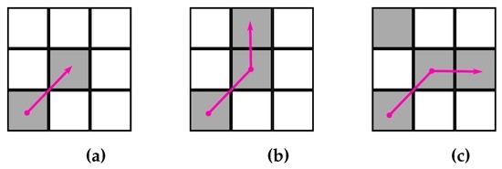
Figure 4.
Example neighborhoods/detection steps. The magenta lines symbolize detected polyline objects. (a) Line start; (b) Direction change; (c) Intersection.
The prior knowledge of the image content requires linear structures, and strong direction changes often imply the start of a different LKF. For this reason, the polyline will end if its direction changes by more than 45° compared to its previous segment. Otherwise, the line ends if the sum over the neighborhood falls below 2. This process is repeated until all possible lines contained in B have been detected. The result of this processing step is a set of objects, with each object containing a list of line vertices.
2.4. Semantic Postprocessing
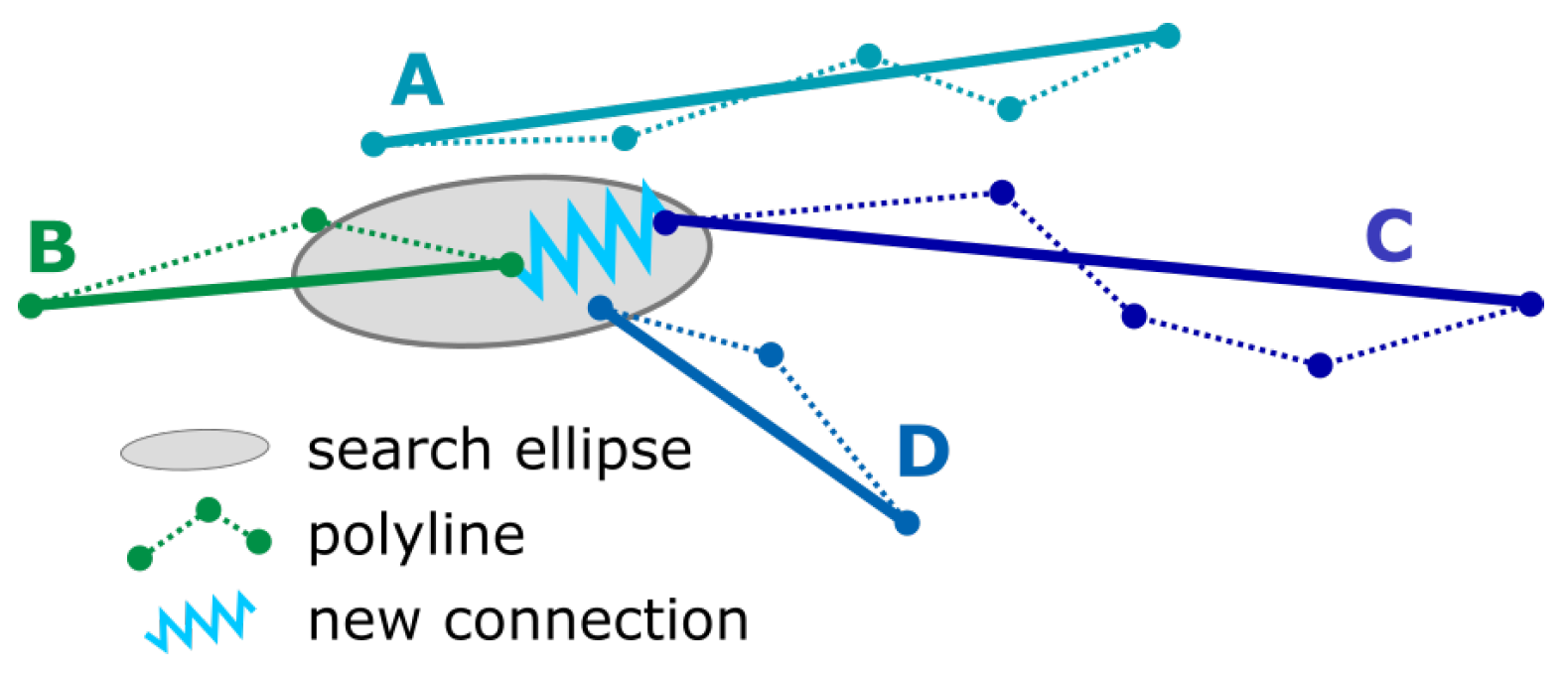
The detected polylines are often broken into smaller segments which need to be reconnected, but this process can be ambiguous. In Figure 5, for instance, lines B and C probably belong to one single object and could thus be connected, whereas A and B appear to be separate features which run in parallel. Even though D is closest to B, it would be considered to be a separate object due to the large orientation difference relative to B.
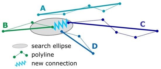
Figure 5.
Example for demonstrating the problem of connecting adjacent LKFs. Dotted lines indicate single segments of the real LKF, the solid lines represent the major orientation of the LKF. In the search ellipse, the end point of line B can potentially be connected to line C or D. The decision is based on differences between the major orientations.
Hence, it becomes necessary to “understand” the information contained in the detected objects by evaluating their context. To this purpose, a basic set of semantic rules is established, similar to [30]. Line segments are connected to each other if they fulfill two criteria: the orientation difference of the two segments needs to be within a tolerable range and the distance between the end points must be within an acceptable limit. Those criteria are implemented as follows:
- Calculate the angle for each object i from a line connecting the polyline endpoints and normalize to orientation: . Hence, the entire polyline (rather than single polyline segments) is used to obtain the general object orientation.
- For each object i, select the set L of objects j which have a similar orientation . The limit of 35° was chosen based on investigations of the data, a more detailed description is given in the Appendix A. The value introduced here allows to tolerate a small degree of curvature in the detected objects. In the example above, L would include lines A and C, if B was used as the reference object.
- Transform each object , to a local coordinate system with the -axis parallel to i and the origin at the start point of i, .In the practical implementation, the positions of matching candidates j with respect to the reference object i are not known. For each object i, a maximum of two objects and can be found which can be attached to the start- or the end segment of i.
- Now we apply anisotropic scaling to compress objects i and j along the – axis. In this way, we implement different search tolerances in and in direction to avoid connections between close parallel lines. The scaled coordinates are now:In the example shown in Figure 5, this would rule out line A and leave line C to be (correctly) connected to B.
- Calculate the endpoint distance . If is below a user-defined threshold, objects i and j are concatenated.
At this point in the post-processing chain it is safe to remove remnant noise in the shape of unconnected small line segments. The minimum size of the detected objects, , can be adjusted by the user, and objects with a length of less than are discarded. The object length is determined by counting the pixels.
The detected lines are subject to discretization noise from the resolution of the input data. As a result, the retrieved objects are not smooth linear features but have a jagged, edgy appearance. In the last post-processing step, they are smoothened by fitting splines to the detected vertices, using the parametric cubic spline interpolation approach described in [31] (Figure 6).
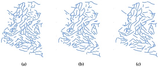
Figure 6.
Detected objects, different minimum length and number of detected objects n. (a) = 4 px, n = 208; (b) = 6 px, n = 160; (c) = 8 px, n = 124.
3. Results and Validation
Figure 6 shows the object detection results for different minimum feature lengths px. A higher results in a stronger generalization of the resulting objects, producing smoother and fewer features. A visual comparison with the original deformation image (Figure 2a) indicates that the most salient deformation strucutures are detected by our method.
3.1. Validation with Reference Data
Independent field data to validate the results of the object detection does not exist. One possibility, though, is to compare the results to lines picked by hand. Even though this method is subjective, studies on large datasets of manually segmented natural scenes found that the most salient image features are reliably detected [32]. In this study, two extensive sets of hand-picked linear features were generated for validation purposes. The visual detection was in all cases based on the log-scaled total deformation (see Figure 2a). The deformation features are in most cases well localized and relatively easy to trace, but ambiguities due to the subjectivity of the human observer still exist. Judging from experience, the largest error source in the reference data sets originates from inaccuracies in the detection of the start- and endpoints.
For a methodically sound validation, it is necessary to evaluate the intrinsic accuracy of the hand-picked lines first. To this purpose, the visual line detection for all LKFs within one single RGPS image was repeated seven times. This dataset contains 1258 polyline objects in total. The resulting set of data is shown in Figure 7a and will be referred to as . The zoom-in (Figure 7b) demonstrates the difficulties to precisely determine the position and length of single segments in an LKF on pixel-scale.
Figure 7.
Intrinsic accuracy of the validation data. (a) Reference features in . The yellow box marks the location of Figure 7b; (b) Reference line example. Hatched area: mean value ± standard deviation of the seven individually determined results from the data set (dashed white lines).
For checking whether there is a systematic bias between all hand-picked and the automatically detected LKFs, each of the latter was combined with the corresponding manually detected seven LKFs into another data set . Any systematic difference between the automatically identified and manually derived LKFs shows up when comparing the and dataset.
A second reference data set () was built to independently evaluate the object detection by picking all visible linear features in 10 RGPS images, but in this case the manual identification of each LKF was only carried out one time. In total, 1411 polyline objects are detected by visual tracking. For the same set of RGPS images, the automated method with = 7 px finds 1647 objects. Choosing a high value causes a relatively strong generalization of the detected features. This behaviour replicates the detection bias apparent in the visual tracking results by favoring longer features which appear to be more significant to the human observer [33]. The factor was hence adapted to approximately match the number of visual detection results.
For all reference datasets, the line detection accuracy was calculated by evaluating pairs of corresponding objects and then determining the error distribution function for all available samples. The error estimates listed below are based on the maximum of the respective error distribution function.
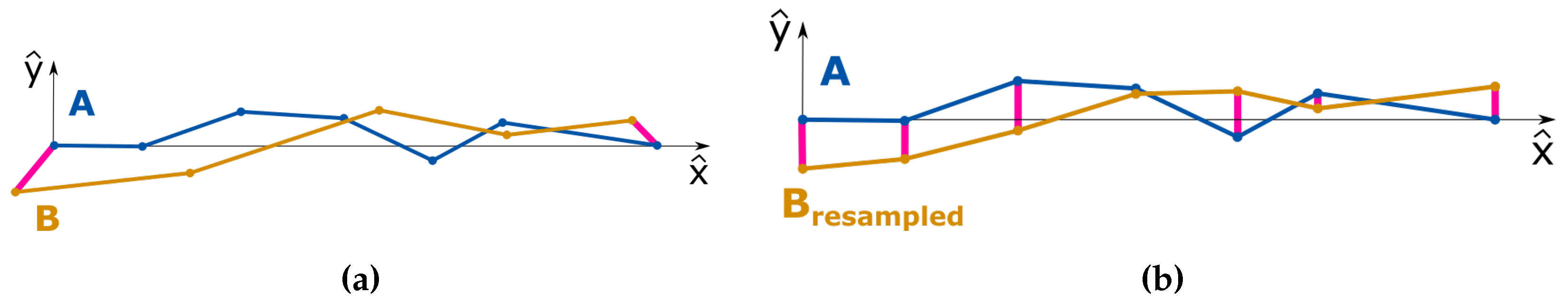
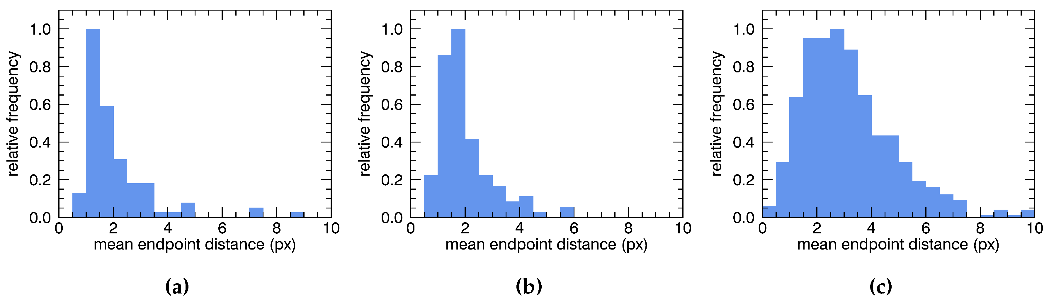
To quantify the line detection accuracy, the set of corresponding polyline objects is transformed to the local -system using Equation (2). The mean absolute distance between start- and endpoints of the detected and the reference LKF is then used to quantify the error in positioning the ends of each LKF, as shown in Figure 8a. The normalized error distribution function for the mean endpoint distances in all evaluated test cases is shown in Figure 9. In the following figures, N denotes sample size, and is the mode of the error distribution function.
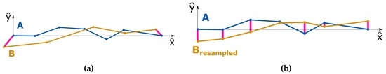
Figure 8.
Uncertainties in LKF localization. (a) Endpoint deviation = average of the lengths of the two magenta lines connecting the endpoints of lines A and B ; (b) Contributions to the localization error (magenta lines). Since A and B are sampled at different -positions, line B is interpolated at the -positions of line A. The interpolated line is denoted B in the figure.

Figure 9.
Distribution of mean endpoint distances. (a) : N = 129, = 1.75 px; (b) : N = 136, = 1.25 px; (c) : N = 1411, = 2.75 px.
The error distribution functions exhibit the log-normal behaviour typical of natural processes with a lower limit (which is in this case due to the spatial resolution limit of the RGPS data). The distributions based on the and datasets (Figure 9a,b) are almost identical, with standard deviations of approximately 1.75 px and 1.25 px (21.88 and 15.3 km), respectively. The standard deviation derived from the dataset is larger, with = 2.75 px (34.4 km) (Figure 9c).
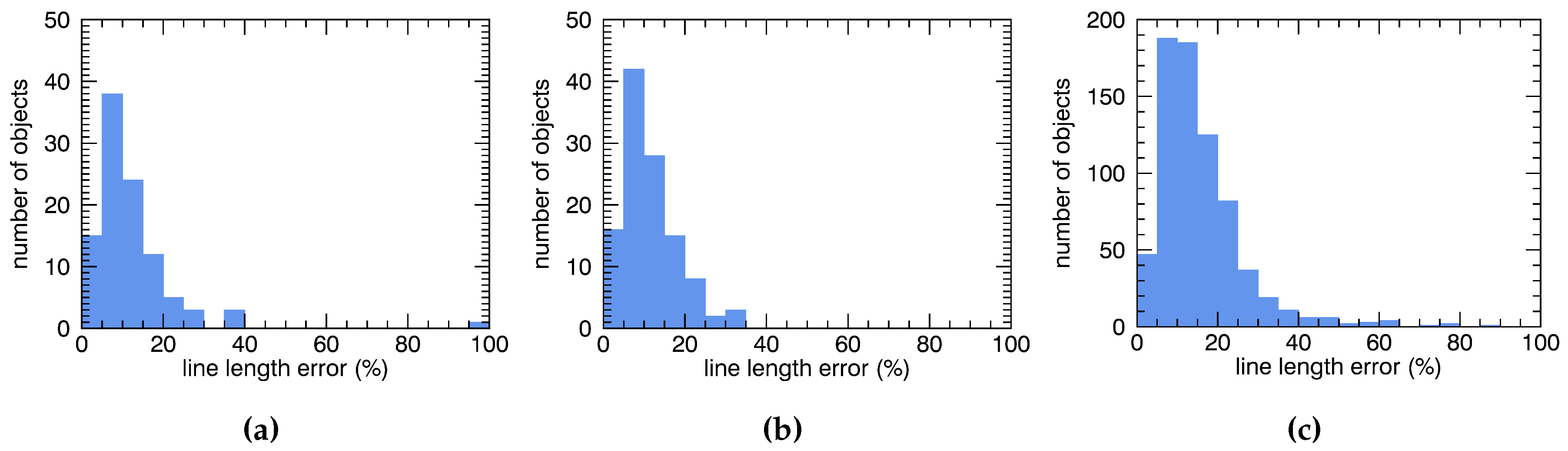
In a second step, we investigate how the length error behaves with respect to absolute line length. To avoid errors introduced by the map projection, we determine the LKF length based on geographical coordinates, i.e., the arc lengths on the reference ellipsoid of each polyline segment are calculated and then integrated over all segments to give the total LKF length. For all investigated cases, the distribution functions are shown in Figure 10. The error values derived from the distribution maxima are on the order of 8% for the - and - data, and 12% in the case.
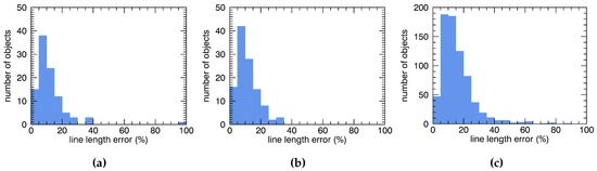
Figure 10.
LKF length error distribution (in percent of the total line length). (a) : N = 129; (b) : N = 136; (c) : N = 1411.
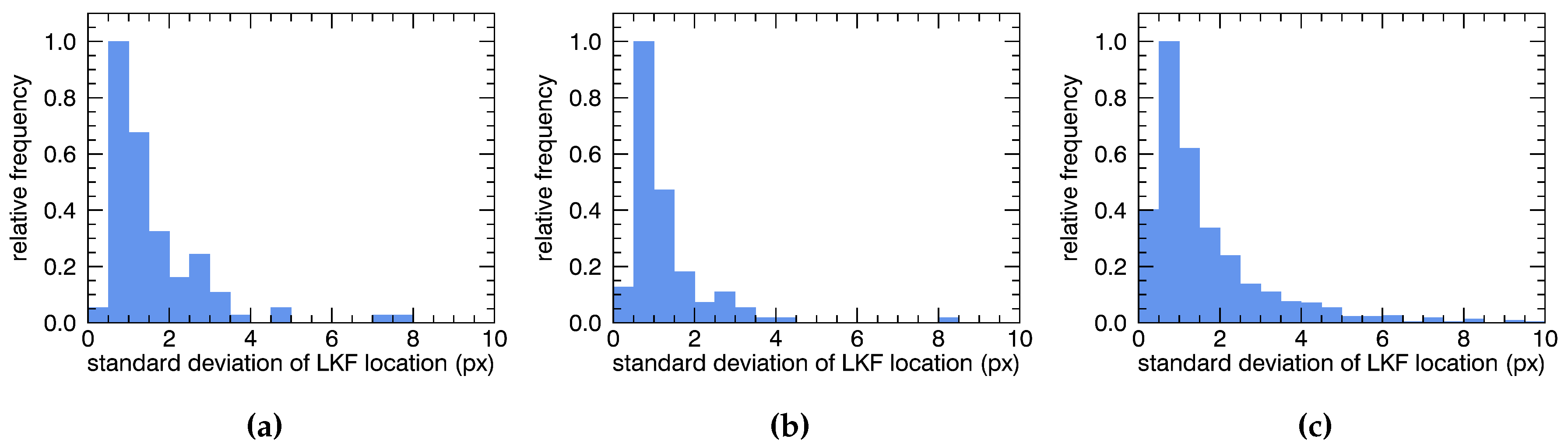
To evaluate the error in -direction, perpendicular to the linear feature, the vertices of the polylines are resampled to identical -coordinates (see Figure 8b). Once this is done, the standard deviation in -direction is calculated. This value quantifies the localization error of the LKF perpendicular to the line extension. The normalized error distribution functions are very similar for all evaluated cases and show consistent maxima at 0.75 px (9.4 km) (Figure 11).
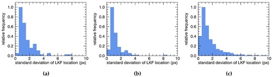
Figure 11.
Distribution of localization errors. (a) : N=129, = 0.75 px; (b) : N = 136, = 0.75 px; (c) : N = 1411, = 0.75 px.
The validation conducted using the visually determined reference data leads to the following conclusions. First, the intrinsic localization uncertainty of the reference data is 0.75 px and hence on the order of the spatial resolution of the dataset. The object detection results are equally well-localized. Second, there is an 8% uncertainty in line length inherent in the visual validation. Since all our error assessment is based on the comparison with the visually detected lines, the 8% length uncertainty must be regarded as the lower limit of the line length error. We find that the respective object detection error is of similar magnitude (8–12%). Overall, there is a very good agreement between the reference data and the results of the automated object detection.
3.2. Plausibility Testing
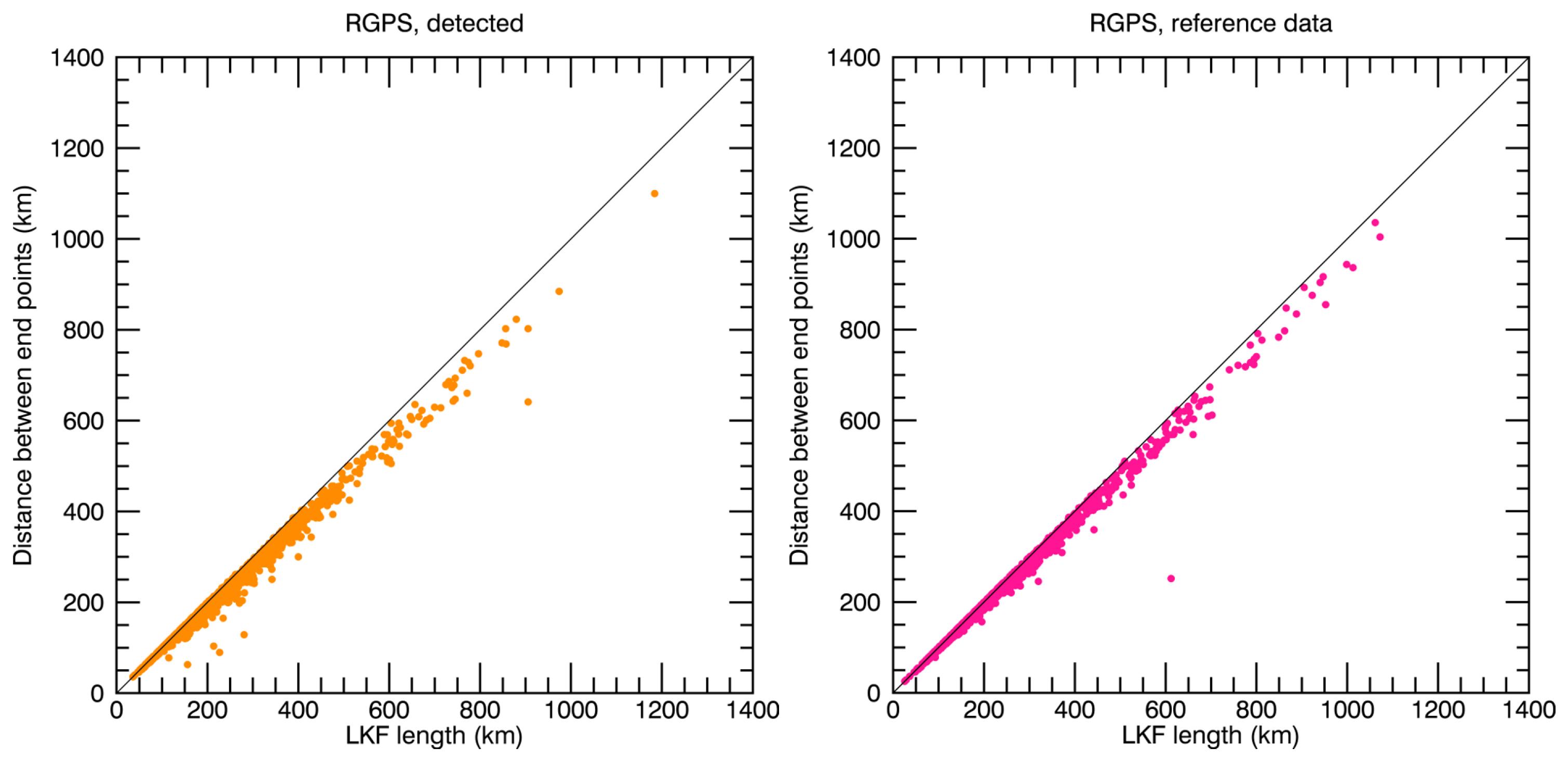
A simple benchmark for checking whether the detected objects are LKFs is to look at their curvature. An indicator of their curvature is the relation between the distance between end points and the integrated feature length along all individual vertices. If both values are plotted, they should approach the 1:1 line to indicate linearity. The results in Figure 12 show excellent agreement between integrated line length and endpoint distance in both the reference data and the results of the object detection.
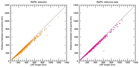
Figure 12.
Endpoint distance vs. integrated line length as an indicator of feature linearity. (a) Detected objects; (b) Reference data ().
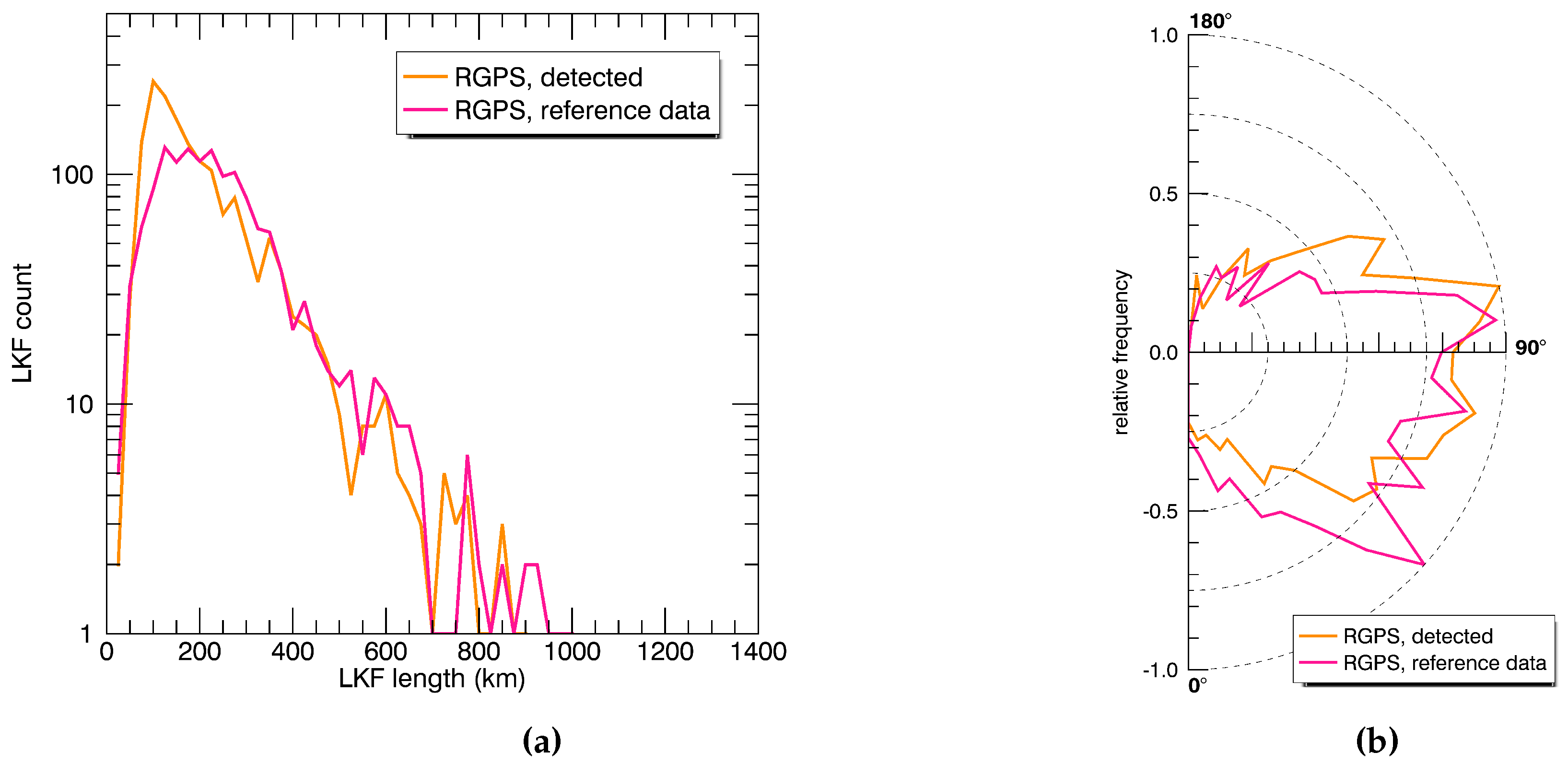
A lower limit of =7 px (87.5 km) was chosen which corresponds to the minimum size required for a human observer to unambiguously detect an LKF. The result of this test revealed that approximately 17% more objects were detected with the automated method than with the reference data. Still, the reference distribution of length scales is very well reproduced by the results of the object detection (Figure 13a).
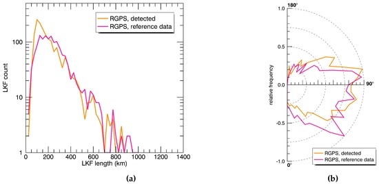
Figure 13.
Feature length and orientation. Lines having angles of 0° are oriented along the parallels, lines with 90° angles are oriented in meridional direction. (a) Feature length distribution; (b) Distribution of feature orientation angles.
Figure 13b shows the distribution of feature orientations of the detected and reference LKF. Orientation angles are given relative to the North direction and were computed for the line connecting start and endpoint of the LKF. To facilitate the visual interpretation, the data sets were normalized to compensate for the difference in absolute sample numbers. It can be seen that the features found by the object detection method are oriented along the same directions as the reference data, even though there is a more pronounced peak in the reference data at 45° orientation angle. In summary, the detected features fulfill the criterion of linearity stated in Section 2.3, and their length distribution and orientation are in line with the reference data.
From the results of this plausibility test and the validation conducted in Section 3.1, it can be concluded that the automatically detected objects can be regarded as representative for the LKF found visually in the original data set. Hence, it is possible to derive spatial statistics from LKF objects detected with the automated method.
4. Discussion
Several studies (e.g., [6,7,8,9,10],) analyze sea ice deformation features using pixel-based image segmentation. With such a pixel-based approach, the ability to interpret the spatial context of the deformation features is very limited. More versatile information on sea ice deformation features can be gained by extending the segmentation by an object detection step, which is able to identify and differentiate individual features. Only one recent study [34] exists which analyses sea ice deformation based on vectorized objects, but the authors focus on aspects of ice deformation retrieval that are different from our objectives, and their method is not directly applicable to our case. An older study [11,12] focused on the radar intensity variations in an image and implemented a method to divide bright linear structures in SAR images, which are most probably caused by ridges, into segments. They skeletonized the detected ridge structures to a width of one pixel and searched for intersections and end points, which represent “nodes” between individual segments. For further analyses, they used the single elements. We improved and extended this method. A ridge, or more general, a LKF may consist of more than one segment. In some cases, segments interrupted by small gaps have to be re-connected for, e.g., calculating statistics of length and orientation.
In our study we developed a validation scheme, which enables us to quantify both the errors in the reference data and the differences between the results of automated LKF extraction and the reference. The results of the proposed method are more flexible to use than those from approaches based on image segmentation and pixel-based retrievals, and allow a large variety of further analysis steps. We regard object detection as an advanced tool for sea ice deformation analysis and highlight some of the possible applications of our approach with the following examples.
Since with our method detected LKF can be traced individually, this offers several advantages:
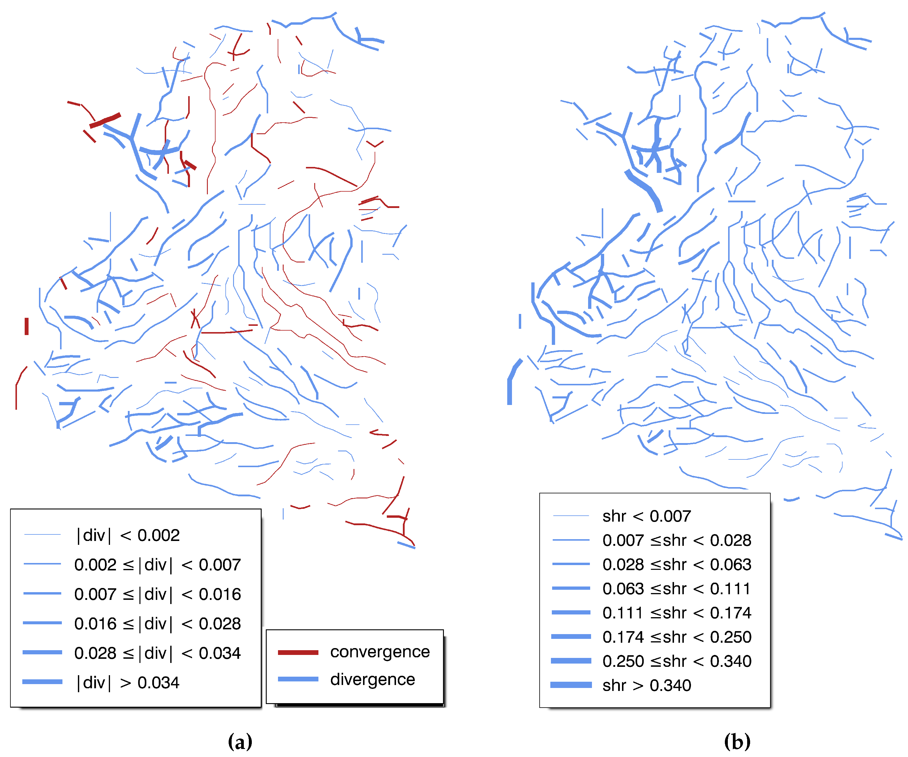
- analysis of individual features: as the geographical coordinates of each vertex of each detected object are known, LKFs can be analyzed on an individual basis. Values from the original deformation images or other parameters can be easily mapped back onto the observed features (Example: divergence and shear maps for the entire spatial domain, Figure 14).
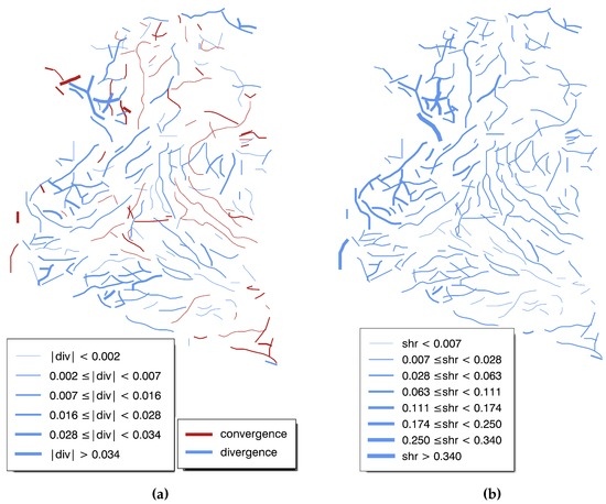 Figure 14. Subsets/mapping of gridded image data. (a) Divergence (1/day); (b) Shear (1/day).
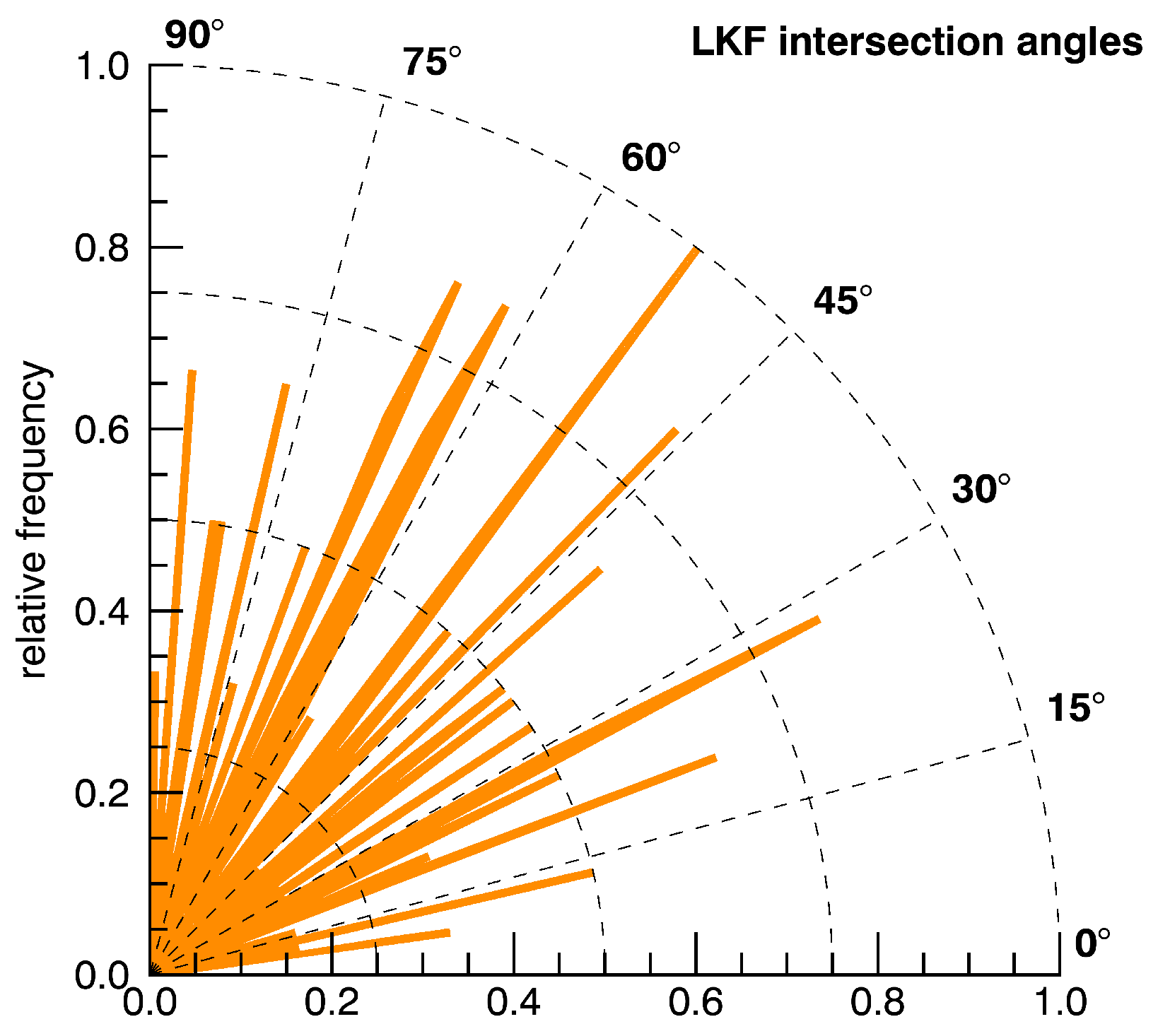
 - LKF intersection angles: fracture mechanics of the ice cause “typical” fracture patterns, and the intersection angles depend on properties of the material, similar to stress faulting in rocks. Here, we also consider cases in which one LKF ends in the vicinity of another LKF instead of intersecting it by applying a simple distance criterion. Each pair of LKFs (consiting of several segments with slightly varying orientations) is approximated by a pair of lines fixed to the respective start- and endpoints, and the intersection angle between those lines is calculated. The result for the entire scene from Figure 6a is shown in Figure 15. The relationship between fracture angles and strain magnitude is rather complex and depends on the type of strain (e.g., shear or divergence) and on material properties [1]. With given strain rates (such as in Figure 14) and LKF intersection angles derived from the detected objects, the data basis is available to analyze the material/fracturing properties of the sea ice in more detail. However, this type of analysis would exceed the scope of this study.
 Figure 15. LKF intersection angles (bin size = 1°).
An extension of the object detection method towards time series analysis is relatively easy. Possible applications here include an evaluation of feature recurrence/persistence by tracking of individual features over the time series (persistance) and the analysis of feature occurrence frequency at fixed locations (recurrence). Since our method allows tracking of individual LKF objects, the type of time series analysis conducted by [9] could be extended and refined to obtain a clearer picture of LKF evolution.
Since our object detection method is designed to work independently of input data type, it can be directly used to analyze the output of sea ice model simulations, as well. By resolving individual LKFs, our vector-based approach thus allows a significantly higher level of detail in the validation of the fracture mechanics implemented in sea ice models. It is able to extend the work by e.g., [3,20,35,36], and can help to improve the representation of sea ice rheology in climate models.
5. Conclusions
A method for an automated LKF detection which generates results at a high level of accuracy is demonstrated in the present study. On the basis of sea ice deformation images, we extend the widely-used pixel-based segmentation approach by adding an additional vectorization step. We explicitly allow LKFs to intersect and develop a basic semantic ruleset to recognize individual segments in an LKF. Our method is validated using visually identified LKFs as reference data. Excellent agreement is found between the reference LKFs and the results of the automated feature detection for the entire set of examined images. The number of objects used for the comparison is sufficiently high to generalize the results of our analysis. The detected objects have a location accurracy of 0.75 px and an uncertainty in line length of 12%. Because the detected linear features are object-based, it is straightforward to analyse their spatial context. For this purpose, properties such as number, linearity, orientation, length, and the angles of intersecting features are evaluated. Subsets of the detected features can be easily generated, based for instance on their geographic location, but many more possibilities exist. This paper introduces a versatile tool for an advanced geospatial analysis of linear features in sea ice, which can be, for instance, helpful for validating sea ice rheology in ice-ocean models or to study material/fracturing behaviour of sea ice.
Author Contributions
Stefanie Linow designed and implemented the method. Both authors together discussed details of the method, implementation and validation, and prepared the text.
Conflicts of Interest
The authors declare no conflict of interest.
Appendix A
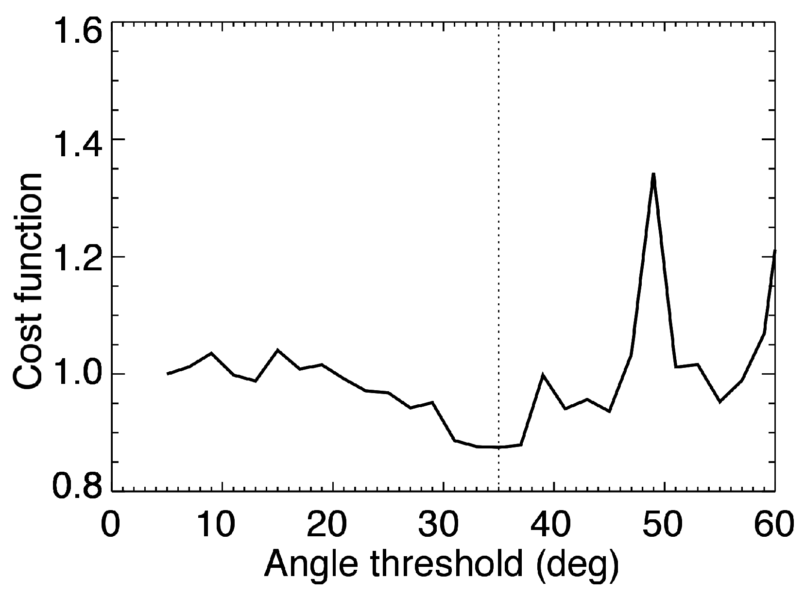
We can estimate a suitable value for the intersection angle threshold by evaluating two parameters on the basis of the data set. The first one is the linearity of the detected features (see Figure 12a). With an increasing angle tolerance, the linearity of the detected features will decrease, as more false matches are included in the data set. The linearity can be expressed in terms of the ratio between the integrated line length and the endpoint distance, .
The second parameter to evaluate is the error in line lenght between reference and detected lines. This value indicates how well the detected lines can be matched to the reference data. It decreases with increasing angular tolerance as more suitable objects are found. This parameter is derived from Figure 8a and Figure 9a, and denoted by . The subscript n indicates that the values were normalized to the interval in order to give equal weight to both parameters. Based on those considerations, we minimize the following cost function F: . The results for a range of intersection angle thresholds is shown in Figure A1. The minimum of F can be found at 35°, and this value has been subsequently used as an upper threshold for the intersection angle.

Figure A1.
Cost function for intersection angle tolerance values ranging from 5° to 60°, in steps of 2°. The dotted line marks the 35° threshold.
Figure A1.
Cost function for intersection angle tolerance values ranging from 5° to 60°, in steps of 2°. The dotted line marks the 35° threshold.
References
- Erlingsson, B. Two-dimensional deformation patterns in sea ice. J. Glaciol. 1988, 34, 301–308. [Google Scholar] [CrossRef]
- Schulson, E.M. Compressive shear faults within arctic sea ice: Fracture on scales large and small. J. Geophys. Res. 2004, 109, C07016. [Google Scholar] [CrossRef]
- Rampal, P.; Bouillon, S.; Ólason, E.; Morlighem, M. neXtSIM: A new Lagrangian sea ice model. Cryosphere 2016, 10, 1055–1073. [Google Scholar] [CrossRef]
- Marsan, D.; Stern, H.; Lindsay, R.; Weiss, J. Scale Dependence and Localization of the Deformation of Arctic Sea Ice. Phys. Rev. Lett. 2004, 93, 178501. [Google Scholar] [CrossRef] [PubMed]
- Hutchings, J.; Heil, P.; Steer, A.; Hibler, W. Subsynoptic scale spatial variability of sea ice deformation in the western Weddell Sea during early summer. J. Geophys. Res. 2012, 117, C01002. [Google Scholar] [CrossRef]
- Onana, V.D.P.; Kurtz, N.T.; Farrell, S.L.; Koenig, L.S.; Studinger, M.; Harbeck, J.P. A Sea-Ice Lead Detection Algorithm for Use With High-Resolution Airborne Visible Imagery. IEEE Trans. Geosci. Remote Sens. 2013, 51, 38–56. [Google Scholar] [CrossRef]
- Willmes, S.; Heinemann, G. Pan-Arctic lead detection from MODIS thermal infrared imagery. Ann. Glaciol. 2015, 56, 29–37. [Google Scholar] [CrossRef]
- Lindsay, R.W.; Rothrock, D.A. Arctic sea ice leads from advanced very high resolution radiometer images. J. Geophys. Res. 1995, 100, 4533–4544. [Google Scholar] [CrossRef]
- Bröhan, D.; Kaleschke, L. A Nine-Year Climatology of Arctic Sea Ice Lead Orientation and Frequency from AMSR-E. Remote Sens. 2014, 6, 1451–1475. [Google Scholar] [CrossRef]
- Miles, M.; Barry, R. A 5-year satellite climatology of winter sea ice leads in the western Arctic. J. Geophys. Res. 1998, 103, 21723–21734. [Google Scholar] [CrossRef]
- Vesecky, J.F.; Smith, M.P.; Samadani, R. Extraction of Lead and Ridge Characteristics from SAR Images of Sea Ice. IEEE Trans. Geosci. Remote Sens. 1990, 28, 740–744. [Google Scholar] [CrossRef]
- Vesecky, J.F.; Smith, M.P.; Samadani, R. Remote Sensing of Pressure Ridge and Lead Characteristics Using Sar Images of Sea Ice. In Proceedings of the 10th Annual International Geoscience and Remote Sensing Symposium, College Park, MD, USA, 20–24 May 1990; pp. 1871–1874. [Google Scholar]
- Dierking, W.; Dall, J. Sea Ice Deformation State From Synthetic Aperture Radar Imagery—Part I: Comparison of C- and L-Band and Different Polarization. IEEE Trans. Geosci. Remote Sens. 2007, 45, 3610–3622. [Google Scholar] [CrossRef]
- Kwok, R.; Curlander, J.; McConnell, R.; Pang, S. An Ice Motion Tracking System at the Alaska SAR Facility. IEEE J. Ocean. Eng. 1990, 15, 44–54. [Google Scholar] [CrossRef]
- Lindsay, R.; Zhang, J.; Rothrock, D. Sea Ice Deformation Rates From Satellite Measurements and in a Model. Atmos. Ocean 2003, 41, 35–47. [Google Scholar] [CrossRef]
- Kwok, R. Declassified high-resolution visible imagery for Arctic sea ice investigations: An overview. Remote Sens. Environ. 2014, 142, 44–56. [Google Scholar] [CrossRef]
- Thorndike, A.; Colony, R. Sea ice motion in response to geostrophic winds. J. Geophys. Res. 1982, 87, 5845–5852. [Google Scholar] [CrossRef]
- Bouillon, S.; Rampal, P. On producing sea ice deformation data sets from SAR-derived sea ice motion. Cryosphere 2015, 9, 663–673. [Google Scholar] [CrossRef]
- Weiss, J. Drift, Deformation and Fracture of Sea Ice. A Perspective Across Scales; Springer Netherlands: Dordrecht, The Netherlands, 2013. [Google Scholar]
- Girard, L.; Weiss, J.; Molines, J.M.; Barnier, B.; Bouillon, S. Evaluation of high-resolution sea ice models on the basis of statistical and scaling properties of Arctic sea ice drift and deformation. J. Geophys. Res. 2009, 114, 281–325. [Google Scholar] [CrossRef]
- Canny, J. A computational approach to edge detection. IEEE Trans. Pattern Anal. Machine Intell. 1986, 8, 679–698. [Google Scholar] [CrossRef]
- Marr, D.; Hildreth, E. Theory of Edge Detection. Proc. R. Soc. Lond. B 1980, 207, 187–217. [Google Scholar] [CrossRef] [PubMed]
- Lindeberg, T. Principles for Automatic Scale Selection. In Handbook on Computer Vision and Applications; Academic Press: Boston, MA, USA, 1999; Volume 2, pp. 239–274. [Google Scholar]
- Arbelaez, P.; Maire, M.; Fowlkes, C.; Malik, J. Contour detection and hierarchical image segmentation. IEEE Trans. Pattern Anal. Mach. Intell. 2010, 33, 898–916. [Google Scholar] [CrossRef] [PubMed]
- Szeliski, R. Computer Vision—Algorithms and Applications; Texts in Computer Science; Springer: London, UK, 2011. [Google Scholar]
- Gonzalez, R.C.; Woods, R.E. Digital Image Processing, 3rd ed.; Prentice-Hall, Inc.: Upper Saddle River, NJ, USA, 2006. [Google Scholar]
- Steger, C. An Unbiased Detector of Curvilinear Structures. IEEE Trans. Pattern Anal. Mach. Intell. 1998, 20, 113–125. [Google Scholar] [CrossRef]
- Zhou, J.; Bischof, W.; Caelli, T. Road tracking in aerial images based on human-computer interaction and Bayesian filtering. ISPRS J. Photogramm. Remote Sens. 2006, 61, 108–124. [Google Scholar] [CrossRef]
- Poullis, C.; You, S. Delineation and geometric modeling of road networks. ISPRS J. Photogramm. Remote Sens. 2010, 65, 165–181. [Google Scholar] [CrossRef]
- Maire, M.; Arbeláez, P.; Fowlkes, C.; Malik, J. Using contours to detect and localize junctions in natural images. In Proceedings of the Conference on Computer Vision and Pattern Recognition, Anchorage, AK, USA, 23–28 June 2008; pp. 1–8. [Google Scholar]
- Press, W.H.; Teukolsky, S.A.; Vetterling, W.T.; Flannery, B.P. Numerical Recipes 3rd Edition: The Art of Scientific Computing; Cambridge University Press: New York, NY, USA, 2007. [Google Scholar]
- Martin, S. Polynyas. In Encyclopedia of Ocean Sciences; John, H., Steele, E., Eds.; Academic Press: Oxford, UK, 2001; pp. 2241–2247. [Google Scholar]
- Martin, D.; Fowlkes, C.; Malik, J. Learning to detect natural image boundaries using local brightness, color, and texture cues. IEEE Trans. Pattern Anal. Mach. Intell. 2004, 26, 530–549. [Google Scholar] [CrossRef] [PubMed]
- Miao, X.; Xie, H.; Ackley, S.F.; Zheng, S. Object-based Arctic sea ice ridge detection from high-spatial-resolution imagery. IEEE Geosci. Remote Sens. Lett. 2016, 13, 787–791. [Google Scholar] [CrossRef]
- Kwok, R.; Hunke, E.C.; Maslowski, W.; Menemenlis, D.; Zhang, J. Variability of sea ice simulations assessed with RGPS kinematics. J. Geophys. Res. 2008, 113, C11012. [Google Scholar] [CrossRef]
- Kwok, R. Sea ice convergence along the Arctic coasts of Greenland and the Canadian Arctic Archipelago: Variability and extremes (1992–2014). Geophys. Res. Lett. 2015, 42, 7598–7605. [Google Scholar] [CrossRef]


© 2017 by the authors. Licensee MDPI, Basel, Switzerland. This article is an open access article distributed under the terms and conditions of the Creative Commons Attribution (CC BY) license (http://creativecommons.org/licenses/by/4.0/).