
Estimation and Analysis of Spatiotemporal Dynamics of the Net Primary Productivity Integrating Efficiency Model with Process Model in Karst Area

Abstract
:
1. Introduction
2. Study Area and Materials
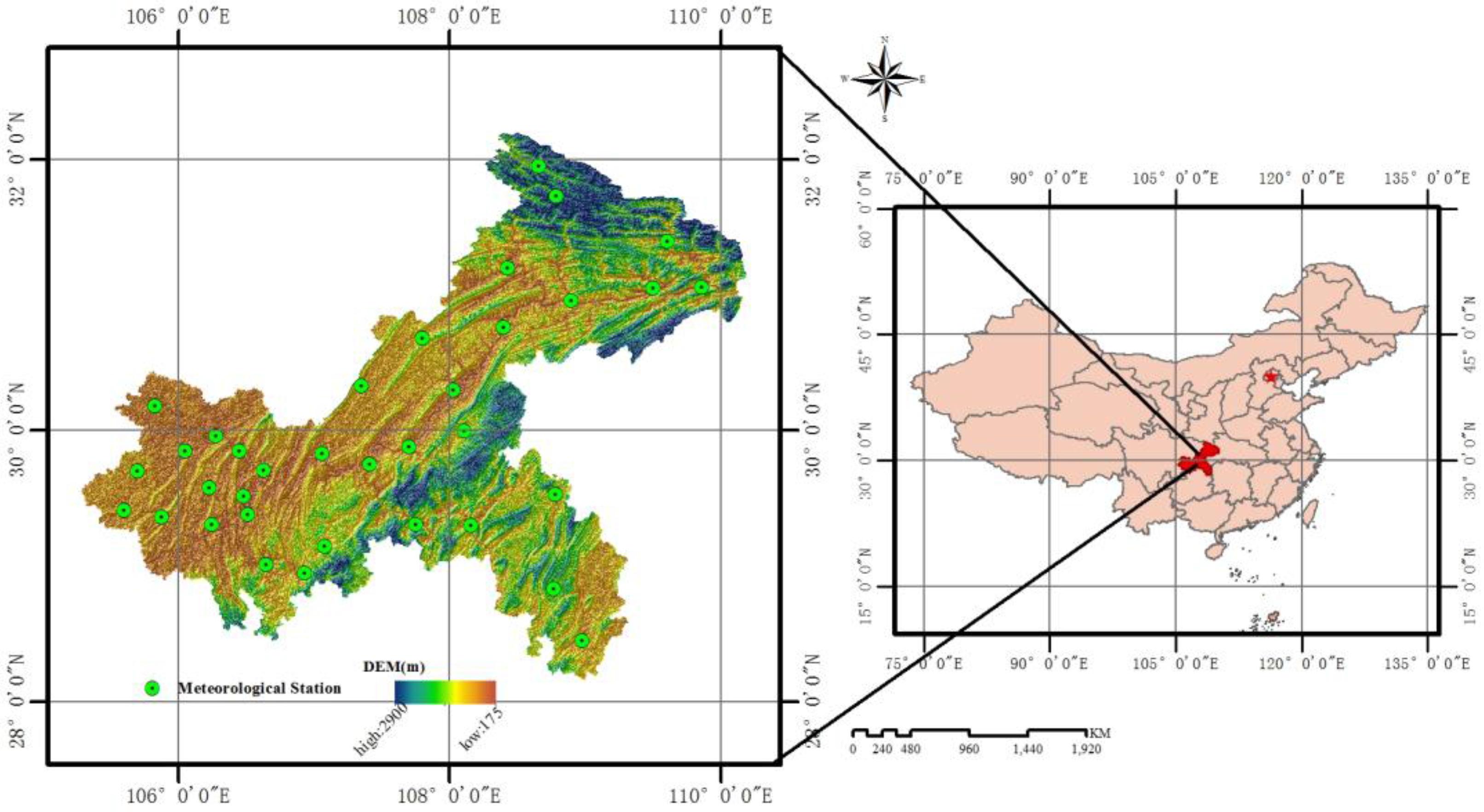
2.1. Study Area
2.2. Data Used in This Study
2.2.1. Remote Sensing Data
2.2.2. Meteorological Data
2.2.3. Model Parameter Data
2.2.4. Validation and Comparison of the Derived NPP
3. Methodology
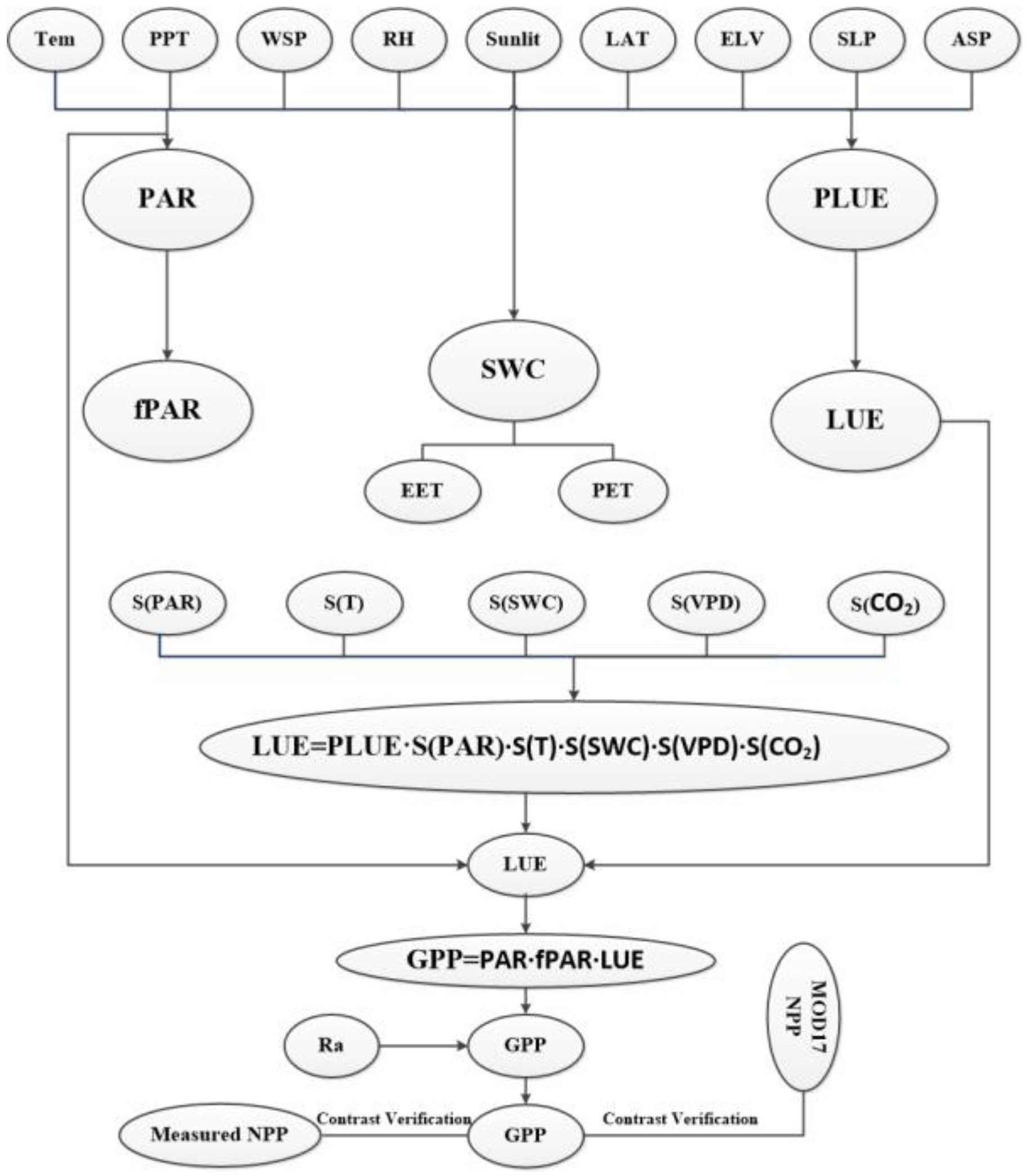
3.1. GLOPEM Model
3.2. CEVSA Model
3.3. Developing GLOPEM Model and CEVSA Model : GLOPEM-CEVSA Model
4. Results
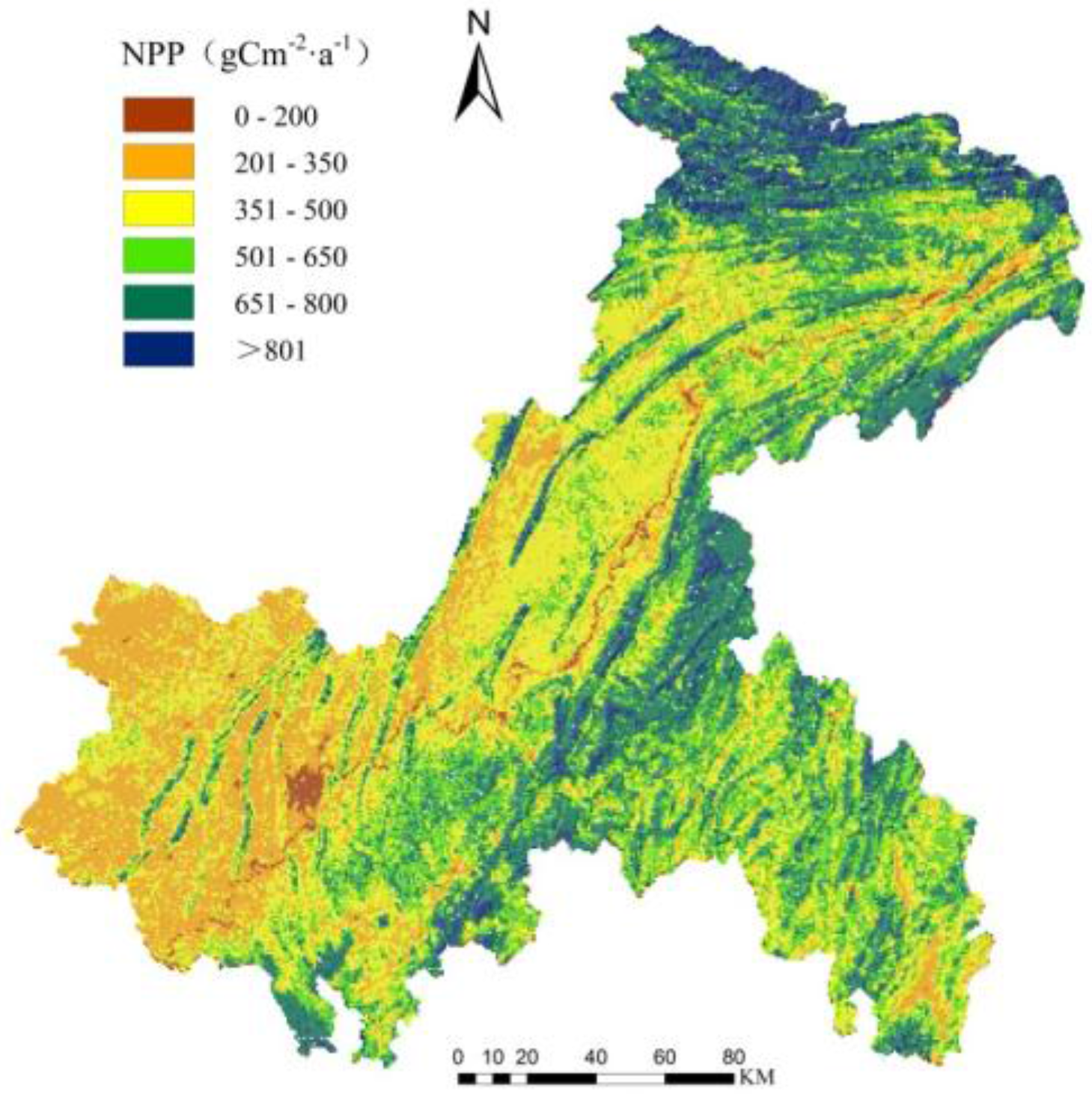
4.1. NPP Spatial Distribution and Change
4.2. The Distribution in Different Vegetation Types
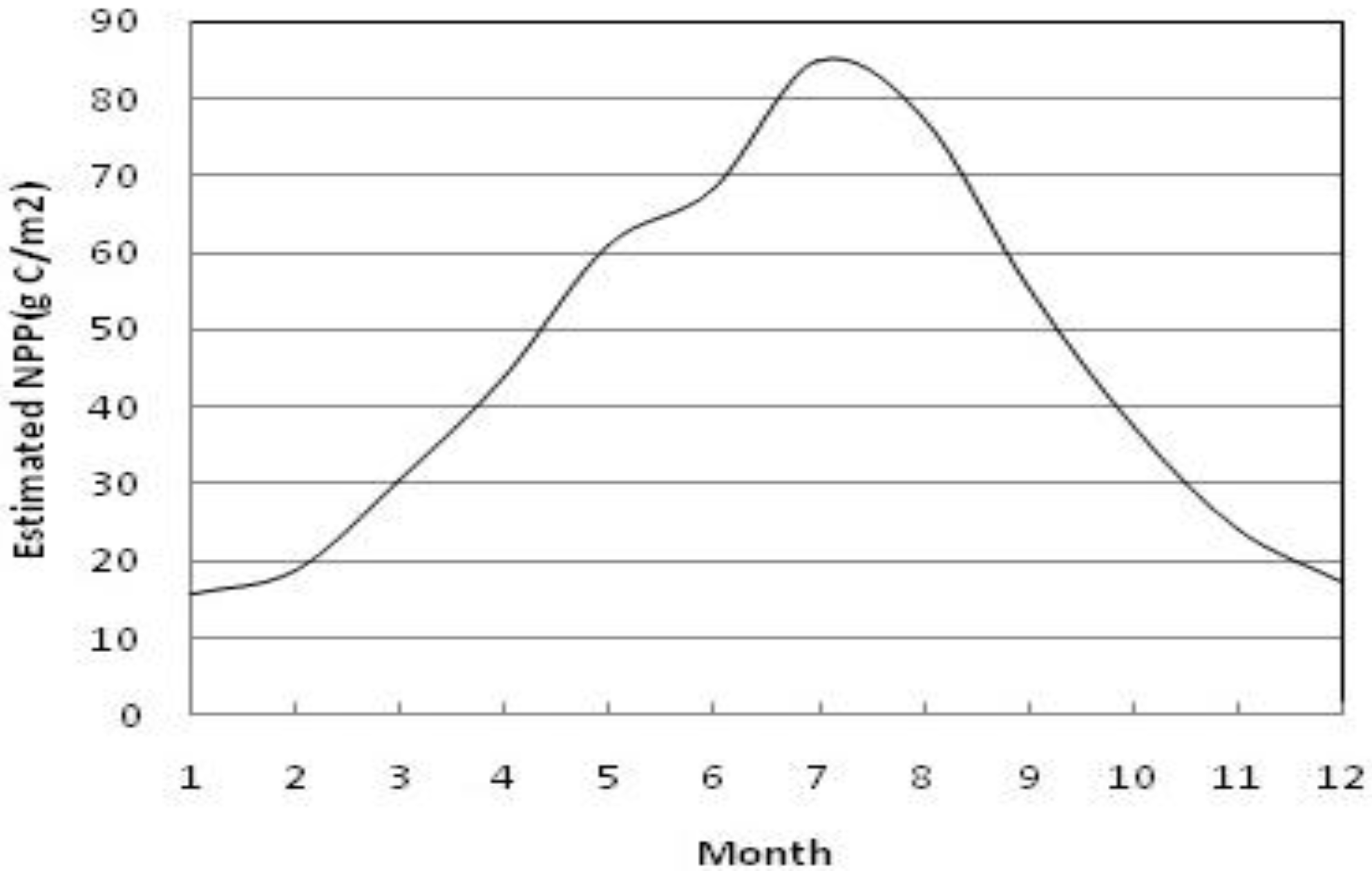
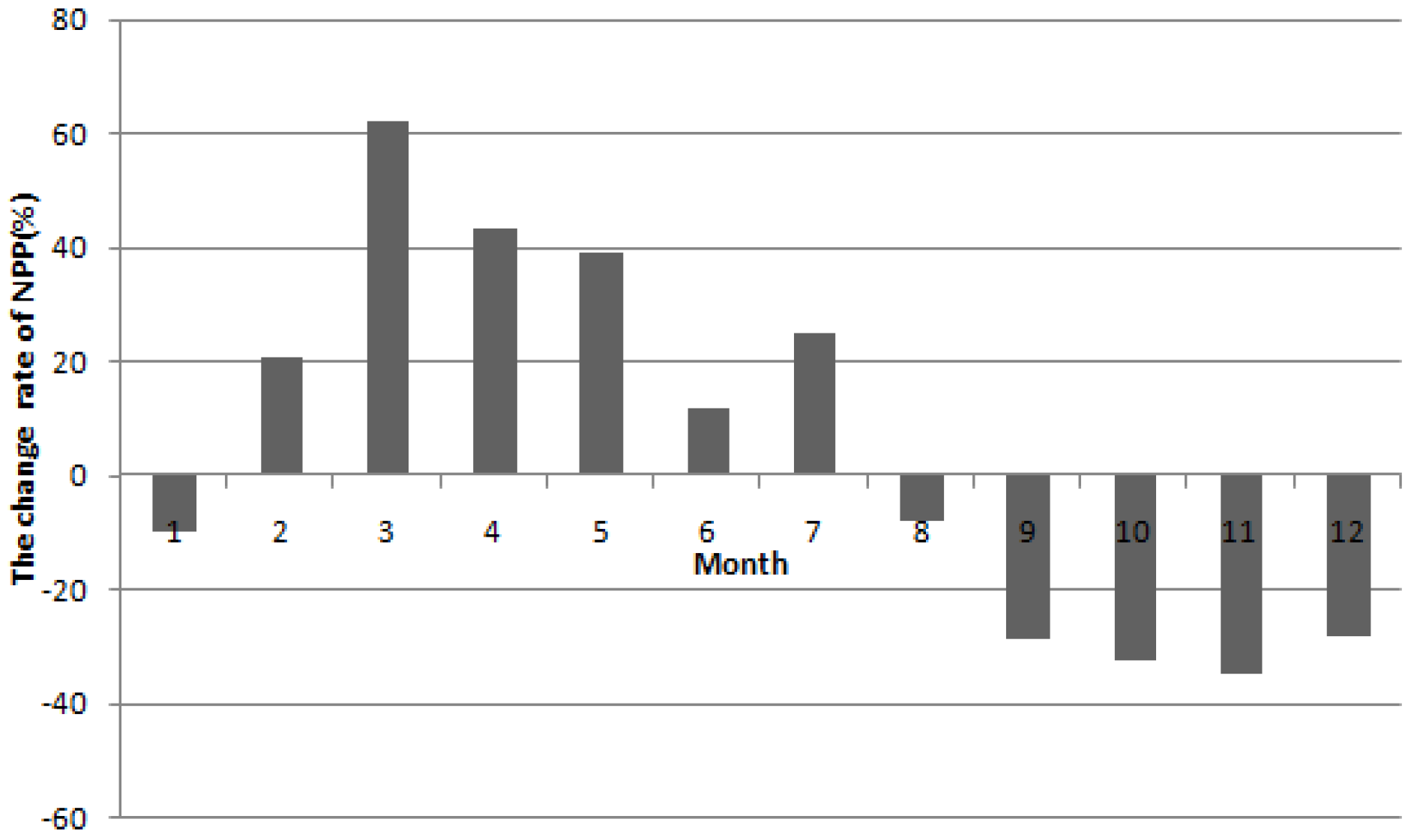
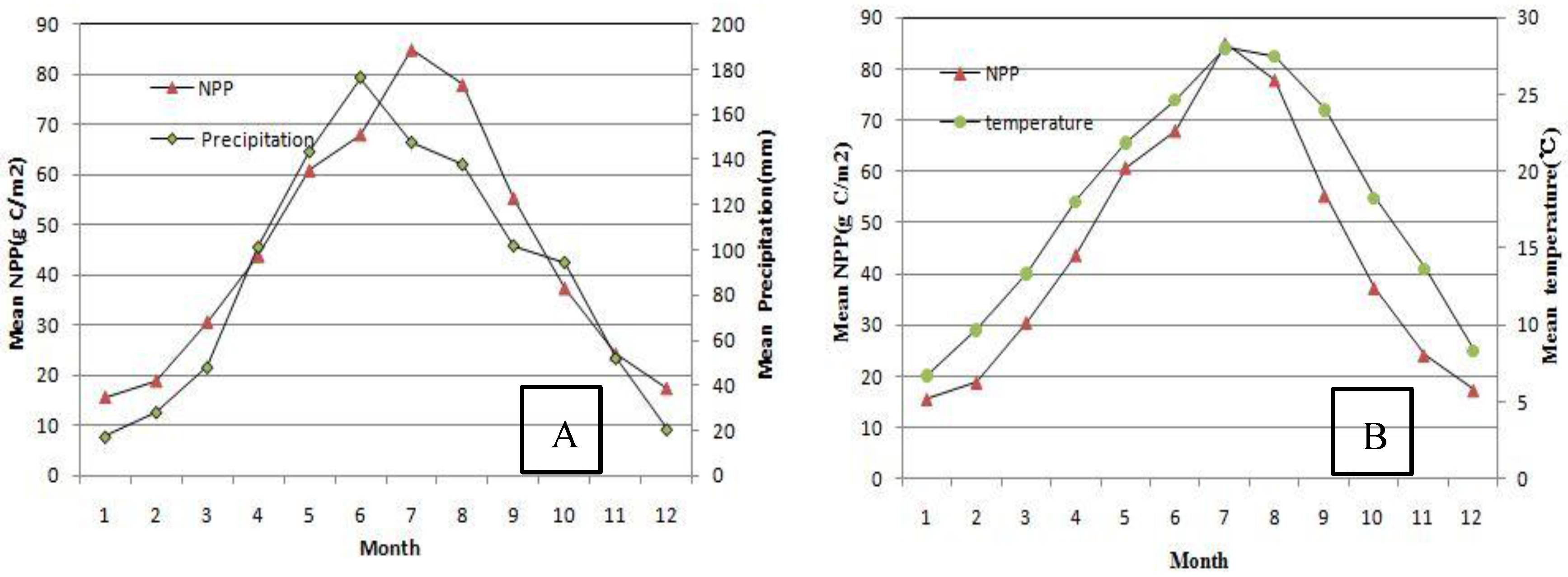
4.3. Monthly Variation of NPP Value
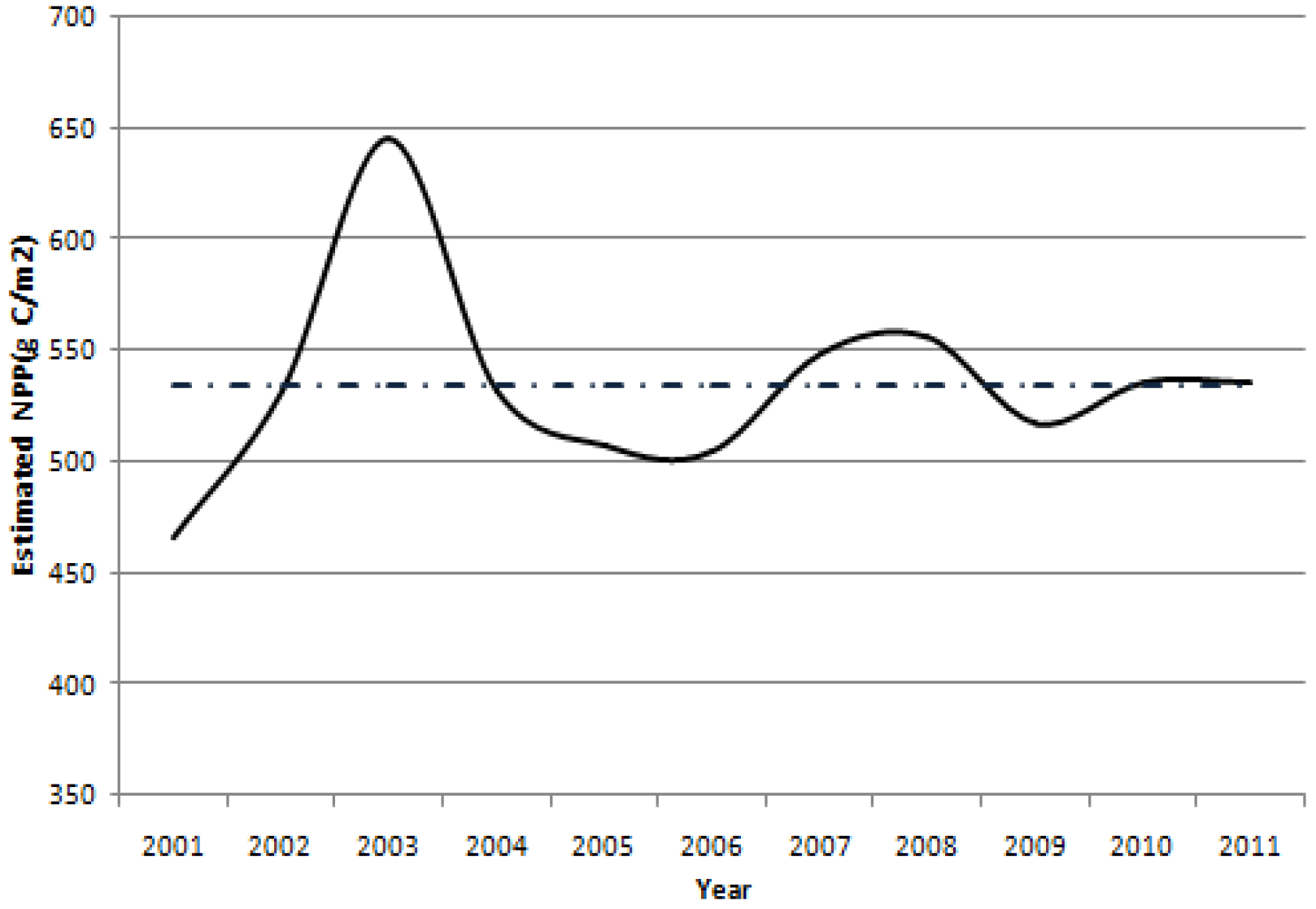
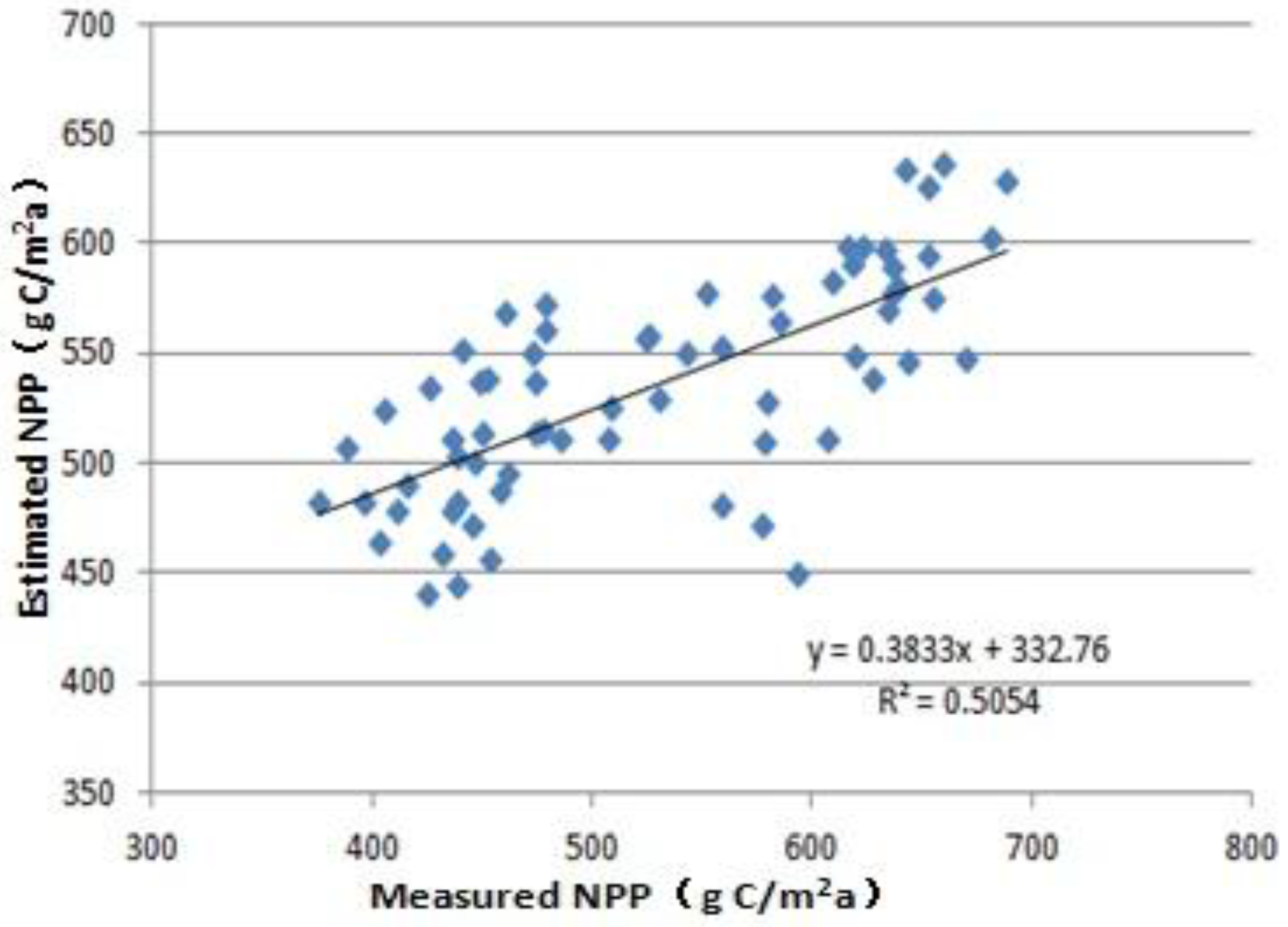
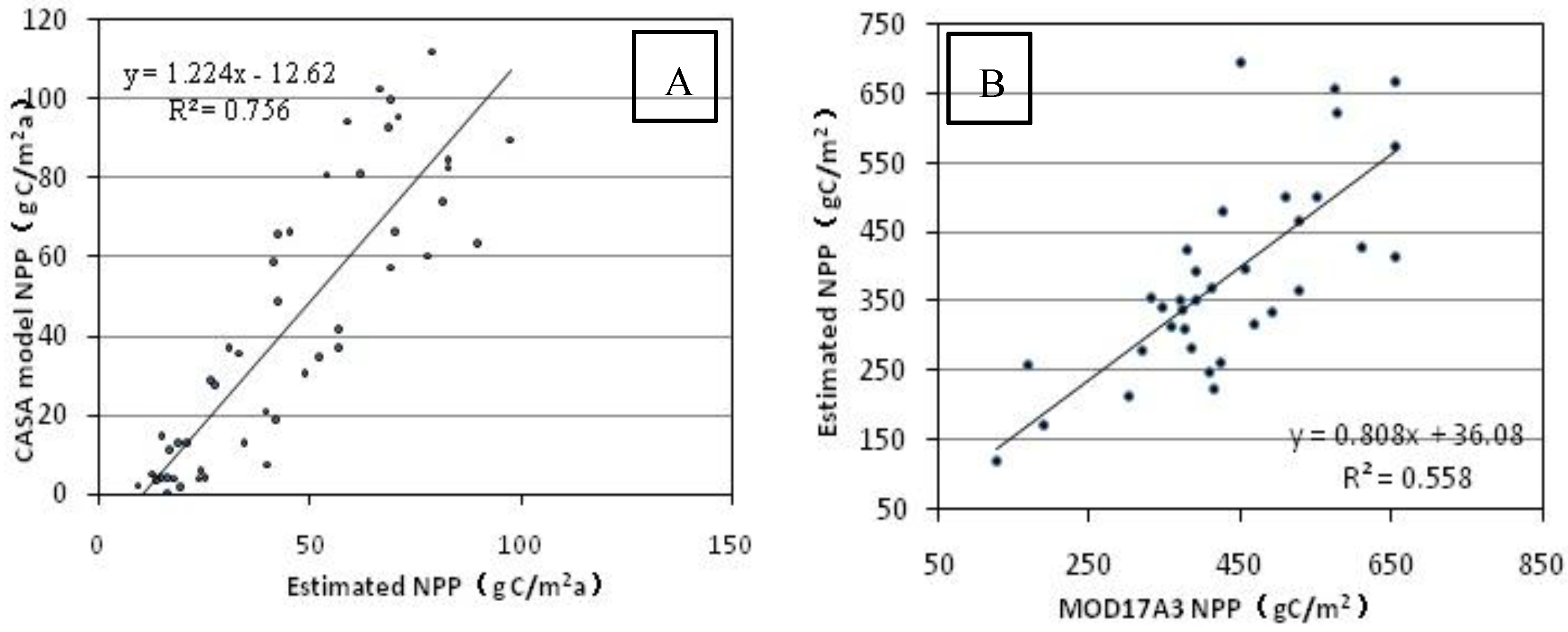
4.4. Spatial and Temporal Comparison among NPP Values
5. Discussion
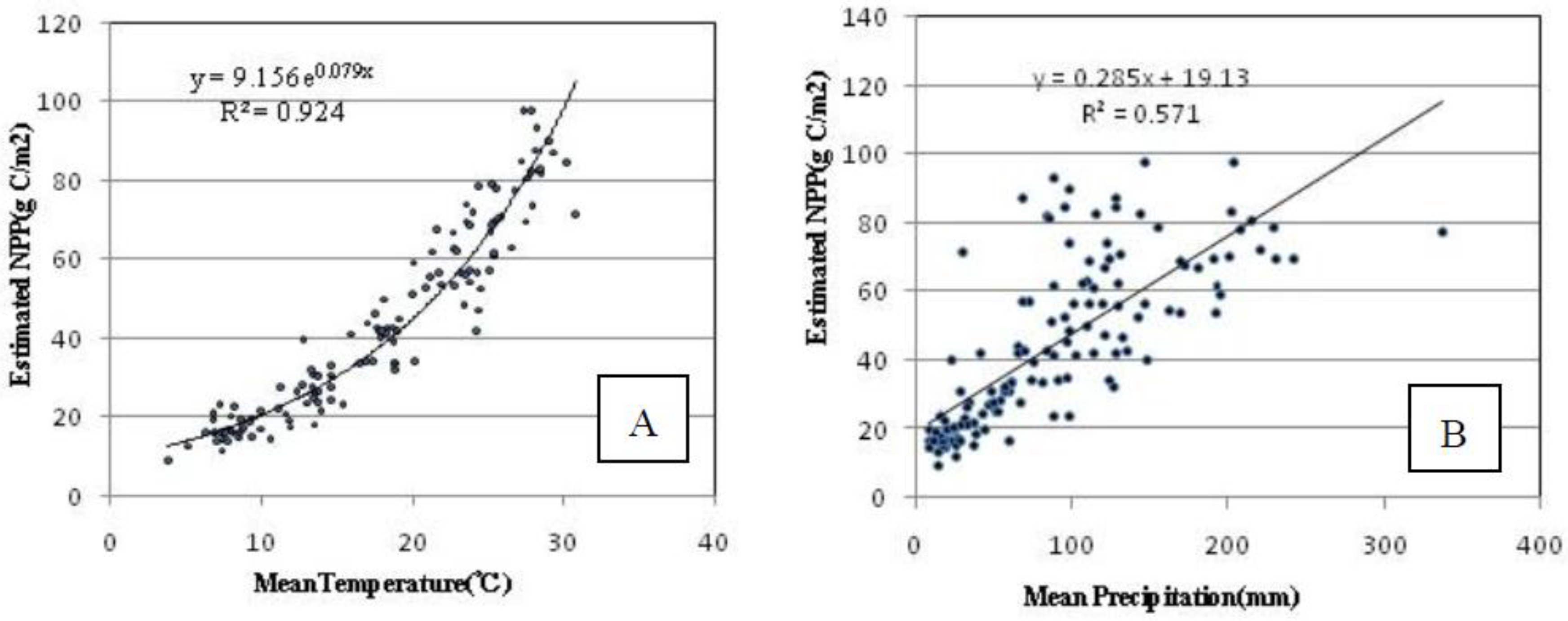
5.1. Relationships between NPP and Meteorological Factors
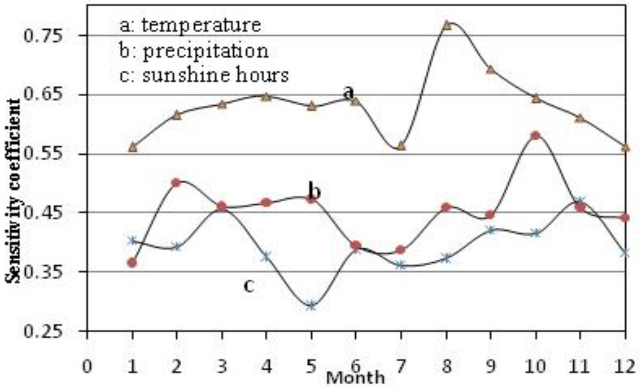
5.2. Sensitivity Analysis
5.3.Uncertainties of the Model and the Interference of Mixed Pixels
6. Conclusions
Acknowledgments
Author Contributions
Conflicts of Interest
References
- Piao, S.; Fang, J.; He, J. Variations in vegetation net primary production in the Qinghai-Xizang Plateau, China, from 1982 to 1999. Clim. Chang. 2006, 74, 253–267. [Google Scholar] [CrossRef]
- Lobell, D.B.; Hicke, J.A.; Asner, G.P. Satellite estimates of productivity and light use efficiency in United States agriculture 1982–1998. Glob. Chang. Biol. 2002, 8, 722–735. [Google Scholar] [CrossRef]
- Field, C.B.; Randerson, J.T.; Malmström, C.M. Global net primary production: Combining ecology and remote sensing. Remote Sens. Environ. 1995, 51, 74–88. [Google Scholar] [CrossRef]
- Nemani, R.R.; Charles, D.; Hashimoto, K.H. Climate-driven increases in global terrestrial net primary production from 1982 to 1999. Science 2003, 300, 1560–1563. [Google Scholar] [CrossRef] [PubMed]
- Yu, G.R.; Wen, X.F.; Li, Q.K.; Zhang, L.; Ren, C.Y.; Liu, Y.F.; Guan, D.X. Seasonal patterns and environmental control of ecosystem respiration in subtropical and temperature forests in China. Sci. China Ser. D 2005, 48, 93–105. [Google Scholar] [CrossRef]
- Mu, S.J.; Chen, Y.Z.; Li, J.L.; Ju, W.M.; Odeh, I.O.A.; Zou, X.L. Grassland dynamics in response to climate change and human activities in Inner Mongolia, China between 1985 and 2009. Rangel. J. 2013, 35, 315–329. [Google Scholar] [CrossRef]
- Turner, D.P.; Ollinger, S.V.; Kimball, J.S. Integrating remote sensing and ecosystem process models for landscape-to regional-scale analysis of the carbon cycle. Bioscience 2004, 54, 573–584. [Google Scholar] [CrossRef]
- Cao, M.; Prince, S.; Tao, B.; Small, J.; Li, K. Regional pattern and interannual variations in global terrestrial carbon uptake in response to changes in climate and atmospheric CO2. Tellus B 2005, 57, 210–217. [Google Scholar] [CrossRef]
- Rayner, P.J.; Scholze, M.; Knorr, W.; Kaminski, T.; Giering, R.; Widmann, H. Two decades of terrestrial carbon fluxes from a carbon cycle data assimilation system. Glob. Biogeochem. Cycles 2005, 19, 202–214. [Google Scholar] [CrossRef]
- Li, X.; Zhu, Z.; Zeng, H.; Piao, S. Estimation of gross primary production in China (1982–2010) with multiple ecosystem models. Ecol. Model. 2016, 324, 33–44. [Google Scholar] [CrossRef]
- Woodward, F.I.; Smith, M.T.; Emanuel, W.R. A global land primary productivity and phytogeography model. Glob. Biogeochem. Cycles 1995, 9, 471–490. [Google Scholar] [CrossRef]
- Chen, J.; Yan, H.; Wang, S.; Guo, Y.; Huang, M.; Wang, J.; Xiao, X. Estimation of gross primary productivity in Chinese terrestrial ecosystems by using VPM model. Quat. Sci. 2014, 34, 732–742. [Google Scholar] [CrossRef]
- Chen, L.; Liu, G.; Li, H. Estimating net primary productivity of terrestrial vegetation in China using remote sensing. J. Remote Sens. 2002, 2, 129–135. (In Chinese) [Google Scholar]
- Potter, C.S.; Randerson, J.T.; Field, C.B.; Matson, P.A.; Vitousek, P.M.; Mooney, H.A.; Klooster, S.A. Terrestrial ecosystem production: A process model based on global satellite and surface data. Glob. Biogeochem. Cycles 1993, 7, 811–841. [Google Scholar] [CrossRef]
- Hazarikaa, M.K.; Yasuoka, Y.; Ito, A.; Dye, D. Estimation of net primary productivity by integrating remote sensing data with an ecosystem model. Remote Sens. Environ. 2005, 94, 298–310. [Google Scholar] [CrossRef]
- Prince, S.D.; Goward, S.N. Global primary production: A remote sensing approach. J. Biogeogr. 1995, 22, 815–835. [Google Scholar] [CrossRef]
- Running, S.; Ramakrishna, R.; Heinsch, F.; Zhao, M.; Reeves, M.; Hashimoto, H. A continuous satellite-derived measure of global terrestrial primary production. BioScience 2004, 54, 547–560. [Google Scholar] [CrossRef]
- Wang, J.B.; Liu, J.; Shao, Q.; Liu, R.; Fan, J.; Chen, Z. Spatial-temporal patterns of net primary productivity for 1988–2004 based on GLOPEM-CEVSA model in the “Three-river Headwaters ”region of Qinghai province, China. Chin. J. Plant Ecol. 2009, 33, 254–269. [Google Scholar]
- Yuan, J.; Niu, Z.; Wang, C.L. Vegetation NPP distribution based on MODIS data and CASA model—A case study of northern Hebei Province. Chin. Geogr. Sci. 2006, 16, 334–341. [Google Scholar] [CrossRef]
- Hutchinson, M.F.; Xu, T. Anusplin Version 4.4, Anuclim Version 6.1; Fenner School of Environment and Society, Australian National University: Canberra, Australia, 2004. [Google Scholar]
- Li, J.; Cui, Y.; Liu, J.; Shi, W.; Qin, Y. Estimation and analysis of net primary productivity by integrating MODIS remote sensing data with a light use efficiency model. Ecol. Model. 2016, 252, 3–10. [Google Scholar] [CrossRef]
- Prince, S.D. A model of regional primary production to use with coarse resolution satellite data. Int. J. Remote Sens. 1991, 12, 1313–1330. [Google Scholar] [CrossRef]
- Cao, M. K.; Prince, S.D.; Small, J.; Goetz, S.J. Remotely sensed interannual variations and trends in terrestrial net primary productivity 1981-2000. Ecosystems 2004, 7, 233–242. [Google Scholar] [CrossRef]
- Goetz, S.J.; Prince, S.P.; Small, J.; Gleason, A.C.R. Inter annual variability of global terrestrial primary production: Results of a model driven with global satellite observations. J. Geophys. Res. 2000, 105, 20077–20091. [Google Scholar] [CrossRef]
- Gu, F.; Cao, M.; Wen, X.; Liu, Y.; Tao, B. A comparison between simulated and measured CO2 and water flux in a subtropical coniferous forest. Sci. China Ser. D Earth Sci. 2006, 49 (Suppl. II), 241–251. [Google Scholar] [CrossRef]
- Van Laake, P.E.; Sanchez-Azofeifa, G.A. Simplified atmospheric radiative transfer modelling for estimating incident PAR using MODIS atmosphere products. Remote Sens. Environ. 2004, 1, 98–113. [Google Scholar] [CrossRef]
- Zhu, W.Q.; Pan, Y.Z.; Zhang, J.S. Estimation of net primary productivity of Chinese terrestrial vegetation based on remote sensing. Plant Ecol. 2007, 31, 413–424. [Google Scholar] [CrossRef]
- Zhao, G.; Wang, J.; Fan, W.; Ying, T. Vegetation net primary productivity in Northeast China in 2000–2008: Simulation and seasonal change. Chin. J. Appl. Ecol. 2011, 22, 621–630. (In Chinese) [Google Scholar]
- Collatz, G.; Ball, J.; Grivet, C.; Berry, J. Physiological and environmental regulation of stomatal conductance, photosynthesis and transpiration: A model that includes a laminar boundary layer. Agric. For. Meteorol. 1991, 54, 107–136. [Google Scholar] [CrossRef]
- Los, S.O. Linkages Between Global Vegetation and Climate: An Analysis Based on NOAA Advanced Very High Resolution Radiometer Data. Ph.D. Dissertation, National Aeronautics and Space Administration (NASA), 1998. [Google Scholar]
- Running, S.W.; Thornton, P.E.; Nemani, R.; Glassy, J. Global Terrestrial Gross and Net Primary Productivity from the Earth Observing System. In Methods in Ecosystem Science; Sala, O., Jackson, R., Mooney, H., Eds.; Springer: New York, NY, USA, 2000; pp. 44–57. ISBN 978-1-4612-1224-9. [Google Scholar]
- Zhang, X. A vegetation-climate classification system for global change studies in china. Quat. Sci. 1993, 2, 157–169. (In Chinese) [Google Scholar]
- Zhou, G.; Zhang, X. A natural vegetation NPP model. Chin. J. Plant Ecol. 1995, 19, 193–200. [Google Scholar]
- Greena, S.; Cawkwellb, F.; Dwyer, E. Cattle stocking rates estimated in temperate intensive grasslands with a spring growth model derived from MODIS NDVI time-series. Int. J. Appl. Earth Obs. Geoinf. 2016, 52, 166–174. [Google Scholar] [CrossRef]
- Gill, R.; Kelly, R.H.; Parton, W.J. Using simple environmental variables to estimate below-ground productivity in grasslands. Glob. Ecol. Biogeogr. 2002, 11, 79–86. [Google Scholar] [CrossRef]
- He, L.; Chen, J.M.; Pan, Y.; Birdsey, R.; Kattge, J. Relationships between net primary productivity and forest stand age in U.S. forests. Glob. Biogeochem. Cycles. 2012, 26, GB3009. [Google Scholar] [CrossRef]
- Fan, J.; Shao, Q.; Liu, J. Assessment of effects of climate change and grazing activity on grassland yield in the Three Rivers Headwaters Region of Qinghai–Tibet Plateau, China. Environ. Monit. Assess. 2010, 170, 571–584. [Google Scholar] [CrossRef] [PubMed]
- Wang, Q.J.; Zhou, X.M.; Zhang, Y.Q. Community structure and biomass dynamic of the kobresiapygmaea steppe meadow. Acta Phytoecol. Sin. 1995, 19, 225–235. (In Chinese) [Google Scholar]
- Zhang, J.X.; Cao, G.M.; Zhou, D.W. The carbon storage and carbon cycle among the atmosphere, soil, vegetation and a nimal in the Kobresiahumilis alpine meadow ecosystem. Acta Ecol. Sin. 2003, 23, 627–634. (In Chinese) [Google Scholar]
- Zhao, F.; Xu, B.; Yang, X.; Jin, Y.; Li, J.; Xia, L.; Chen, S.; Ma, H. Remote Sensing Estimates of Grassland Aboveground Biomass Based on MODIS Net Primary Productivity (NPP): A Case Study in the Xilingol Grassland of Northern China. Remote Sens. 2014, 6, 5368–5386. [Google Scholar] [CrossRef]
- Chen, Y.; Mo, W.; Luo, Y.; Mo, J.; Huang, Y.; Ding, M. EVI simulation of vegetation in Karst rocky area using climatic factors. Trans. Chin. Soc. Agric. Eng. 2015, 31, 187–194. (In Chinese) [Google Scholar] [CrossRef]


| Assisted Data | Parameters of the Data |
|---|---|
| Administrative division data | National Basic Geographic Information Database, 1:400 million |
| Geographic information | Hydrothermal condition |
| Terrain and topography information | SRTM 90 m (slope, aspect) SRTM 90 m |
| Digital Elevation Model (DEM) | |
| Land cover data | LANDSAT-TM 30 m × 30 m, EOS/MODIS(MCD12Q1) 500 m × 500 m |
| Conception | Meaning Explanation |
|---|---|
| NPP | Net primary productivity (gC/m2a) |
| PAR | Photosynthetically active radiation (MJ/m2a) |
| fPAR | Photosynthetically active radiation |
| LUE | Actual light use efficiency |
| PLUE | Potential maximum light use efficiency |
| Ra | Autotrophic respiration |
| S(PAR) | Radiation stress |
| S(T) | Temperature stress |
| S(SWC) | Soil water stress |
| S(VPD) | Vapor stress |
| S(CO2) | Carbon dioxide stress |
| EET | The actual evapotranspiration |
| PET | The potential evapotranspiration |
| Tem | Temperature (°C) |
| PPT | Precipitation (mm) |
| WSP | Wind speed |
| RH | Air relative humidity |
| Sunlit | Sunshine hours (h) |
| LAT | Latitude |
| ELV | Altitude |
| SLP | Slope |
| ASP | Aspect |
| LUCC | PLUE |
|---|---|
| evergreen coniferous forest | 1.008 |
| evergreen broadleaved forest | 1.259 |
| deciduous coniferous forest | 1.103 |
| deciduous broad-leaved forest | 1.004 |
| shrub | 0.888 |
| grassland | 0.608 |
| farmland | 0.604 |
| urban-land | 0.542 |
| bareland | 0.542 |
| Vegetation Types | Evergreen Coniferous Forest | Evergreen Broadleaved Forest | Deciduous Coniferous Forest | Deciduous Broad-Leaved Forest | Shrub | Grassland | Farmland | Urban-land | Bareland |
|---|---|---|---|---|---|---|---|---|---|
| Area (Km2) | 8066 | 5076 | 48 | 12206 | 10282 | 7565 | 26058 | 603 | 57 |
| 2001 | 598.69 | 717.12 | 596.23 | 633.19 | 495.23 | 345.96 | 329.83 | 215.61 | 143.95 |
| 2002 | 671.15 | 853.44 | 733.23 | 732.13 | 587.13 | 402.35 | 380.07 | 242.78 | 137.24 |
| 2003 | 960.81 | 1275.1 | 758.46 | 942.75 | 683.76 | 314.25 | 317.58 | 170.20 | 86.20 |
| 2004 | 682.83 | 795.14 | 463.83 | 705.52 | 563.20 | 376.41 | 359.64 | 207.44 | 99.36 |
| 2005 | 615.72 | 769.80 | 473.97 | 678.92 | 514.29 | 351.76 | 355.61 | 202.30 | 166.49 |
| 2006 | 603.19 | 815.21 | 401.34 | 722.08 | 536.80 | 364.19 | 351.28 | 195.98 | 134.21 |
| 2007 | 639.62 | 831.52 | 515.26 | 703.79 | 554.03 | 376.59 | 366.08 | 219.70 | 128.95 |
| 2008 | 626.54 | 793.46 | 750.21 | 732.17 | 556.69 | 372.31 | 360.01 | 209.01 | 113.42 |
| 2009 | 624.47 | 750.70 | 495.43 | 696.80 | 524.97 | 349.22 | 326.26 | 175.21 | 56.39 |
| 2010 | 636.24 | 768.50 | 296.02 | 718.39 | 545.65 | 368.89 | 343.65 | 204.09 | 80.63 |
| 2011 | 639.53 | 764.62 | 300.67 | 728.44 | 541.44 | 364.48 | 337.31 | 194.21 | 70.68 |
| Average(g C/m2a) | 663.51 | 830.4 | 525.81 | 726.74 | 554.83 | 362.40 | 347.93 | 203.32 | 110.68 |
| Land Cover Types | GLOPEM-CEVSA Model | MOD 17 NPP | Miami Model | CEVSA Model | Thorthwaite Model | Dong Dan CASA Model | Improved CASA | Measured Mean Value | Range of Measured Value |
|---|---|---|---|---|---|---|---|---|---|
| B1 | 122.22 | 150.85 | 568.5 | - | 526.7 | 102.5 | 174.67 | - | - |
| B2 | 663.51 | 621.79 | 688.6 | 517.6 | 691.6 | 267.7 | 609.71 | 396 | 160-806 |
| B3 | 830.4 | 609.32 | 740.0 | 515.0 | 749.6 | 547.1 | 779.09 | 1017 | 407-1340 |
| B4 | 525.81 | 392.44 | 270.7 | 721.0 | 350.2 | - | 668.25 | 490.0 | 150-500 |
| B5 | 726.74 | 552.06 | 449.1 | 379.1 | 453.4 | - | 723.81 | 672 | 250-700 |
| B6 | 554.83 | 603.0 | 627.5 | 272.0 | 590.7 | 354.5 | 541.56 | 364.0 | - |
| B7 | 362.4 | 593.92 | 277.4 | - | 284.7 | 134.3 | 372.54 | 231 | - |
| B8 | 347.93 | 577.68 | 558.7 | 648.8 | 524.8 | 465.8 | 456.97 | 532.9 | 239-760 |
| B9 | 203.32 | 335.04 | 628.5 | - | 585.8 | - | 208.54 | - | - |
| B10 | 110.68 | 101.70 | - | - | - | - | 107.53 | - | - |
© 2017 by the authors. Licensee MDPI, Basel, Switzerland. This article is an open access article distributed under the terms and conditions of the Creative Commons Attribution (CC BY) license (http://creativecommons.org/licenses/by/4.0/).
Share and Cite
Zhang, R.; Zhou, Y.; Luo, H.; Wang, F.; Wang, S. Estimation and Analysis of Spatiotemporal Dynamics of the Net Primary Productivity Integrating Efficiency Model with Process Model in Karst Area. Remote Sens. 2017, 9, 477. https://doi.org/10.3390/rs9050477
Zhang R, Zhou Y, Luo H, Wang F, Wang S. Estimation and Analysis of Spatiotemporal Dynamics of the Net Primary Productivity Integrating Efficiency Model with Process Model in Karst Area. Remote Sensing. 2017; 9(5):477. https://doi.org/10.3390/rs9050477
Chicago/Turabian StyleZhang, Rui, Yi Zhou, Hongxia Luo, Futao Wang, and Shixin Wang. 2017. "Estimation and Analysis of Spatiotemporal Dynamics of the Net Primary Productivity Integrating Efficiency Model with Process Model in Karst Area" Remote Sensing 9, no. 5: 477. https://doi.org/10.3390/rs9050477
APA StyleZhang, R., Zhou, Y., Luo, H., Wang, F., & Wang, S. (2017). Estimation and Analysis of Spatiotemporal Dynamics of the Net Primary Productivity Integrating Efficiency Model with Process Model in Karst Area. Remote Sensing, 9(5), 477. https://doi.org/10.3390/rs9050477