Article

Airborne LiDAR and Aerial Imagery to Assess Potential Burrow Locations for the Desert Tortoise (Gopherus agassizii)

Bureau of Economic Geology, Jackson School of Geosciences, The University of Texas at Austin, Austin, TX 78713, USA
*
Author to whom correspondence should be addressed.
Remote Sens. 2017, 9(5), 458; https://doi.org/10.3390/rs9050458
Submission received: 26 January 2017 / Revised: 6 April 2017 / Accepted: 1 May 2017 / Published: 8 May 2017

Abstract

:
The Southwestern United States desert serves as the host for several threatened and endangered species, one of which is the desert tortoise (Gopherus agassizii). The goal of this study was to develop a fine-scale, remote-sensing-based approach that indicates favorable burrow locations for G. agassizii in the Boulder City (Nevada) Conservation Easement area (35,500 ha). This was done by analyzing airborne LiDAR data (5–7 points/m2) and color imagery (four bands, 0.15-m resolution) and determining the percent vegetation cover; shrub height and area; Normalized Difference Vegetation Index (NDVI); and several geomorphic characteristics including slope, azimuth, and roughness. Other field data used herein include estimates of canopy area and species richness using 1271 line transects, and shrub height and canopy area using plant-specific measurements of ~200 plants. Larrea tridentata and Ambrosia dumosa shrubs were identified using an algorithm that obtained an optimum combination of NDVI and average reflectance of the four bands (IR, R, G, and B) from pixels in each image. The results, which identified more than 65 million shrubs across the study area, indicate that percent vegetation cover from aerial imagery across the site (13.92%) compared favorably (14.52%) to the estimate obtained from line transects, though the LiDAR method yielded shrub heights approximately 60% those of measured shrub heights. Landscape and plant properties were combined with known locations of tortoise burrows, as visually observed in 2014. Masks were created using roughness coefficient, slope percent, azimuth of burrow openings, elevation, and percent vegetation cover to isolate areas more likely to host burrows. Combined, the masks isolated 55% of the total survey area, which will help target future field surveys. Overall, the approach provides areas where tortoise burrows are more likely to be found, though additional ecological data would help refine the overall method.

Graphical Abstract

1. Introduction

The desert tortoise (Gopherus agassizii) in the Mojave and western Sonoran Deserts was federally listed in 1990 as threatened under the U.S. Endangered Species Act of 1973 (ESA) [1] because of population declines, habitat alteration, and habitat loss [2]. Population declines have continued in four of five designated recovery areas, in part because of reduced breeding rates, low density of adults, and habitat loss and fragmentation. Fragmentation is often from intentional human activity [3] such as military activity/training [4,5,6,7], pipelines and energy-transmission corridors [8], utility-scale solar projects [9], and proximity to urban centers [10,11].
Habitats suitable for the desert tortoise can be characterized as favorable for constructing burrows, foraging, breeding, etc. [3]. Areas suitable for desert tortoise burrows have been characterized through research studies and surveys that often determine whether the burrows or dens are randomly located across landscapes and, if not, whether the locations can be correlated to specific features. For example, Baxter [12] related tortoise habitat distribution in the southern Mojave Desert to plant communities and soil properties and compared it to random points. Results showed that 97% of tortoise burrows (either openings or tunnels) were associated with shrubs and that only 3% were entirely in interspaces. Lovich and Daniels [13] determined whether anthropogenic disturbances associated with wind-energy generation negatively affected tortoise burrowing behavior. They found that 74% of the variance of burrow locations could be explained by proximity to anthropogenic features (roadways and concrete pads to support wind-energy infrastructure) and plant species (L. tridentata, Yucca spp., and Encelia farinosa). Riedle et al. [14] found that tortoises in the Sonoran Desert strongly preferred protective geologic features (e.g., incised washes underpinned by petrocalcic horizons, uplands alluvial fan, boulders) over specific vegetation assemblages, but that both geology and vegetation influenced habitat location versus random locations. These studies demonstrate the importance of shrubs or geologic features when tortoises choose locations for burrows, further demonstrating the need to assess spatial patterns of shrubs in this study.
The large and remote areas of many desert valleys in the Southwestern United States desert are locations where remote-sensing tools can be utilized for characterization of landscape, including canopy architecture and other geologic features that might be favorable burrow locations for tortoises. To our knowledge, LiDAR and aerial image analysis have not been used specifically to assess desert tortoise habitats, with a particular focus on burrows, but they have been used in many ecological and geologic studies [15,16,17,18], including those studying vegetation structure as habitats for other species such as the Black-throated Blue Warbler [19], the Gopher Tortoise [20], and the Red Squirrel [21]. Airborne LiDAR is used today as a standard tool across ecological and geologic fields, providing high-resolution vertical measurements suitable for land management decisions. The overall goal of this research was to develop fine-scale digital soil and ecological models using previously collected airborne LiDAR data and imagery, which can be used to better identify potential burrow locations of the threatened desert tortoise (Gopherus agassizii) in the Boulder City (Nevada) Desert Conservation Program (DCP) area.
The specific goals of this study are as follows:
  • Use LiDAR and imagery data to estimate percent vegetation cover and species richness of dominant perennial plant species across the study area.
  • Associate burrow locations with vegetation and landscape metrics that were obtained using LiDAR and aerial imagery.

2. Materials and Methods
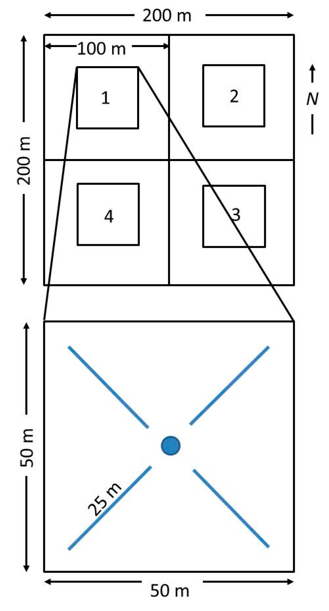
2.1. Field Location

The field investigation took place within the Boulder City Conservation Easement (BCCE), located in Eldorado Valley, Nevada (35°56.15′N, 114°53.93′W), with the field area extending south–southwest from just south of Boulder City, Nevada, for approximately 35 km (Figure 1). The DCP is split by U.S. Highway 95 into a north section (15,802 ha) and a south section (19,172 ha). An area of 1040 ha, designated by Boulder City for energy development (known as the Energy Zone), was not analyzed in this study. Eldorado Valley itself extends for about 20 km in the east-west direction and is bounded to the east by the Eldorado Mountains and to the west by McCullough Range. The valley extends for approximately 56 km in the north-south direction from Boulder City to Searchlight, Nevada. Elevation ranges from 521 m in Eldorado Dry Lake to 2152 m (McCullough Mountain).
The mean annual precipitation in Boulder City was 138 mm from 1931 to 2004 (Station 261071, Western Regional Climate Center, Reno, Nevada). August, with a mean monthly precipitation of 21.6 mm, is generally the wettest, while June, with a mean monthly rainfall of 2.7 mm, is driest. Mean annual temperature is 19.6 °C; July is the warmest month (mean maximum temperature of 32.5 °C), and January is the coolest month (mean minimum temperature of 0.5 °C). The dominant plant species are creosote bush (Larrea tridentate; LATR) and white bursage (Ambrosia dumosa; AMDU) [22]. Soils are typically stony calcareous alluvial sandy loams of the Arizo/Bitter Spring/Nickel complex at higher elevations and finer-grained McCullough/Rilito soils along axial washes, and distal fan and playa skirts.

2.2. LiDAR Data and Image Acquisition

Airborne LiDAR data were acquired on 15–19 October 2013 using a Chiroptera I (AHAB/Leica, Jönköping, Sweden) system mounted into a twin-engine Partenavia aircraft. Data were acquired at a repetition rate of 100–150 kHz, yielding a point density of 5–8 points/m2. Flight altitude was 600–900 m above ground, and flight speed averaged ~120 kt. The total survey area reported here was around 35,500 ha, split into four blocks to better accommodate changing terrain elevation and the repetition rate of the LiDAR instrument. GPS base stations (model Net R9, Trimble, Sunnyvale, CA, USA), recorded at 1-s intervals, operated during airborne missions and for system-calibration purposes. Static ground-control points for calibration were collected in the central portion of Eldorado Valley for vertical-elevation (slant range) comparison and correction. More than 450 points were acquired with an average of less than 5-m spacing using a dual-frequency GPS receiver (model R8, Trimble). With a LiDAR overflight, laser points that fell within 1 m of each ground-control point were compared using the least-squares method. The average difference between ground-control points and final LiDAR-derived vertical elevation was 3.3 cm. Results also show that 95% of errors in roll and pitch were smaller than 7 cm, equivalent to the lateral offset. These results are equivalent to the highest quality LiDAR data available (QL0), as specified by the U.S. Geological Survey [23].
LiDAR data processing and calibration were carried out using LiDAR Survey Suite (v. 2.09) to convert data into industry standard LAS (v. 1.2) file format. Software (Terra Solid, TerraScan, v. 014.28) was then used to merge segment files of individual flight lines into 226 individual (2 × 2 km) tiles to ease the computation load for data analysis and storage. All tiles were adjusted to true elevations using an interpolated Geoid model 2012A provided by National Geodetic Survey and calibrated using standard methods [24,25,26,27].
Airborne images were collected by Sanborn Map Co. (Colorado Springs, CO, USA) in March and April of 2014 at a flight height of ~3100 m above ground surface. Sanborn employed an UltraCam Eagle system to produce pan-sharpened 15.24-cm resolution images using panchromatic (20,010 × 13,080 pixels, 100.5 mm focal length, 5.2-μm pixel size) and multispectral (6670 × 4360 pixels, 100.5-mm focal length, 5.2-μm pixel size) cameras. Radiometric resolutions are 12 bit for both cameras; spectral-detection ranges are 410–730 nm (pan) for the panchromatic camera, and 440–520 nm (blue), 500–615 nm (green), 600–690 (red), and 710–830 (NIR) for the multispectral camera. Radiometric corrections and enhancements were applied by Sanborn, including gamma and color adjustments, shadow reduction, and haze reduction. Orthometric corrections were applied using proprietary software incorporating GPS/IMU mission data, geodetic ground control, and DEM to ensure ±0.3-m accuracy.

2.3. Field Measurements

As part of a separate effort conducted by a consulting firm located in Las Vegas, field crews set up 80 ground-based field plots for intensive surveys of plant diversity and richness, and the absence and presence of tortoise burrows and dimensions. These 4-ha plots were distributed across the LiDAR survey area using the Generalized Random Tessellation Stratified design (GRTS) [28,29] and georeferenced using a handheld GPS receiver (Trimble GeoExplorer 3000, accuracy 0.5 m). The experimental design for each plot (Figure 2) consisted of four 1-ha subplots (oriented as 2 × 2 ha for each field plot, except one, where only two subplots were established; 318 total). Subplots were then nested again into 50 × 50 m subplots, broken into four 25-m-long transects, starting 5 m from the center point of the subplot and radiating toward the corners of the subplot at 45, 135, 225, and 315 degrees. Vegetation cover was calculated as a percentage of the transect intersected by any shrub that crossed the vertical plane of the transect [30,31]. Gaps in vegetation were greater than 20 cm before recording as no vegetation cover. Each species was measured separately, even when overlapping. Bare ground was expressed as the inverse of total vegetation cover. Together with 16 transects at each of 80 plots, a total of 1248 transects were established with measurements of percent ground cover, basal diameters, and species.
Five of the 80 field plots were selected in this study as calibration plots: #2, #5, #19, #33, and #52 (Figure 1). These plots were chosen given their wide range of percent ground cover, from 9.2% at plot #52 to 23.7% at plot #33. At each of these five calibration plots, the northwest subplot (#1 in Figure 2) was identified, the original line transects were reestablished, and the following measurements were taken at each shrub that either intersected the line or was nearby: shrub species, shrub height, major and minor canopy diameters, and basal diameter. Shrubs within shrub islands were measured separately. GPS coordinates at the center of each shrub were recorded using a Trimble R8, with an error of 1–2 cm.
Canopy characteristics were measured for approximately 40 shrubs per calibration plot (213 in total). Height (H) was measured from the soil surface beneath the shrub to the approximate overall canopy top; canopy diameter (D) was determined in the maximum and minimum directions; and basal diameter (B) was measured in a single direction. To calculate canopy area and volume, we followed the methods outlined by Hamerlynck et al. [33]. Canopy area was calculated as A = π (D1/2) (D2/2), where D1 and D2 are diameters along major and minor semi-axes, respectively. Canopy volume (V) for Larrea was calculated as the frustum of an inverted, right circular cone (V = [1/3]πH[(D/2)2 + (B/2)2 + (D/2 + B/2)]. Canopy volume for Ambrosia is based on the ratio of H/D [33]. For conditions where H/D ≥ 1, volume was approximated as a prolate spheroid (V = [1/3]πH2[3(D/2) − H]), and when H/D < 1, volume was approximated as a hemisphere (V = [1/6]πH[3(D/2)2 + H2]). When canopy characteristics were compiled, we used canopy area as training sets for both LiDAR and aerial imagery measurements, and shrub height as a training set for LiDAR measurements.

2.4. Determining Shrub Presence and Canopy Characteristics

Estimates of shrub presence and canopy characteristics were tested using both LiDAR and aerial imagery. We posited that LiDAR returns would discriminate between ground surface and shrub, and provide data on shrub height and canopy volume, when appropriate. Aerial imagery distinguishes the tan/brown desert ground surface from the greener vegetation surface (~15 cm pixels) to approximately capture canopy diameter but not shrub height.
To identify whether a pixel overlaid a shrub (versus bare soil), we sought thresholds for the Normalized Difference Vegetation Index (NDVI) and the average reflectance (AVGr) of each band in the imagery (B, G, R, IR). A sensitivity analysis sequentially varied NDVI and AVGr across a wide range of values to determine if the spectral reflectance of pixels met the NDVI and AVGr thresholds. The algorithm was targeted onto the same LATR or AMDU shrubs measured in the field, yielding a root mean squared error (RMSE) between the observed and predicted canopy area. At least five contiguous pixels were needed to confidently detect a shrub; thus, for a single pixel with area = 0.023 m2 (15.24 cm on a side), the canopy area must have equaled or exceeded 0.1161 m2 (a square ~34.07 cm on a side). We used 400 combinations of NDVI and AVGr, calculating RMSE for each combination.
Once shrub locations were identified with aerial imagery, they were further assessed using data from the LiDAR. Here, we used commercially available software, LAStools [34], to reclassify each return in the point cloud as either ground or not ground, and then generated two 0.5 m rasters, one from ground-surface points and another from non-ground points. The ground-raster cells were determined by the average elevation value of points within the cell. For the non-ground raster, the maximum elevation point within each raster cell was assigned to that cell. Shrub height was determined by subtracting values from the two rasters, creating a new dataset with z-values representing height above ground. Finally, the shrub-height raster file was overlaid onto the aerial imagery, with shrub canopies identified using the algorithm described above. The highest coincident height value in the overlapping height file was assigned to each shrub. The identification of maximum shrub height is equivalent to Method 3, as discussed by Glenn et al. [35].

2.5. Establishing Geomorphic Parameters

The original data for terrain analysis—from the NRCS SSURGO Soil Survey Data (NV788 and NV755)—were reduced by removing terrain classes labeled bedrock or pediments, or specified as having a slope greater than 15%. Thus, we retained soil units. The remaining surface derivatives were all obtained using the 5-m LiDAR DEM and the Soil Inference Engine (ArcSIE) in ArcMap (v10.3) as developed by the USDA-NRCS [36].
ArcSIE was used to derive terrain indices directly from the DEM, including surface roughness, slope, curvature, and unipath wetness index. The Topographic Ruggedness Index (TRI) developed by Riley [37] is the root-mean-squared difference between the elevation of a cell and the moving mean elevation of the cells in a simple 3 × 3 neighborhood, using a 5-m DEM (square window of 15 m by 15 m); a low value indicates a smooth surface. Slope measures the steepness at a location, with output in percentage (i.e., 45 degrees = 100%). Curvature in planform is the shape of the slope surface in the horizontal (cross-slope) direction; positive values indicate convex shapes, and negative values indicate concave shapes. Finally, wetness indices are derived from a composite of flow direction and accumulation. First, flow direction assumes water moves toward the neighboring cell of steepest decent. Second, flow accumulation sums the total areas of upgradient cells. This Compound Topographic Index (CTI) divides the unipath flow-accumulation layer by slope gradient, where low values are dry and high values wet.
The surface-derivative algorithms use a modified Zevenbergen and Thorne [38] method that assumes the terrain surface can be modeled by a Lagrange polynomial. The Zevenbergen-Thorne method was applied separately to the four cardinal cells and four diagonal cells (eight surrounding cells); the average of the results from the two operations was used as the final result. We used a radius of 10 neighborhood cells in all cases [39].

2.6. Statistical Analyses

To determine the success of our approach for identifying individual shrubs, shrub area, and percent ground cover, we compared observed and predicted shrub areas using either a standard t-test or Mann-Whitney rank sum, depending on the assumption of normality (Shapiro-Wilk). Standard linear regression was used to relate observed (from line transects) and predicted (from imagery) percent ground cover and LiDAR-measured shrub heights; and nonlinear regression (Levenberg-Marquardt least squares) was used to relate imagery area to field-measured shrub height. Soil and vegetation characteristics, discussed above, were assigned to each tortoise burrow visually identified in the field by Clark County personnel. A table of these characteristics was compiled and used to create GIS masks that identified areas in the field site that met specific criteria (e.g., burrows only found in areas with certain slope or percent ground cover). All statistics are determined at 95% confidence.

3. Results and Discussion

3.1. Shrub Presence and Canopy Characteristics

The method used to identify an optimum combination of NDVI and AVGr thresholds from the imagery yielded an objective function (Figure 3a) showing where combinations led to lower RMSE. The region of minimal RMSE was rather large, however, occupying two combinations in the parameter space. One combination was found at NDVI ≥ 0.10 and AVGr ≤ 110–115, and the second combination from NDVI ≥ 0.12–0.40 and AVGr ≤ 120–125. However, when applying these values to areas with larger rocks or perennial grasses, which could be viewed in aerial imagery, these features were falsely classified as shrubs. Using NDVI ≥ 0.12 and AVGr ≤ 111 (as shown on the circle on Figure 3a) provided accurate estimates of shrub area (compared to observed shrub area) and a minimum level of false identifications; thus, we used these values throughout the analysis with confidence that a shrub occupied a particular spatial location.
This combination of parameters led to a scatterplot of observed versus predicted canopy area (Figure 3b), showing only a slight overestimation of canopy area (regression slope = 1.0826, n = 163) but excellent linearity and low estimation error (R2 = 0.9282 and standard error = 0.669 m2). Results of the Mann-Whitney rank sum test comparing the two samples indicate no statistical difference between the two (U = 12,257; p = 0.228). Figure 4 shows a direct comparison between shrubs identified in the aerial imagery and shrubs estimated using the algorithm described (we show only site #39 as an example; other sites were similar). All shrubs measured in the field were identified using this analysis, demonstrating that the method—used to identify shrubs across the entire 35,500 ha area—provides a robust means of identifying the presence of shrubs in Eldorado Valley.

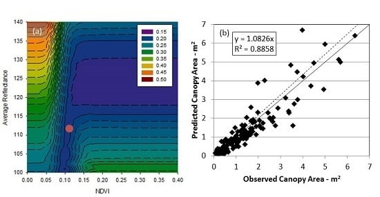
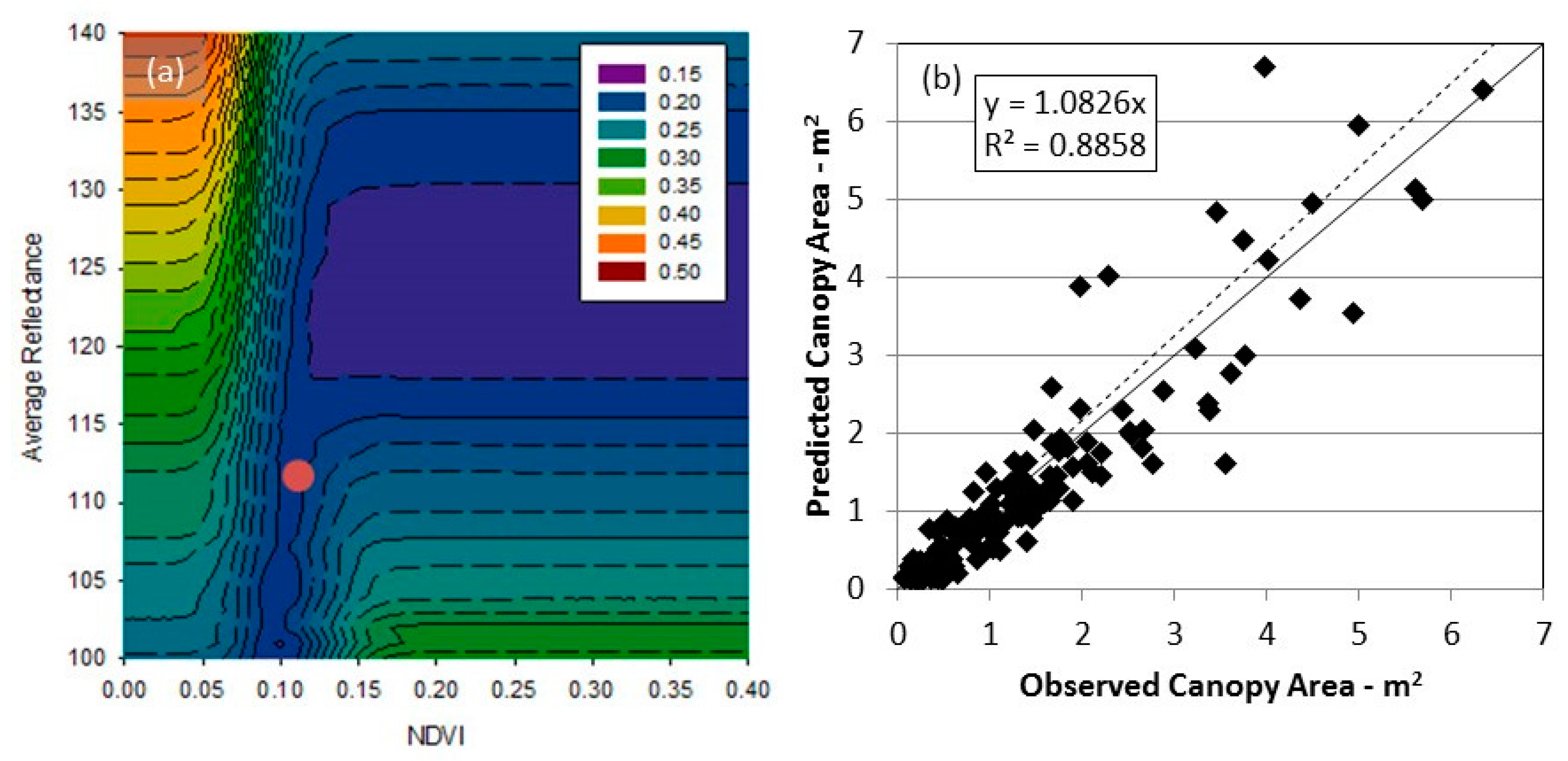
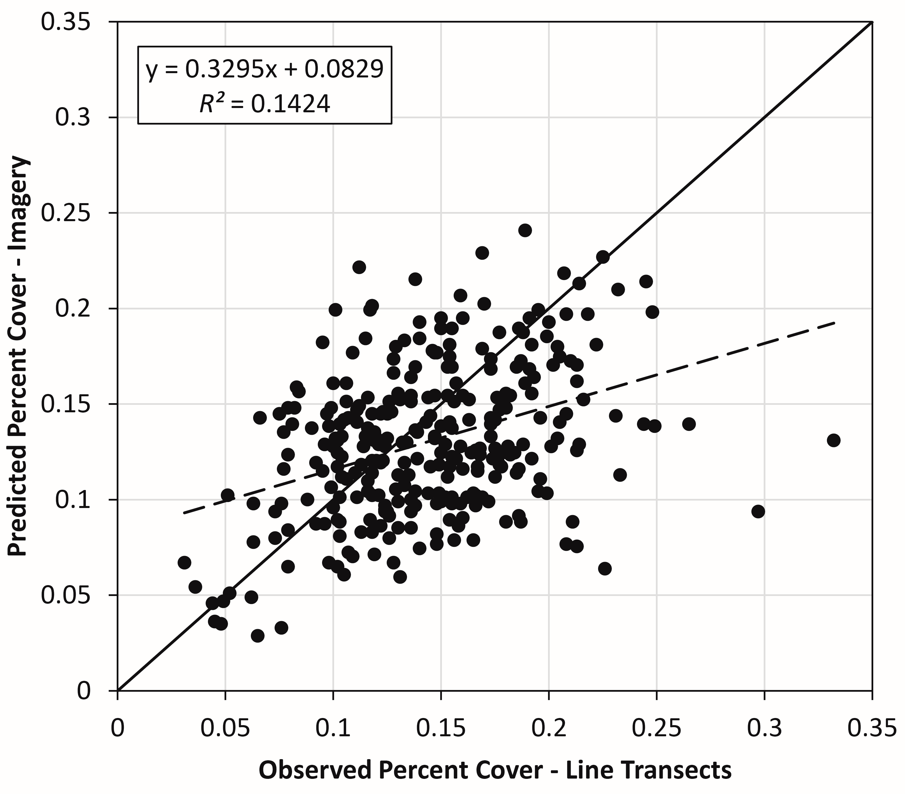
3.2. Comparison between Imagery-Derived Estimates and Ground-Based Measurements of Canopy Area and Percent Coverage

Figure 5 shows a comparison between observed percent ground cover from the line transects (16 transects at all 80 survey plots shown in Figure 1) versus predicted percent ground cover determined from aerial imagery for all surveyed subplots across the field site. Considerable scatter was observed between the observed and predicted cover, as well as a dependence on a small number of potential outliers located in the southern portion of the site, where lighter-colored soils reduced the NDVI and hence the predicted percent cover from imagery. A t-test indicates that the two datasets are statistically different (p < 0.001), which is not unexpected; the observed percent cover is a sample of a population and thus subject to considerable variability, determined only by whether a particular shrub overlays the transect. The predicted percent cover, on the other hand, is a measure of the entire population of shrubs found within the 1-ha plot.
Another factor to consider is the resolution of the aerial imagery and its impact on the minimum estimated canopy area, which was established at 0.1161 m2 (34 cm × 34 cm), when compared to the line-transect method. (All shrubs intersecting the line transect, regardless of size (which was not determinable from the survey), were included in the observed percent cover.) To determine whether shrubs with areas smaller than 0.1161 m2 could significantly increase the total canopy area, we binned LATR and AMDU.
Shrubs identified inside all 50-m × 50-m subareas, according to their relative canopy areas, so that we can assess whether shrubs below detection could be estimated. Figure 4a,b shows the distribution of LATR and AMDU shrubs, respectively. When plotting the number of shrubs in logarithmic space against canopy area, the linearity of the functions is apparent, allowing us to estimate the number of shrubs—and associated area—that are represented in the canopy area bin, which is smaller than 0.1161 m2. We noted a deviation from log linearity in the LATR shrubs (open squares in Figure 6a), which necessitated a second regression line. Using regression lines and solving for number of shrubs at the smallest bin (i.e., <0.1161 m2), we estimated that nearly 13,900 LATR and 47,750 AMDU shrubs could potentially exist in the 318 subplots. By summing the canopy area times the number of shrubs for each bin, and including these smallest shrubs, we estimated the total canopy area occupied by LATR and AMDU (80,946 m2 and 27,769 m2, respectively) and percent ground cover (10.36% and 3.55%, respectively) within the subplots, or a total estimated percent ground cover of 13.92%. This estimate compares favorably with the 14.52% estimated from the 1272 line transects. Including the small shrubs into the predicted percent cover (Figure 5) would have increased the regression slope (to 0.3295) and offset (to 0.0829) but not the value of R2.

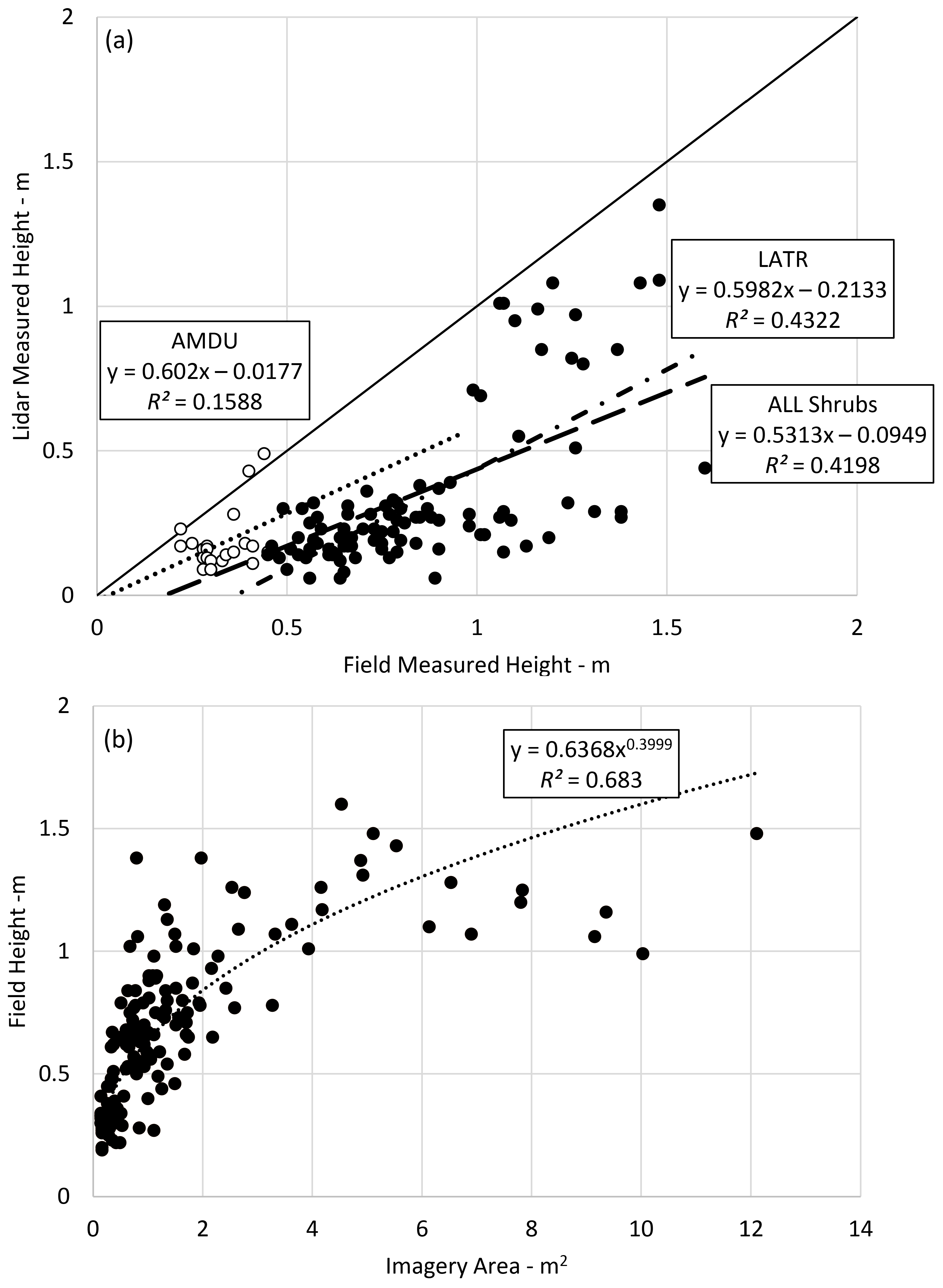
3.3. Comparison between LiDAR-Derived Estimates and Ground-Based Measurements of Shrub Height

Figure 7a shows the results of LiDAR-measured heights when compared to field-measured heights of the same shrubs (n = 121; note that measured shrubs too short to be detected by LiDAR are not included). The LiDAR clearly underestimates shrub height, which is not surprising given the open-canopy structure of both shrubs, LATR in particular, and the relatively low probability of the maximum LiDAR return intensity focusing on the highest branch of the shrub when the LiDAR pulse rate is ~100–150 kHz. Using slope of the linear-regression line as an indication of the average underestimation, the LiDAR height was ~60% of the true height of LATR and AMDU shrubs measured in the field, with correlation coefficients that provide only moderate confidence in predictability (R2 = 0.4198; RMSE = 0.201). Another approach for estimating heights of the nearly 62 million shrubs across the survey area is to use the aerial imagery-derived shrub area as a predictor of shrub height. Figure 7b compares the imagery-derived area and field-measured shrub height, including a power-law relationship (n = 152) that captures the majority of the variability observed in the field-measured height. When comparing field-measured height and predicted height using this power-law function, the results (RMSE = 0.194 cm) indicate an improvement over those shown in Figure 7a. Therefore and subsequently, we estimated shrub height using only the aerial imagery-derived canopy area and not the LiDAR returns as the predictor.

3.4. Correlating Soil and Vegetation Characteristics to Observed Burrows

Tables S1–S3 (found in the Supplementary Materials) provide data for the ~100 tortoise burrows that were observed during previous (and unrelated to this project) field surveys. Data include general site characteristics, soil and landscape characteristics, and vegetation characteristics. For the purposes of this study, we assessed whether selected characteristics (e.g., roughness, aspect, slope percent, elevation, and percent ground cover) could be used as criteria for when tortoise burrows are present. Here, the DEMs used for criteria a–d were determined at 5-m resolution, and percent ground cover (criteria e) was determined at 10-m resolution (higher resolution led to unacceptable variability). The following criteria were based on the terrain features where burrows were identified:
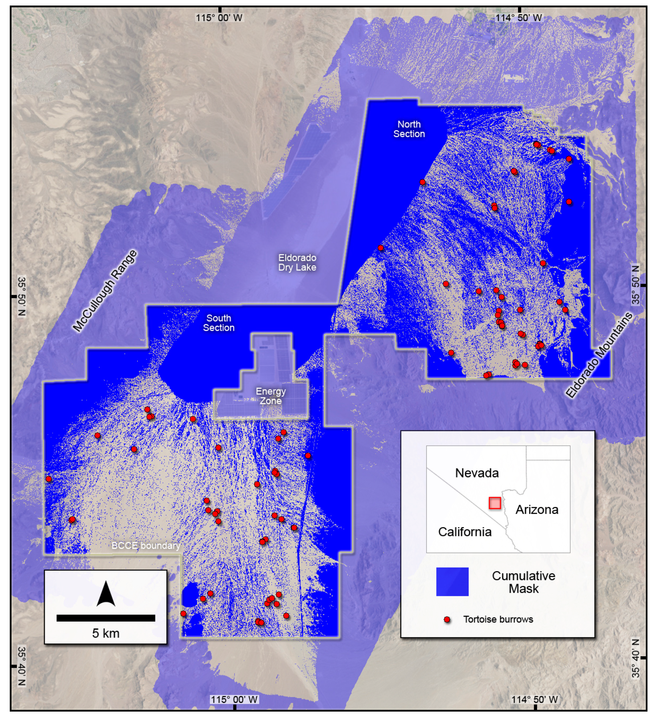
  • Burrows found only on surfaces with roughness < 1.788;
  • Burrows found only on slopes shallower than 4.6%;
  • Burrows found only when aspect < 126° or >222°; north is 0° rotated clockwise;
  • Burrows found only on land with elevation between 559 and 845 m above mean sea level;
  • Approximately 25% of burrows found in areas with percent ground cover < 10%.
Land curvature had no discernable correlation to the presence of burrows. Moreover, we found that ~60% of burrows were located on aprons and piedmonts, and 95% of burrows located on aprons, piedmonts, or remnants. With such a high percentage of burrows on these surfaces, we concluded that the geomorphic description was not an effective discriminatory variable.
For each of the five criteria listed above, we created a mask that was overlain atop the field site. When added, the masks show a cumulative effect on areas where tortoise burrows are less likely to be present—or, more specifically, where tortoise burrows have not been observed in the past. Figures S1–S5 (found in the Supplementary Materials) represent the cumulative effect of the masks and are presented in the same order as those listed above; Figure 8 shows the final mask, with all earlier masks shown in dark blue. The results show the effect of steeper mountainous areas mostly on roughness and slope—though portions of these areas are outside of the BCCE boundaries—with important contributions from the aspect; it is clear, however, that percent ground cover has the most significant effect. In Figure S5, the contours of percent ground cover from 0% to 10% are most pronounced near the intersection of the mountain front and alluvial fan, with color shading on the alluvial fan showing a pattern that follows drainages on the fan surface. For example, on the northern portion of the field site, large areas with percent ground cover ~5% are most likely mantled with thin soils or petrocalcic horizons that prevent robust vegetation growth and/or hinder burrowing; thus, these areas are less favorable. Areas that visually appear to show tortoise burrows overlying zones of low percent ground cover (Figure S5) are an artifact of the scaling of the figure and show the high spatial variability of shrub growth in this desert valley.
Figure 9a shows the relative percent of each criterion when assessed separately; Figure 9b shows the cumulative effect of successively adding each criterion (A through E). Several of the masks overlap one another, especially toward the mountain front, so that the cumulative area of the BCCE mask (55.9%) is less than the sum of the individual masks (86.89%). Somewhat surprisingly, a large area in the southwest portion of the BCCE appears to pass the criteria, but burrows were not observed, leading to the possibility that other characteristics (e.g., soil thickness, soil structure) are important and worthy of further consideration. Published authorized by the Director, Bureau of Economic Geology.

4. Conclusions

The use of LiDAR and aerial imagery presented some challenges in this desert environment, but the approaches taken here have produced a rich dataset that can be used for several purposes, including assessing potential burrow locations for G. agassizii. Specific conclusions are as follows:
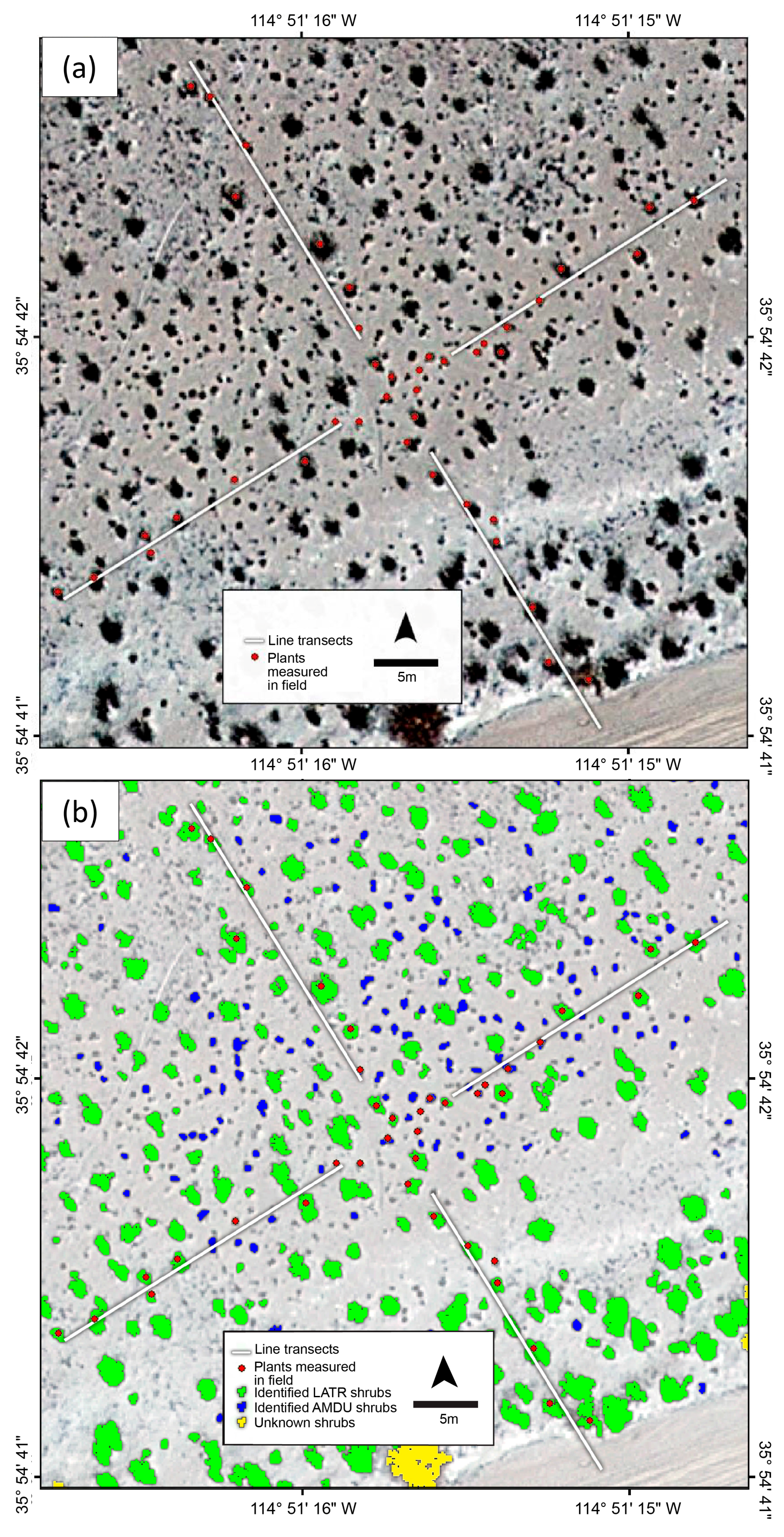
  • The 80 field plots with line transects provided excellent data to which we could compare imagery-derived canopy area and percent ground cover. Comparisons of canopy areas of individual shrubs (field-measured versus imagery-estimated) were excellent and highly correlated (R2 = 0.9282), but comparisons broke down when comparing percent ground cover derived from line transects versus imagery. This is because the line transects only sample a small number of shrubs without measurements of canopy areas, whereas the imagery yielded canopy areas of every shrub in the target area greater than 0.1161 m2.
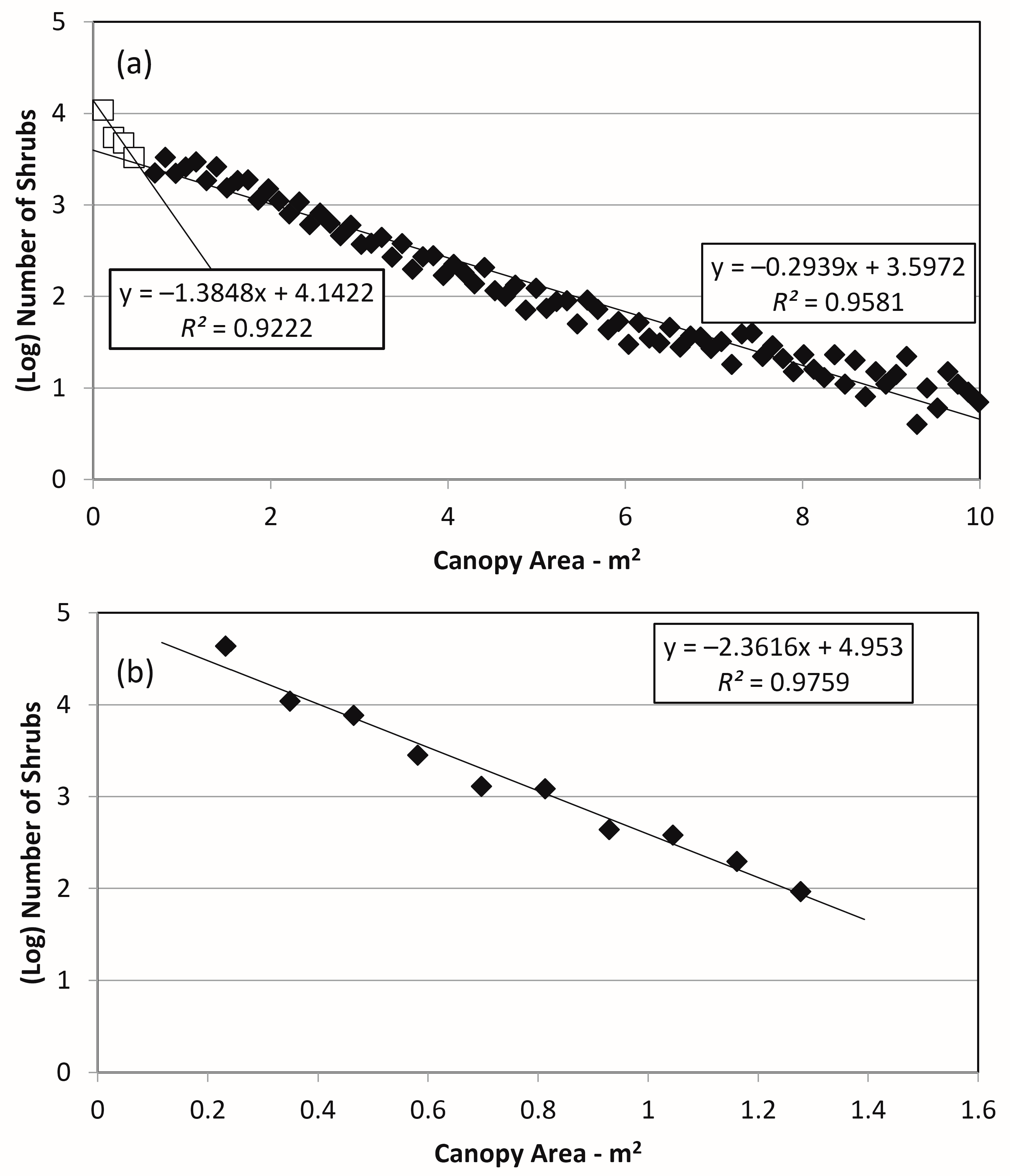
  • We estimated the number of smaller shrubs below a “detection limit” of 0.1161 m2 and found that the cumulative canopy areas for these small shrubs improved the comparison of survey-wide, average percent ground cover. Our estimate of a percent ground cover of 13.92% compares favorably with the 14.52% estimated from the 1248 line transects.
  • Use of LiDAR returns for estimating canopy height low-biased the results by ~60%. Underestimation using LiDAR has been reported by others [40,41,42]. Specifically, Sankey et al. [42] conducted field vegetation surveys, including L. tridentata shrubs, in which shrub height and area were measured. With repeated measurements using a ground-based LiDAR system (over both time and multiple scanning locations), they noted an underestimation of LiDAR-based L. tridentata shrub height of approximately 32% for single-scan positions and 16% for multiple-scan locations. Luscombe et al. [41] compared airborne LiDAR to terrestrial laser scanning in a peatland ecosystem and also found a systematic underestimation of canopy heights, as measured relative to mean sea level (not shrub-specific heights).
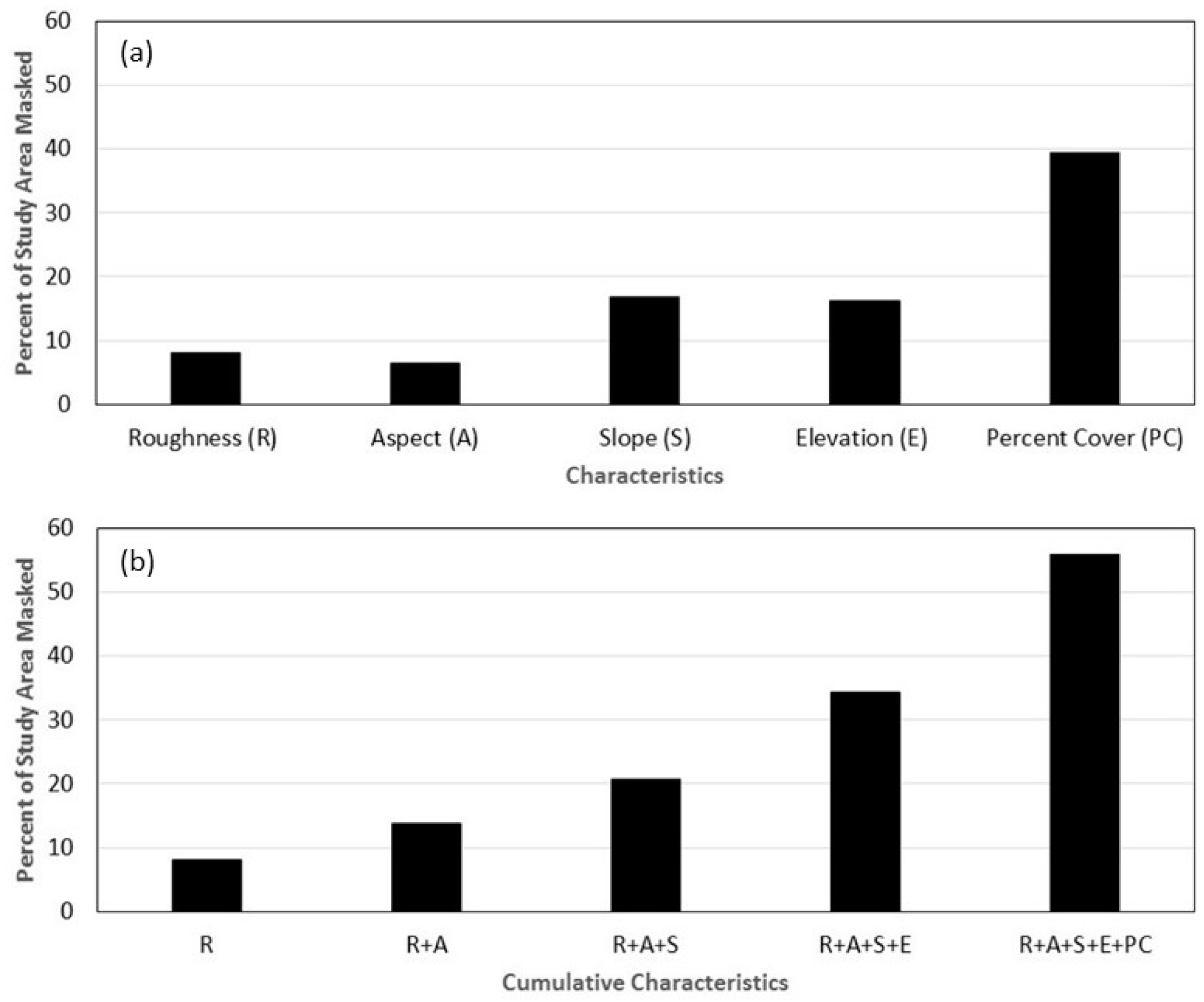
  • The use of aerial imagery for estimating vegetation characteristics, and of LiDAR data for estimating terrain characteristics, leveraged the benefits of both methods, yielding information that helps identify areas where tortoise burrows are more likely to be found. Though not a modeling approach per se, we showed that 55.9% of the 35,500-ha area is less likely to be favored for burrowing, using only five vegetation and terrain characteristics (roughness, aspect, slope percent, elevation, and percent ground cover). Other factors such as soil friability, distance to roads, and invasive cover could further refine these potential locations.
  • The success of the remote-sensing work reported here on identifying burrows is strongly dependent on the visual identification of burrows for ground truthing (i.e., portions of the study were masked because of a lack of visually identified burrows, not because burrows were verified as being absent). Therefore, it is important to emphasize the need for ecological data to better refine those locations most likely to host tortoise burrows and, hence, to prioritize areas to search.
    We recognize that habitat preferences for the desert tortoise (Gopherus agassizii) are dependent on many factors not considered in this study, particularly forage, suitability for breeding, refuge, etc.; thus, the results presented here should be taken in their proper context and applied to the challenging issue of habitat suitability with caution.

Supplementary Materials

The following are available online at www.mdpi.com/2072-4292/9/5/458/s1. Figure S1. Map showing surface roughness overlain atop the field site. Colored areas are those with roughness > 1.788 and areas without color are <1.788. The BCCE is shown in a dark outline and red dots indicate locations with visual confirmation of tortoise habitats; Figure S2. Map showing a double overlay of surface roughness and aspect overlain atop the field site. Colored areas include those with roughness > 1.788 and aspect between 126° and 222°. The BCCE is shown in a dark outline and red dots indicate locations with visual confirmation of tortoise habitats; Figure S3. Map showing a cumulative overlay of surface roughness, aspect and slope, overlain atop the field site. Colored areas include those with roughness > 1.788, aspect between 126° and 222°, and slope > 4.6%. The BCCE is shown in a dark outline and red dots indicate locations with visual confirmation of tortoise habitats; Figure S4. Map showing a cumulative overlay of surface roughness, aspect, slope, and elevation, overlain atop the field site. Colored areas include those with roughness > 1.788, aspect between 126° and 222°, slope > 4.6%, and elevation between 450 and 1350 m a.s.l. The BCCE is shown in a dark outline and red dots indicate locations with visual confirmation of tortoise habitats; Figure S5. Map showing a cumulative overlay of surface roughness, aspect, slope, elevation, and percent ground cover, overlain atop the field site. Colored areas include those with roughness > 1.788, aspect between 126° and 222°, slope > 4.6%, elevation between 450 and 1350 m a.s.l., and vegetation cover > 10%. The BCCE is shown in a dark outline and red dots indicate locations with visual confirmation of tortoise habitats; Table S1. General description of observed tortoise burrows; Table S2. Soil and landscape attributes in immediate vicinity of observed tortoise burrows; Table S3. Vegetation characteristics in immediate vicinity of observed tortoise burrows.

Acknowledgments

This study was sponsored by the Clark County Desert Conservation Program, Las Vegas, Nevada, under contracts CBE 603383-14 and CBE 604014-16. We acknowledge the assistance of Larry Mata, Lee Bice, and Scott Cambrin of the Clark County Desert Conservation Program; field assistance from Douglas Merkler of the USDA-NRCS; and LiDAR data collection and analysis support by Aaron Averett, Tiffany Caudle, Rebecca Brown, and John Hupp, all of the Bureau of Economic Geology, Jackson School of Geosciences, University of Texas at Austin.

Author Contributions

M.H.Y. conceived of the project, performed field work and wrote the paper; J.H.A. performed field work, developed algorithms, and analyzed aerial and LiDAR data; T.G.C. analyzed geomorphic attributes, performed field work and contributed to sections of the paper; K.S. conducted LiDAR survey, analyzed LiDAR data and contributed to sections of the paper.

Conflicts of Interest

The authors declare no conflict of interest. The founding sponsors had no role in the writing of the manuscript, or in the decision to publish the results.

References

  1. U.S. Endangered Species Act of 1973. Available online: http://www.nmfs.noaa.gov/pr/pdfs/laws/esa.pdf (accessed on 1 May 2017).
  2. U.S. Fish and Wildlife Service. Endangered and threatened wildlife and plants: Determination of threatened status for the Mojave population of the desert tortoise. Federal Register 1990, 55, 12178–12191. [Google Scholar]
  3. Abella, S.R.; Berry, K.H. Enhancing and restoring habitat for the desert tortoise. J. Fish Wildl. Manag. 2016, 7, 255–279. [Google Scholar] [CrossRef]
  4. Belnap, J.; Warren, S.D. Patton’s tracks in the Mojave Desert, USA: An ecological legacy. Arid Land Res. Manag. 2002, 16, 245–258. [Google Scholar] [CrossRef]
  5. Caldwell, T.G.; McDonald, E.V.; Young, M.H. Soil disturbance and hydrologic response at the National Training Center, Ft. Irwin, California. J. Arid Environ. 2006, 67, 456–472. [Google Scholar] [CrossRef]
  6. Efroymson, R.A.; Peterson, M.J.; Jones, D.S.; Suter, G.W. The Apache Longbow-Hellfire missile test at Yuma Proving Ground: Introduction and problem formulation for a multiple stressor risk assessment. Human Ecol. Risk Assess. 2008, 14, 854–870. [Google Scholar] [CrossRef]
  7. Caldwell, T.G.; McDonald, E.V.; Young, M.H. The seedbed microclimate and active revegetation of disturbed lands in the Mojave Desert. J. Arid Environ. 2009, 73, 563–573. [Google Scholar] [CrossRef]
  8. Webb, R.H.; Belnap, J.; Thomas, K.A. Natural Recovery from Severe Disturbance in the Mojave Desert. In The Mojave Desert: Ecosystem Processes and Sustainability; Webb, R.H., Fenstermaker, L.F., Heaton, J.S., Hughson, D.L., McDonald, E.V., Eds.; University of Nevada Press: Reno, NV, USA, 2009; pp. 343–377. [Google Scholar]
  9. Hernandez, R.R.; Easter, S.B.; Murphy-Mariscal, M.L.; Maestre, F.T.; Tavassoli, M.; Allen, E.B.; Barrows, C.W.; Belnap, J.; Ochoa-Hueso, R.; Ravi, S.; et al. Environmental impacts of utility-scale solar energy. Renew. Sust. Energ. Rev. 2014, 29, 766–779. [Google Scholar] [CrossRef]
  10. Berry, K.H.; Coble, A.A.; Yee, J.L.; Mack, J.S.; Perry, W.M.; Anderson, K.M.; Brown, M.B. Distance to human populations influences epidemiology of respiratory disease in desert tortoises. J. Wildl. Manag. 2015, 79, 122–136. [Google Scholar] [CrossRef]
  11. Berry, K.H.; Yee, J.L.; Coble, A.A.; Perry, W.M.; Shields, T.A. Multiple factors affect a population of Agassiz’s Desert Tortoise (Gopherus agassizii) in the northwestern Mojave Desert. Herpetol. Monogr. 2013, 27, 87–109. [Google Scholar] [CrossRef]
  12. Baxter, R.G. Patial distribution of desert tortoises (Gopherus agassizii) at Twentynine Palms, California: Implications for relocations. In Management of Amphibians, Reptiles, and Small Mammals in North America; Szoro, R.C., Siverson, K.E., Patton, D.R., Eds.; USDA: Washington, DC, USA, 1988; pp. 180–189. [Google Scholar]
  13. Lovich, J.E.; Daniels, R. Environmental characteristics of desert tortoise (Gopherus agassizii) burrow locations in an altered industrial landscape. Chelonian Conserv. Biol. 2000, 3, 714–721. [Google Scholar]
  14. Riedle, J.D.; Averill-Murray, R.C.; Lutz, C.L.; Bolen, D.K. Habitat use by desert tortoises (Gopherus agassizii) on alluvial fans in the Sonoran Desert, south-central Arizona. Copeia 2008, 2, 414–420. [Google Scholar] [CrossRef]
  15. Bergen, K.M.; Goetz, S.J.; Dubayah, R.O.; Henebry, G.M.; Hunsaker, C.T.; Imhoff, M.L.; Nelson, R.F.; Parker, G.G.; Radeloff, V.C. Remote sensing of vegetation 3-D structure for biodiversity and habitat: Review and implications for LiDAR and radar spaceborne missions. J. Geophys. Res. Biogeosci. 2009, 114. [Google Scholar] [CrossRef]
  16. Galik, C.S. Contributions of LiDAR to Ecosystem Service Planning and Markets: Assessing the Costs and Benefits of Investment. Available online: https://nicholasinstitute.duke.edu/ecosystem/publications/contributions-lidar-ecosystem-service-planning-and-markets-assessing-costs-and-benefits (accessed on 1 May 2017).
  17. Harpold, A.A.; Marshall, J.A.; Lyon, S.W.; Barnhart, T.B.; Fisher, B.A.; Donovan, M.; Brubaker, K.M.; Crosby, C.J.; Glenn, N.F.; Glennie, C.L.; et al. Laser vision: LiDAR as a transformative tool to advance critical zone science. Hydrol. Earth Syst. Sci. 2015, 19, 2881–2897. [Google Scholar] [CrossRef]
  18. Lefsky, M.A.; Cohen, W.B.; Parker, G.G.; Harding, D.J. LiDAR remote sensing for ecosystem studies. Bioscience 2002, 52, 19–30. [Google Scholar] [CrossRef]
  19. Goetz, S.J.; Steinberg, D.; Betts, M.G.; Holmes, R.T.; Doran, P.J.; Dubayah, R.; Hofton, M. LiDAR remote sensing variables predict breeding habitat of a Neotropical migrant bird. Ecology 2010, 91, 1569–1576. [Google Scholar] [CrossRef] [PubMed]
  20. Catano, C.P.; Angelo, J.J.; Stout, I.J. Sample grain influences the functional relationship between canopy cover and gopher tortoise (Gopherus polyphemus) burrow abandonment. Chelonian Conserv. Biol. 2014, 13, 166–172. [Google Scholar] [CrossRef]
  21. Flaherty, S.; Lurz, P.W.W.; Patenaude, G. Use of LiDAR in the conservation management of the endangered red squirrel (Sciurus vulgaris L.). J. Appl. Remote Sens. 2014, 8. [Google Scholar] [CrossRef]
  22. Rundel, P.; Gibson, A.C. Ecological Communities and Processes in a Mojave Desert Ecosystem: Rock Valley, Nevada; Cambridge University Press: New York, NY, USA, 2005. [Google Scholar]
  23. Heidemann, H.K. LiDAR Base Specification. Available online: https://dx.doi.org/10.3133/tm11B4 (accessed on 1 May 2017).
  24. Schenk, T. Modeling and Analyzing Systematic Errors in Airborne Laser Scanners; Ohio State University: Columbus, OH, USA, 2001. [Google Scholar]
  25. Habib, A.; Bang, K.I.; Kersting, A.P.; Chow, J. Alternative methodologies for LiDAR system calibration. Remote Sens. 2010, 2, 874–907. [Google Scholar] [CrossRef]
  26. Wehr, A. LiDAR systems and calibration. In Topographic laser Ranging and Scanning; Shan, J., Toth, C.K., Eds.; CRC Press: Boca Raton, FL, USA, 2009. [Google Scholar]
  27. Toth, C.K. Calibrating airborne LiDAR systems. In Proceedings of the ISPRS Commission II Symposium, Xi’an, China, 20–23 August 2002. [Google Scholar]
  28. Barabesi, L.; Fattorini, L. Random versus stratified location of transects or points in distance sampling: Theoretical results and practical considerations. Environ. Ecol. Stat. 2013, 20, 215–236. [Google Scholar] [CrossRef]
  29. Stevens, D.L.; Osen, A.R. Variance estimation for spatially balanced samples of environmental resources. Environmetrics 2003, 14, 593–610. [Google Scholar] [CrossRef]
  30. Elzinga, C.L.; Salzer, D.W.; Willoughby, J.W. Measuring and Monitoring Plant Populations; U.S. Bureau of Land Management: Denver, CO, USA, 1998.
  31. Greig-Smith, P. Quantitative Plant Ecology, 3 ed.; University of California Press: Los Angeles, CA, USA, 1983. [Google Scholar]
  32. Knight and Leavitt Associates. Vegetation Data for Desert Tortoise Occupancy Covariate Monitoring Project at the Boulder City Conservation Easement. Available online: http://www.clarkcountynv.gov/airquality/dcp/Documents/Library/symposium/2016/9-Vegetation%20Data%20for%20Desert%20Tortoise%20Occupancy%20Covariate%20Monitoring-2016.pdf (accessed on 1 May 2017).
  33. Hamerlynck, E.P.; McAuliffe, J.R.; McDonald, E.V.; Smith, S.D. Ecological responses of two Mojave Desert shrubs to soil horizon development and soil water dynamics. Ecology 2002, 83, 768–779. [Google Scholar] [CrossRef]
  34. Isenburg, M. LAStools—Efficient Tools for LiDAR Processing. Available online: http://lastools.org (accessed on 31 March 2017).
  35. Glenn, N.F.; Spaete, L.P.; Sankey, T.T.; Derryberry, D.R.; Hardegree, S.P.; Mitchell, J.J. Errors in LiDAR-derived shrub height and crown area on sloped terrain. J. Arid Environ. 2011, 75, 377–382. [Google Scholar] [CrossRef]
  36. Shi, X. ArcSIE Toolbox for Digital Soil Mapping, v 10.2.105; Dartmouth College: Hanover, NH, USA, 2013. [Google Scholar]
  37. Riley, S.J. A Terrain Ruggedness Index (TRI) that quantifies topographic heterogeneity Intermt. J. Sci. 1999, 5, 23–27. [Google Scholar]
  38. Zevenbergen, L.W.; Thorne, C.R. Quantitative analysis of land surface topography. Earth Surf. Process. Landf. 1987, 12, 47–56. [Google Scholar] [CrossRef]
  39. Shi, X.; Zhu, A.X.; Burt, J.; Choi, W.; Wang, R.X.; Pei, T.; Li, B.L.; Qin, C.Z. An experiment using a circular neighborhood to calculate slope gradient from a DEM. Photogramm. Eng. Remote Sens. 2007, 73, 143–154. [Google Scholar] [CrossRef]
  40. Streutker, D.R.; Glenn, N.F. LiDAR measurement of sagebrush steppe vegetation heights. Remote Sens. Environ. 2006, 102, 135–145. [Google Scholar] [CrossRef]
  41. Luscombe, D.J.; Anderson, K.; Gatis, N.; Wetherelt, A.; Grand-Clement, E.; Brazier, R.E. What does airborne LiDAR really measure in upland ecosystems? Ecohydrology 2015, 8, 584–594. [Google Scholar] [CrossRef]
  42. Sankey, J.B.; Munson, S.M.; Webb, R.H.; Wallace, C.S.A.; Duran, C.M. Remote sensing of Sonoran Desert vegetation structure and phenology with ground-based LiDAR. Remote Sens. 2015, 7, 342–359. [Google Scholar] [CrossRef]
Figure 1. Survey area superimposed on elevation (shown in color). The BCCE is shown in the gray outline; green dots are line transect survey plots; red dots are observed tortoise burrows; and yellow circles represent the location of designated plots for field vegetation measurements. Numbers refer to calibration plots used in the study.
Remotesensing 09 00458 g001
Figure 2. Layout of nested-vegetation survey locations for field validation in each of the 80 field plots [32].
Remotesensing 09 00458 g002
Figure 3. (a) Objective function showing RMSE as function of NDVI and AVGr; (b) scatterplot showing comparison between observed and predicted canopy areas for NDVI ≥ 0.12 and AVGr ≤ 111, as also seen in red dot shown on (a). In (b), the solid line represents the 1:1 line and the dashed line represents the regression line (significant at p < 0.001).
Remotesensing 09 00458 g003
Figure 4. (a) Observed and (b) predicted shrubs for Site #2, used as an example of other sites. White bars represent line transect locations; red dots represent plants measured in the field; green shapes represent LATR shrubs; and blue shapes represent AMDU shrubs, as identified by the algorithm.
Remotesensing 09 00458 g004
Figure 5. Scatterplot of observed versus predicted percent vegetation cover. Observed percent vegetation area is an average of measurements taken at four line transects in each subarea. Predicted canopy area is estimated from the imagery at NDVI ≥ 0.12 and AVGr ≤ 111. Solid line is 1:1 line; dashed line is regression line (significant at p < 0.001).
Remotesensing 09 00458 g005
Figure 6. Log number of shrubs in different size classes, shown on X-axis, for (a) LATR and (b) AMDU. Solid lines are (log) linear-regression lines. Note differences in X-axis range. Individual bins are 0.1161 m2, but the X-axis scale is shown as a round number to facilitate viewing. Regression lines significant at p < 0.001.
Remotesensing 09 00458 g006
Figure 7. (a) Comparison between field-measured and LiDAR-measured heights of LATR and AMDU shrubs; (b) field-measured height as a function of imagery-derived area for all shrubs. In (a), the solid line is the 1:1 line; the dashed/dotted line is for LATR, the dotted line is for AMDU, and the long-dashed line is for all shrubs.
Remotesensing 09 00458 g007
Figure 8. Map showing a cumulative overlay of all five criteria, each shown in blue. Areas without color (grey is the background imagery) have met all the criteria. The BCCE is shown as a gray outline, and red dots indicate locations with visual confirmation of tortoise burrows.
Remotesensing 09 00458 g008
Figure 9. Bar charts showing (a) percent of study area masked as favorable locations for burrows, as a function of terrain and vegetation characteristics; and (b) the cumulative effect of the characteristics on the percent of study area masked.
Remotesensing 09 00458 g009

