
Mapping Reflectance Anisotropy of a Potato Canopy Using Aerial Images Acquired with an Unmanned Aerial Vehicle


 ,
,  and
and
Abstract
:
1. Introduction
2. Materials and Methods
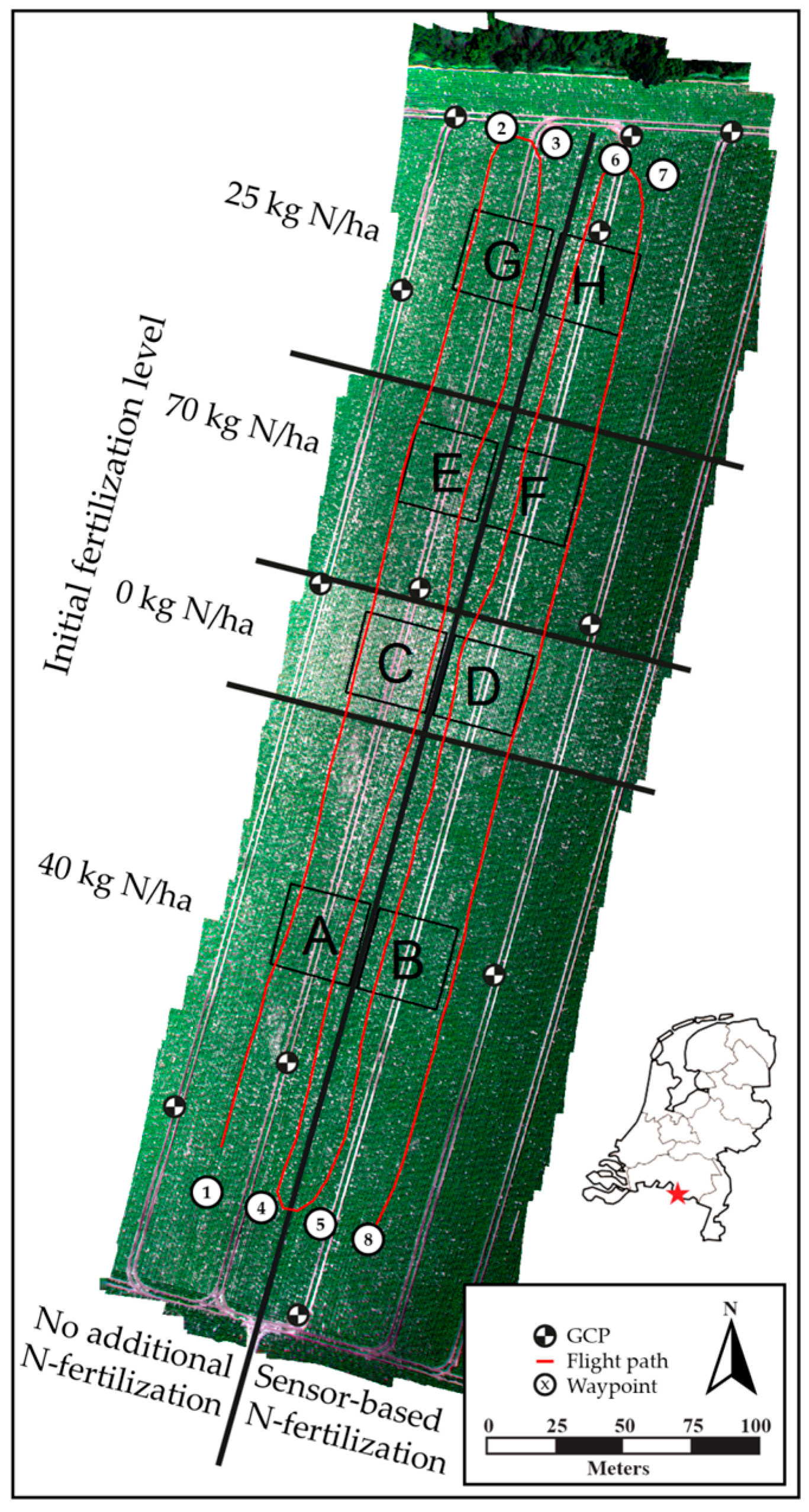
2.1. Study Area
2.2. UAV Flights
2.3. Spectral Measurements
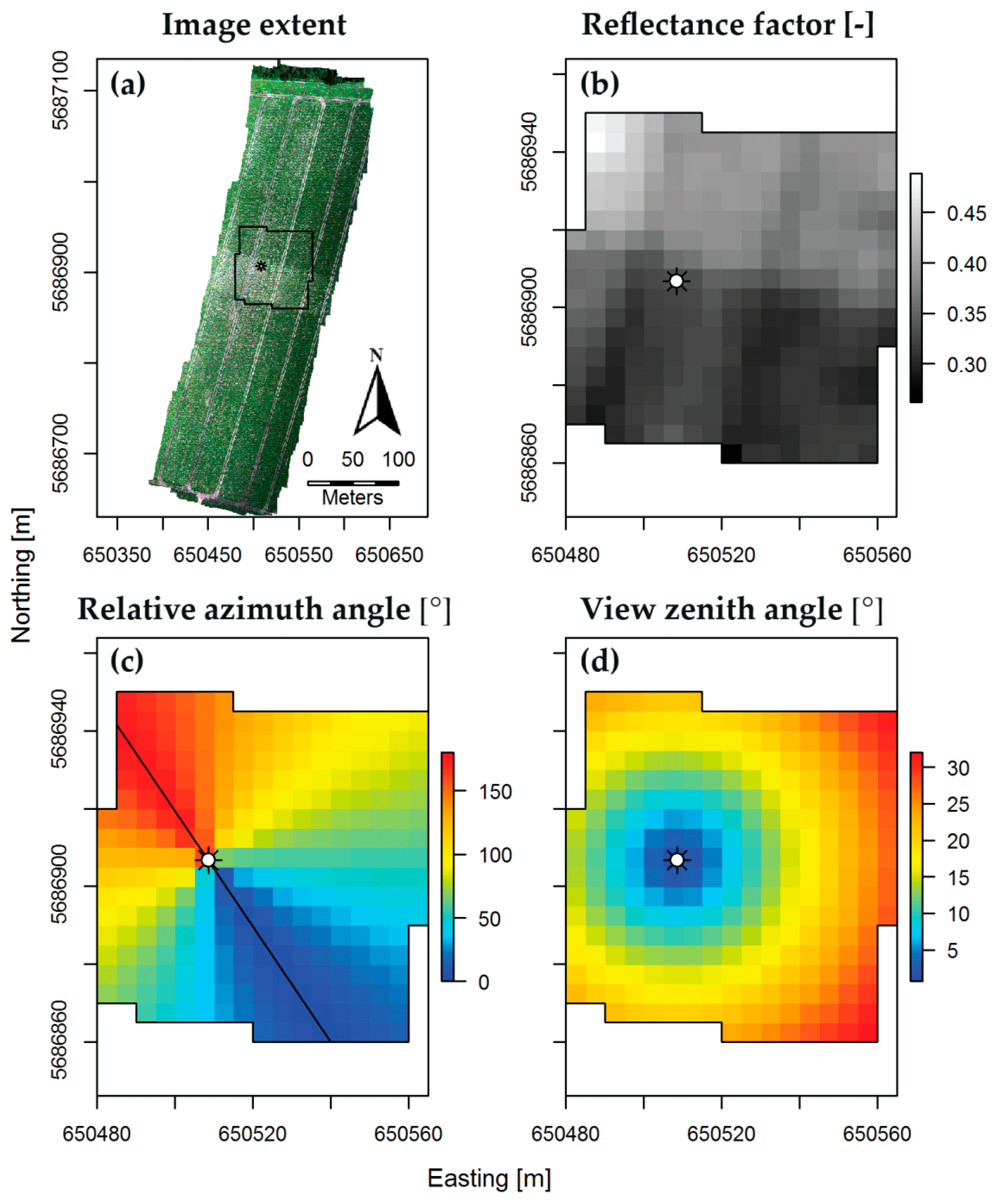
2.4. Orthorectification and Measurement Geometry
2.5. Data Analysis and Visualization
3. Results
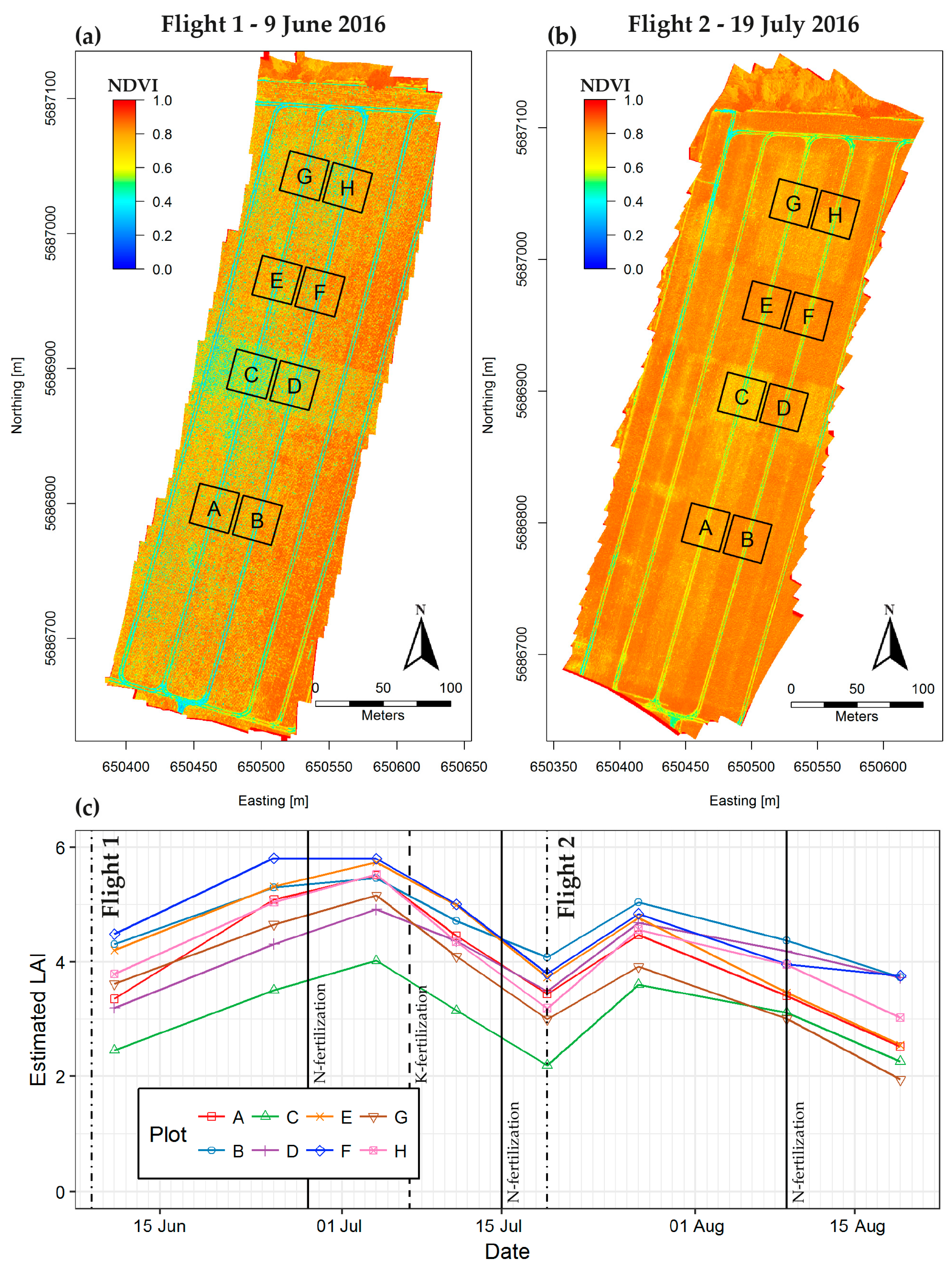
3.1. Crop Development
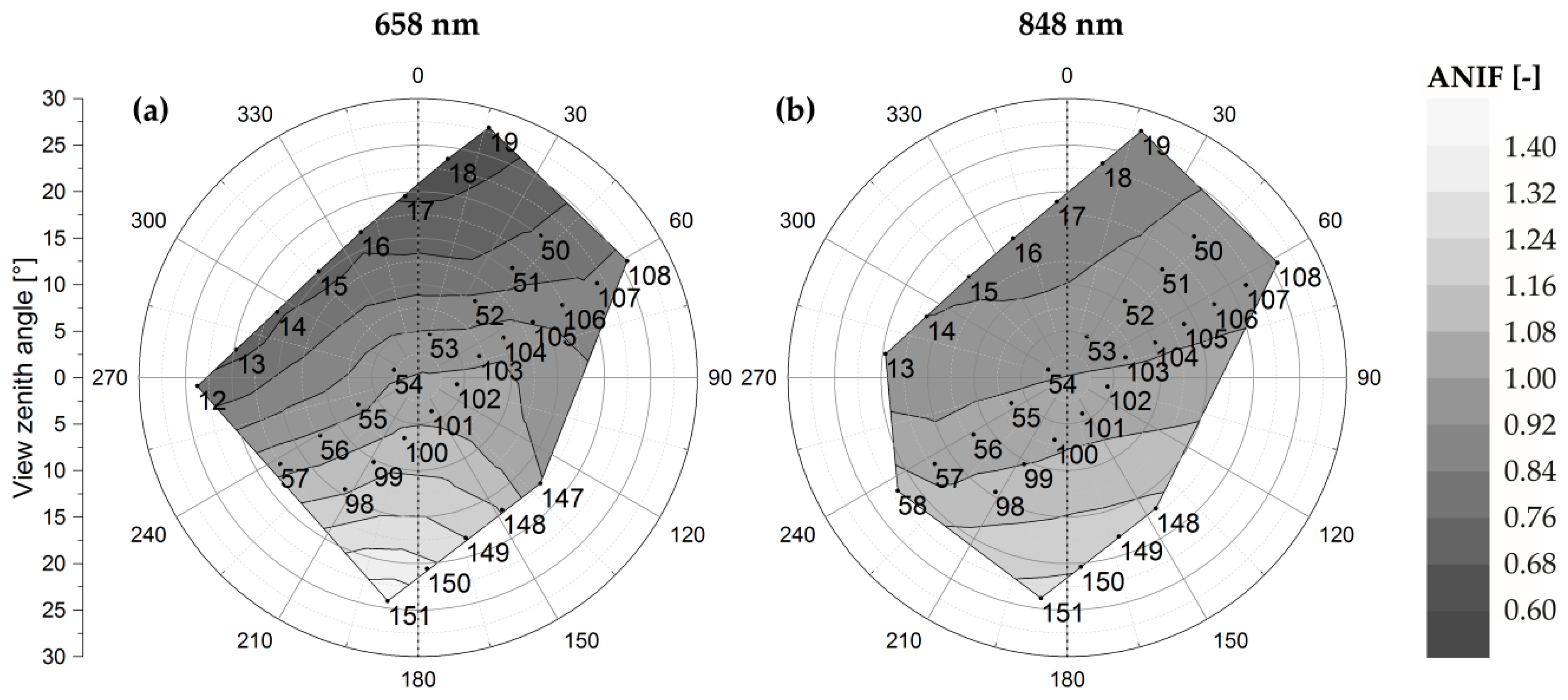
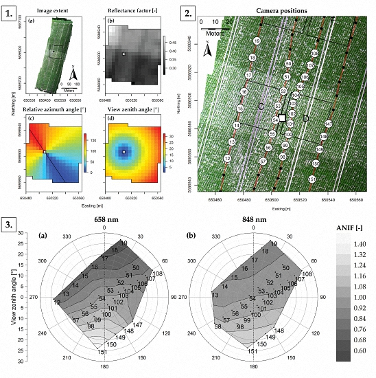
3.2. View Angle Coverage
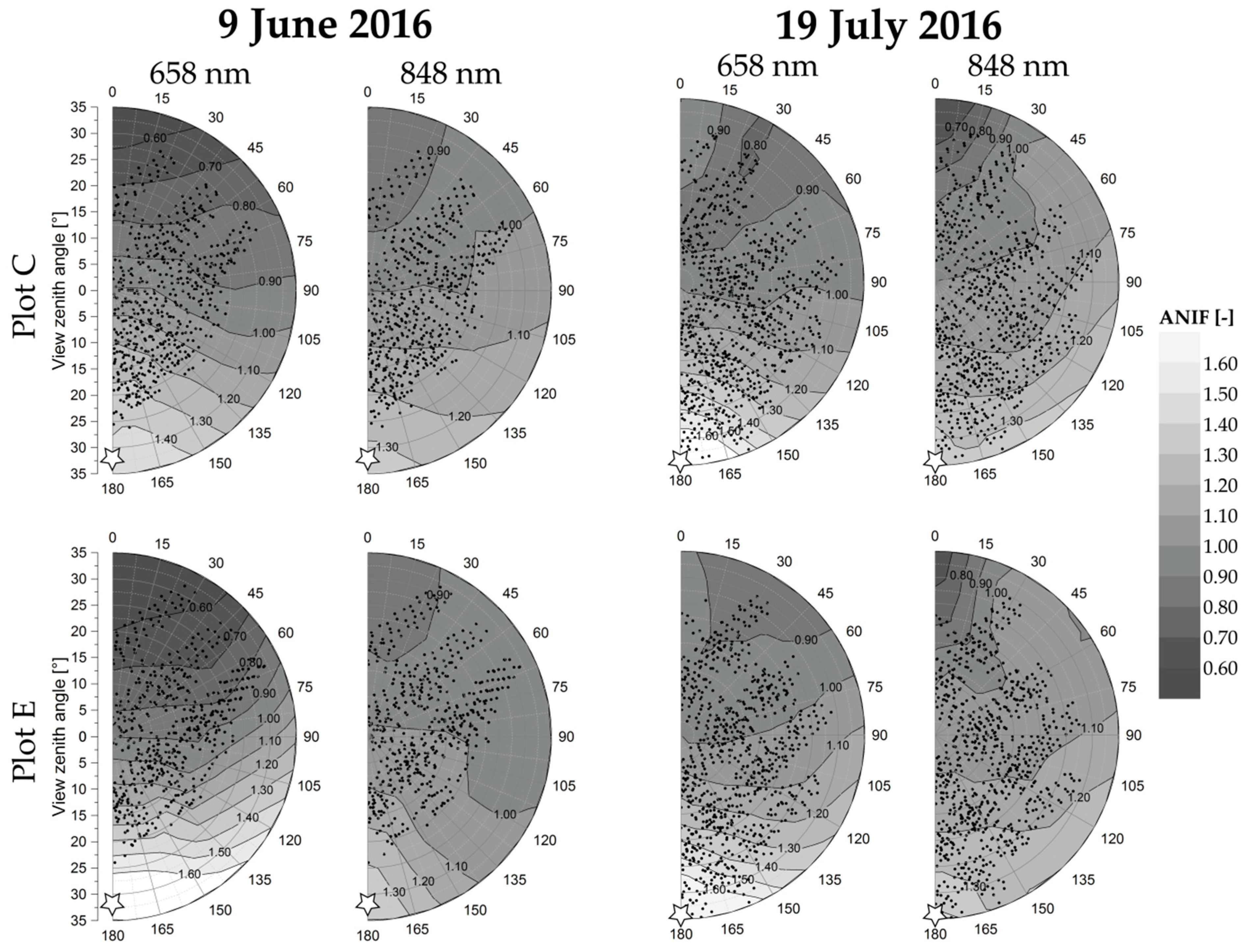
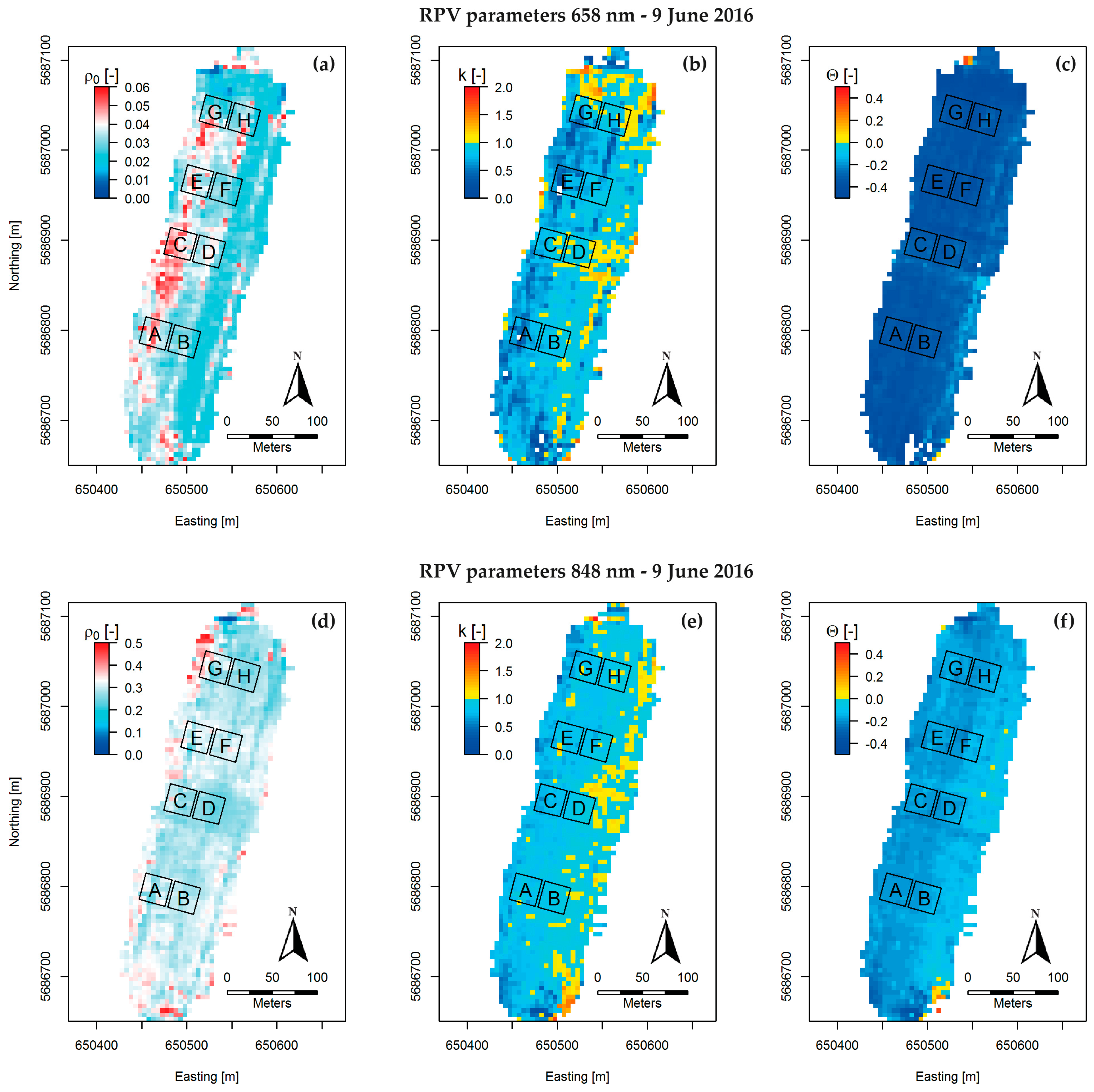
3.3. Anisotropy Maps
3.4. Plot Statistics
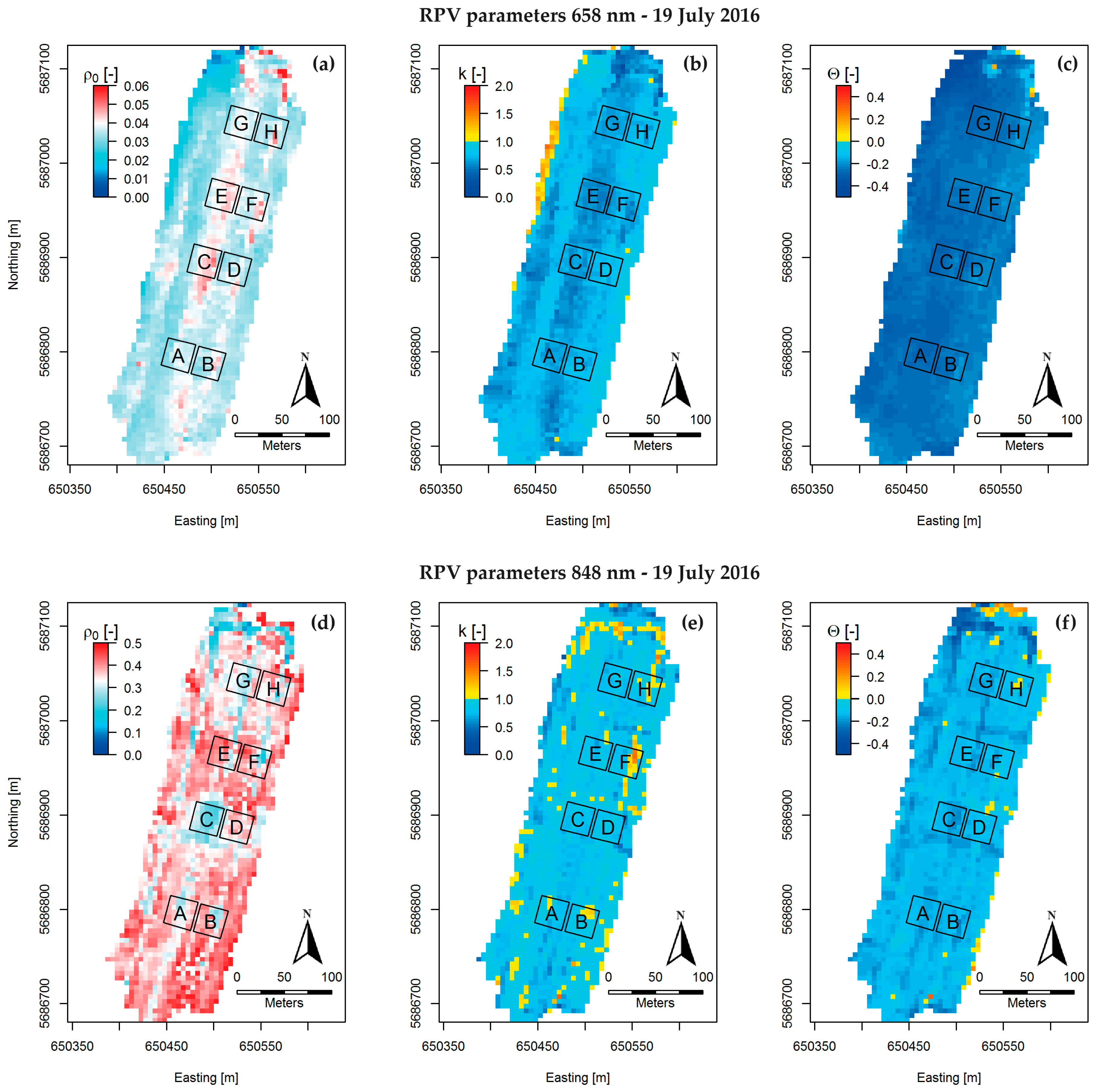
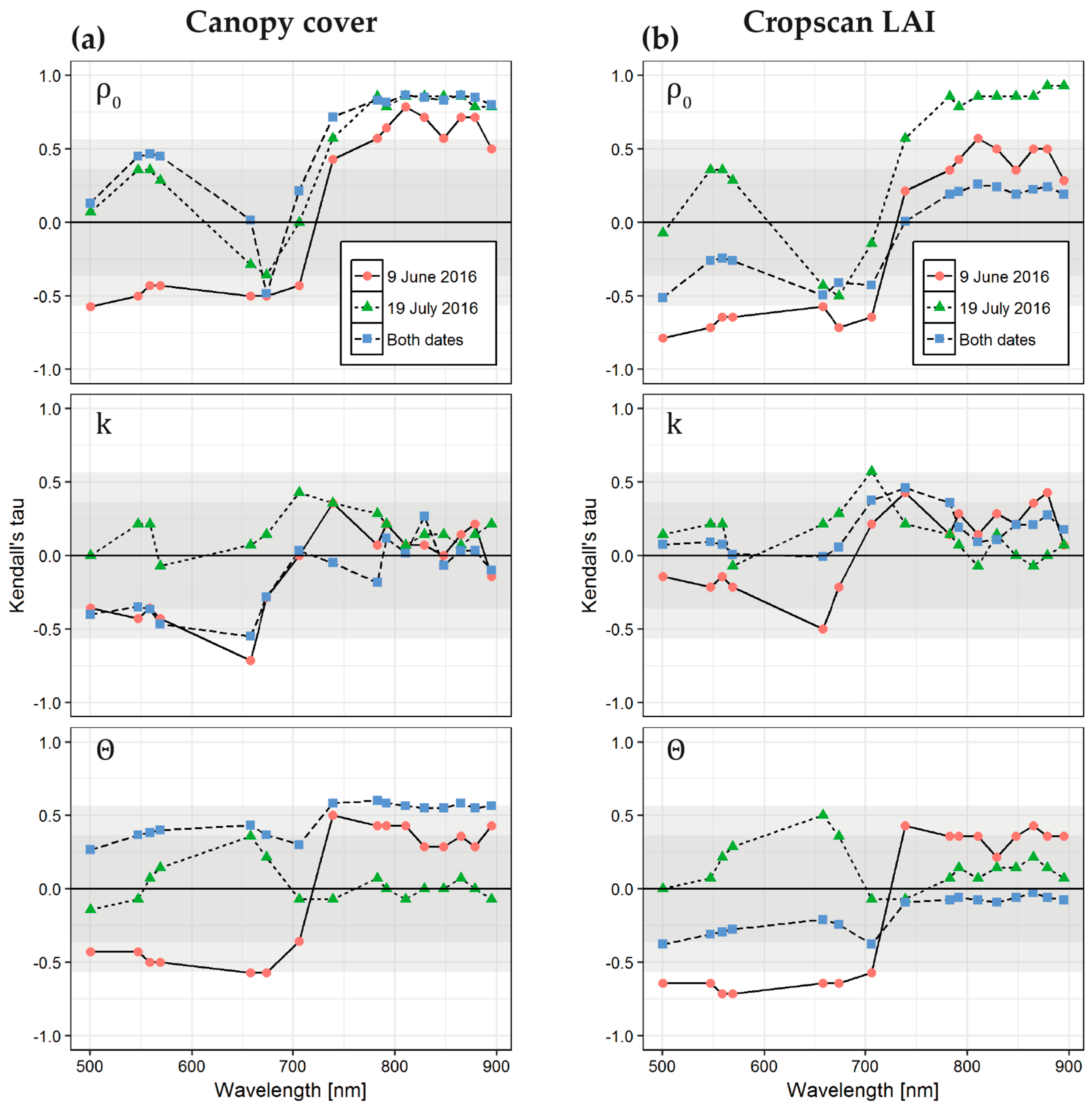
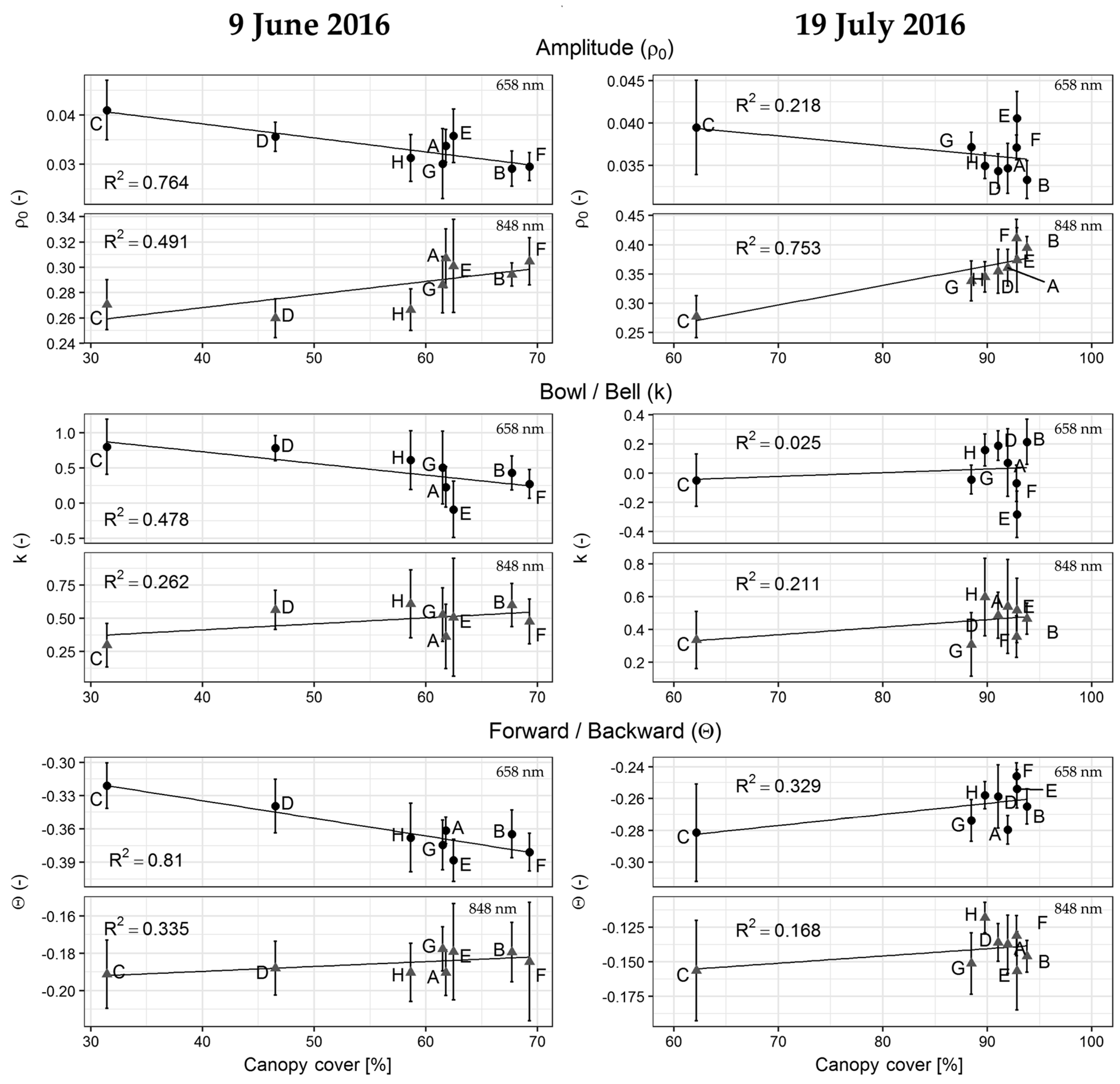
3.5. RPV Parameters vs. Canopy Cover and LAI
4. Discussion
5. Conclusions
Acknowledgments
Author Contributions
Conflicts of Interest
References
- Schaepman-Strub, G.; Schaepman, M.E.; Painter, T.H.; Dangel, S.; Martonchik, J.V. Reflectance quantities in optical remote sensing-definitions and case studies. Remote Sens. Environ. 2006, 103, 27–42. [Google Scholar] [CrossRef]
- Kimes, D.S. Dynamics of directional reflectance factor distributions for vegetation canopies. Appl. Opt. 1983, 22, 1364–1372. [Google Scholar] [CrossRef] [PubMed]
- Sandmeier, S.; Müller, C.; Hosgood, B.; Andreoli, G. Physical mechanisms in hyperspectral BRDF data of grass and watercress. Remote Sens. Environ. 1998, 66, 222–233. [Google Scholar] [CrossRef]
- Sun, T.; Fang, H.; Liu, W.; Ye, Y. Impact of water background on canopy reflectance anisotropy of a paddy rice field from multi-angle measurements. Agric. For. Meteorol. 2017, 233, 143–152. [Google Scholar] [CrossRef]
- Hill, M.J.; Averill, C.; Jiao, Z.; Schaaf, C.B.; Armston, J.D. Relationship of MISR RPV parameters and MODIS BRDF shape indicators to surface vegetation patterns in an australian tropical savanna. Can. J. Remote Sens. 2008, 34 (Suppl. S2), S247–S267. [Google Scholar] [CrossRef]
- Lavergne, T.; Kaminski, T.; Pinty, B.; Taberner, M.; Gobron, N.; Verstraete, M.M.; Vossbeck, M.; Widlowski, J.L.; Giering, R. Application to MISR land products of an RPV model inversion package using adjoint and hessian codes. Remote Sens. Environ. 2007, 107, 362–375. [Google Scholar] [CrossRef]
- Widlowski, J.L.; Pinty, B.; Gobron, N.; Verstraete, M.M.; Diner, D.J.; Davis, A.B. Canopy structure parameters derived from multi-angular remote sensing data for terrestrial carbon studies. Clim. Chang. 2004, 67, 403–415. [Google Scholar] [CrossRef]
- Bousquet, L.; Lachérade, S.; Jacquemoud, S.; Moya, I. Leaf BRDF measurements and model for specular and diffuse components differentiation. Remote Sens. Environ. 2005, 98, 201–211. [Google Scholar] [CrossRef]
- Huang, W.; Niu, Z.; Wang, J.; Liu, L.; Zhao, C.; Liu, Q. Identifying crop leaf angle distribution based on two-temporal and bidirectional canopy reflectance. IEEE Trans. Geosci. Remote Sens. 2006, 44, 3601–3608. [Google Scholar] [CrossRef]
- Feingersh, T.; Ben-Dor, E.; Filin, S. Correction of reflectance anisotropy: A multi-sensor approach. Int. J. Remote Sens. 2010, 31, 49–74. [Google Scholar] [CrossRef]
- Roujean, J.L.; Leroy, M.; Deschamps, P.Y. A bidirectional reflectance model of the earth’s surface for the correction of remote sensing data. J. Geophys. Res. 1992, 97, 20455–20468. [Google Scholar] [CrossRef]
- Schaaf, C.B.; Gao, F.; Strahler, A.H.; Lucht, W.; Li, X.; Tsang, T.; Strugnell, N.C.; Zhang, X.; Jin, Y.; Muller, J.P.; et al. First operational BRDF, albedo nadir reflectance products from modis. Remote Sens. Environ. 2002, 83, 135–148. [Google Scholar] [CrossRef]
- De Colstoun, E.C.B.; Walthall, C.L. Improving global scale land cover classifications with multi-directional polder data and a decision tree classifier. Remote Sens. Environ. 2006, 100, 474–485. [Google Scholar] [CrossRef]
- Duca, R.; Del Frate, F. Hyperspectral and multiangle chris-proba images for the generation of land cover maps. IEEE Trans. Geosci. Remote Sens. 2008, 46, 2857–2866. [Google Scholar] [CrossRef]
- Koukal, T.; Atzberger, C.; Schneider, W. Evaluation of semi-empirical BRDF models inverted against multi-angle data from a digital airborne frame camera for enhancing forest type classification. Remote Sens. Environ. 2014, 151, 27–43. [Google Scholar] [CrossRef]
- Su, L.; Huang, Y.; Chopping, M.J.; Rango, A.; Martonchik, J.V. An empirical study on the utility of brdf model parameters and topographic parameters for mapping vegetation in a semi-arid region with misr imagery. Int. J. Remote Sens. 2009, 30, 3463–3483. [Google Scholar] [CrossRef]
- Kneubühler, M.; Koetz, B.; Huber, S.; Schaepman, M.E.; Zimmermann, N.E. Space-based spectrodirectional measurements for the improved estimation of ecosystem variables. Can. J. Remote Sens. 2008, 34, 192–205. [Google Scholar]
- Wang, L.; Dong, T.; Zhang, G.; Niu, Z. LAI retrieval using PROSAIL model and optimal angle combination of multi-angular data in wheat. IEEE J. Sel. Top. Appl. Earth Obs. Remote Sens. 2013, 6, 1730–1736. [Google Scholar] [CrossRef]
- Wang, Y.; Li, G.; Ding, J.; Guo, Z.; Tang, S.; Wang, C.; Huang, Q.; Liu, R.; Chen, J.M. A combined glas and modis estimation of the global distribution of mean forest canopy height. Remote Sens. Environ. 2016, 174, 24–43. [Google Scholar] [CrossRef]
- Chen, J.M.; Menges, C.H.; Leblanc, S.G. Global mapping of foliage clumping index using multi-angular satellite data. Remote Sens. Environ. 2005, 97, 447–457. [Google Scholar] [CrossRef]
- He, L.; Chen, J.M.; Pisek, J.; Schaaf, C.B.; Strahler, A.H. Global clumping index map derived from the modis BRDF product. Remote Sens. Environ. 2012, 119, 118–130. [Google Scholar] [CrossRef]
- Biliouris, D.; Verstraeten, W.W.; Dutré, P.; Van Aardt, J.A.N.; Muys, B.; Coppin, P. A compact laboratory spectro-goniometer (CLabSpeG) to assess the BRDF of materials. Presentation, calibration and implementation on Fagus sylvatica L. leaves. Sensors 2007, 7, 1846–1870. [Google Scholar] [CrossRef]
- Roosjen, P.P.J.; Clevers, J.G.P.W.; Bartholomeus, H.M.; Schaepman, M.E.; Schaepman-Strub, G.; Jalink, H.; van der Schoor, R.; de Jong, A. A laboratory goniometer system for measuring reflectance and emittance anisotropy. Sensors 2012, 12, 17358–17371. [Google Scholar] [CrossRef] [PubMed]
- Bachmann, C.M.; Abelev, A.; Montes, M.J.; Philpot, W.; Gray, D.; Doctor, K.Z.; Fusina, R.A.; Mattis, G.; Chen, W.; Noble, S.D.; et al. Flexible field goniometer system: The goniometer for outdoor portable hyperspectral earth reflectance. J. Appl. Remote Sens. 2016, 10, 036012. [Google Scholar] [CrossRef]
- Coburn, C.A.; Peddle, D.R. A low-cost field and laboratory goniometer system for estimating hyperspectral bidirectional reflectance. Can. J. Remote Sens. 2006, 32, 244–253. [Google Scholar] [CrossRef]
- Deering, D.W.; Leone, P. A sphere-scanning radiometer for rapid directional measurements of sky and ground radiance. Remote Sens. Environ. 1986, 19, 1–24. [Google Scholar] [CrossRef]
- Painter, T.H.; Paden, B.; Dozier, J. Automated spectro-goniometer: A spherical robot for the field measurement of the directional reflectance of snow. Rev. Sci. Instrum. 2003, 74, 5179–5188. [Google Scholar] [CrossRef]
- Sandmeier, S.R.; Itten, K.I. A field goniometer system (FIGOS) for acquisition of hyperspectral BRDF data. IEEE Trans. Geosci. Remote Sens. 1999, 37, 978–986. [Google Scholar] [CrossRef]
- Suomalainen, J.; Hakala, T.; Peltoniemi, J.; Puttonen, E. Polarised multiangular reflectance measurements using the finnish geodetic institute field goniospectrometer. Sensors 2009, 9, 3891–3907. [Google Scholar] [CrossRef] [PubMed]
- Milton, E.J.; Schaepman, M.E.; Anderson, K.; Kneubühler, M.; Fox, N. Progress in field spectroscopy. Remote Sens. Environ. 2009, 113, S92–S109. [Google Scholar] [CrossRef]
- Painter, T.H.; Dozier, J. Measurements of the hemispherical-directional reflectance of snow at fine spectral and angular resolution. J. Geophys. Res. Atmos. 2004, 109, 1–21. [Google Scholar] [CrossRef]
- Peltoniemi, J.I.; Kaasalainen, S.; Näränen, J.; Matikainen, L.; Piironen, J. Measurement of directional and spectral signatures of light reflectance by snow. IEEE Trans. Geosci. Remote Sens. 2005, 43, 2294–2304. [Google Scholar] [CrossRef]
- Miller, I.; Forster, B.C.; Laffan, S.W.; Brander, R.W. Bidirectional reflectance of coral growth-forms. Int. J. Remote Sens. 2016, 37, 1553–1567. [Google Scholar] [CrossRef]
- Burkart, A.; Aasen, H.; Alonso, L.; Menz, G.; Bareth, G.; Rascher, U. Angular dependency of hyperspectral measurements over wheat characterized by a novel UAV based goniometer. Remote Sens. 2015, 7, 725–746. [Google Scholar] [CrossRef]
- Grenzdörffer, G.J.; Niemeyer, F. UAV based BRDF-measurements of agricultural surfaces with pfiffikus. Int. Arch. Photogramm. Remote Sens. Spat. Inf. Sci. 2011, 38, 229–234. [Google Scholar] [CrossRef]
- Roosjen, P.P.J.; Suomalainen, J.M.; Bartholomeus, H.M.; Clevers, J.G.P.W. Hyperspectral reflectance anisotropy measurements using a pushbroom spectrometer on an unmanned aerial vehicle-results for barley, winter wheat, and potato. Remote Sens. 2016, 8, 909. [Google Scholar] [CrossRef]
- Brede, B.; Suomalainen, J.; Bartholomeus, H.; Herold, M. Influence of solar zenith angle on the enhanced vegetation index of a guyanese rainforest. Remote Sens. Lett. 2015, 6, 972–981. [Google Scholar] [CrossRef]
- Colomina, I.; Molina, P. Unmanned aerial systems for photogrammetry and remote sensing: A review. ISPRS J. Photogramm. Remote Sens. 2014, 92, 79–97. [Google Scholar] [CrossRef]
- Hakala, T.; Suomalainen, J.; Peltoniemi, J.I. Acquisition of bidirectional reflectance factor dataset using a micro unmanned aerial vehicle and a consumer camera. Remote Sens. 2010, 2, 819–832. [Google Scholar] [CrossRef]
- Honkavaara, E.; Eskelinen, M.A.; Polonen, I.; Saari, H.; Ojanen, H.; Mannila, R.; Holmlund, C.; Hakala, T.; Litkey, P.; Rosnell, T.; et al. Remote sensing of 3-D geometry and surface moisture of a peat production area using hyperspectral frame cameras in visible to short-wave infrared spectral ranges onboard a small unmanned airborne vehicle (UAV). IEEE Trans. Geosci. Remote Sens. 2016, 54, 5440–5454. [Google Scholar] [CrossRef]
- Näsi, R.; Honkavaara, E.; Lyytikäinen-Saarenmaa, P.; Blomqvist, M.; Litkey, P.; Hakala, T.; Viljanen, N.; Kantola, T.; Tanhuanpää, T.; Holopainen, M. Using UAV-based photogrammetry and hyperspectral imaging for mapping bark beetle damage at tree-level. Remote Sens. 2015, 7, 15467–15493. [Google Scholar] [CrossRef]
- Rahman, H.; Pinty, B.; Verstraete, M.M. Coupled surface-atmosphere reflectance (CSAR) model 2. Semiempirical surface model usable with NOAA advanced very high resolution radiometer data. J. Geophys. Res. 1993, 98, 20791–20801. [Google Scholar] [CrossRef]
- Stoorvogel, J.J.; Kooistra, L.; Bouma, J. Managing soil variability at different spatial scales as a basis for precision agriculture. In Soil-Specific Farming: Precision Agriculture; CRC Press: Boca Raton, FL, USA, 2015; pp. 37–72. [Google Scholar]
- Clevers, J.G.P.W. Application of a weighted infrared-red vegetation index for estimating leaf area index by correcting for soil moisture. Remote Sens. Environ. 1989, 29, 25–37. [Google Scholar] [CrossRef]
- Kooistra, L.; Clevers, J.G.P.W. Estimating potato leaf chlorophyll content using ratio vegetation indices. Remote Sens. Lett. 2016, 7, 611–620. [Google Scholar] [CrossRef]
- Drusch, M.; Del Bello, U.; Carlier, S.; Colin, O.; Fernandez, V.; Gascon, F.; Hoersch, B.; Isola, C.; Laberinti, P.; Martimort, P.; et al. Sentinel-2: Esa’s optical high-resolution mission for gmes operational services. Remote Sens. Environ. 2012, 120, 25–36. [Google Scholar] [CrossRef]
- Rasmussen, J.; Ntakos, G.; Nielsen, J.; Svensgaard, J.; Poulsen, R.N.; Christensen, S. Are vegetation indices derived from consumer-grade cameras mounted on UAVs sufficiently reliable for assessing experimental plots? Eur. J. Agron. 2016, 74, 75–92. [Google Scholar] [CrossRef]
- Honkavaara, E.; Saari, H.; Kaivosoja, J.; Pölönen, I.; Hakala, T.; Litkey, P.; Mäkynen, J.; Pesonen, L. Processing and assessment of spectrometric, stereoscopic imagery collected using a lightweight UAV spectral camera for precision agriculture. Remote Sens. 2013, 5, 5006–5039. [Google Scholar] [CrossRef]
- Biliouris, D.; van der Zande, D.; Verstraeten, W.W.; Stuckens, J.; Muys, B.; Dutré, P.; Coppin, P. RPV model parameters based on hyperspectral bidirectional reflectance measurements of Fagus sylvatica L. leaves. Remote Sens. 2009, 1, 92–106. [Google Scholar] [CrossRef]
- Roosjen, P.P.J.; Bartholomeus, H.M.; Clevers, J.G.P.W. Effects of soil moisture content on reflectance anisotropy laboratory goniometer measurements and RPV model inversions. Remote Sens. Environ. 2015, 170, 229–238. [Google Scholar] [CrossRef]
- Maignan, F.; Bréon, F.M.; Lacaze, R. Bidirectional reflectance of earth targets: Evaluation of analytical models using a large set of spaceborne measurements with emphasis on the hot spot. Remote Sens. Environ. 2004, 90, 210–220. [Google Scholar] [CrossRef]
- Obidiegwu, J.E.; Bryan, G.J.; Jones, H.G.; Prashar, A. Coping with drought: Stress and adaptive responses in potato and perspectives for improvement. Front. Plant Sci. 2015, 6, 1–23. [Google Scholar] [CrossRef] [PubMed]
- Schlapfer, D.; Richter, R.; Feingersh, T. Operational BRDF effects correction for wide-field-of-view optical scanners (BREFCOR). IEEE Trans. Geosci. Remote Sens. 2015, 53, 1855–1864. [Google Scholar] [CrossRef]
- Verger, A.; Vigneau, N.; Chéron, C.; Gilliot, J.M.; Comar, A.; Baret, F. Green area index from an unmanned aerial system over wheat and rapeseed crops. Remote Sens. Environ. 2014, 152, 654–664. [Google Scholar] [CrossRef]
- Honkavaara, E.; Hakala, T.; Nevalainen, O.; Viljanen, N.; Rosnell, T.; Khoramshahi, E.; Näsi, R.; Oliveira, R.; Tommaselli, A. Geometric and reflectance signature characterization of complex canopies using hyperspectral stereoscopic images from uav and terrestrial platforms. In International Archives of the Photogrammetry, Remote Sensing and Spatial Information Sciences; ISPRS Archives: Prague, Czech Republic, 2016; pp. 77–82. [Google Scholar]
- Verrelst, J.; Romijn, E.; Kooistra, L. Mapping vegetation density in a heterogeneous river floodplain ecosystem using pointable CHRIS/PROBA data. Remote Sens. 2012, 4, 2866–2889. [Google Scholar] [CrossRef]
- Jacquemoud, S.; Verhoef, W.; Baret, F.; Bacour, C.; Zarco-Tejada, P.J.; Asner, G.P.; François, C.; Ustin, S.L. PROSPECT + SALL models: A review of use for vegetation characterization. Remote Sens. Environ. 2009, 113 (Suppl. 1), S56–S66. [Google Scholar] [CrossRef]


| Plot | Initial Fertilization | Additional Fertilization | |
|---|---|---|---|
| Before Planting (kg N/ha) | 28 June 2016 (kg N/ha) | 15 July 2016 (kg N/ha) | |
| A | 40 | 0 | 0 |
| B | 40 | 42 | 30 |
| C | 0 | 0 | 0 |
| D | 0 | 140 | 30 |
| E | 70 | 0 | 0 |
| F | 70 | 0 | 49 |
| G | 25 | 0 | 0 |
| H | 25 | 84 | 38 |
| Flight # | Date | Start Time | End Time | SAA (°) | SZA (°) |
|---|---|---|---|---|---|
| 1 | 9 June 2016 | 12:18 | 12:25 | 144–147 | 32–32 |
| 2 | 19 July 2016 | 12:29 | 12:37 | 147–150 | 34–33 |
| Band | Center Wavelength (nm) | FWHM (nm) |
|---|---|---|
| 1 | 500.2 | 14.8 |
| 2 | 547.0 | 13.2 |
| 3 | 558.8 | 13.0 |
| 4 | 568.8 | 12.9 |
| 5 | 657.6 | 13.0 |
| 6 | 673.6 | 13.2 |
| 7 | 705.8 | 13.1 |
| 8 | 739.0 | 19.4 |
| 9 | 782.8 | 18.5 |
| 10 | 791.6 | 18.4 |
| 11 | 810.3 | 18.1 |
| 12 | 829.0 | 17.8 |
| 13 | 847.8 | 17.6 |
| 14 | 864.7 | 17.4 |
| 15 | 878.7 | 17.3 |
| 16 | 894.7 | 17.1 |
| Plot | 9 June 2016 | 19 July 2016 | ||
|---|---|---|---|---|
| Cropscan (LAI) | Canopy Cover (%) | Cropscan (LAI) | Canopy Cover (%) | |
| A | 3.35 | 61.8 | 3.43 | 91.9 |
| B | 4.31 | 67.7 | 4.08 | 93.8 |
| C | 2.45 | 31.5 | 2.19 | 62.1 |
| D | 3.20 | 46.5 | 3.49 | 91.0 |
| E | 4.20 | 62.5 | 3.73 | 92.8 |
| F | 4.48 | 69.3 | 3.79 | 92.8 |
| G | 3.62 | 61.5 | 2.99 | 88.5 |
| H | 3.79 | 58.7 | 3.19 | 89.8 |
© 2017 by the authors. Licensee MDPI, Basel, Switzerland. This article is an open access article distributed under the terms and conditions of the Creative Commons Attribution (CC BY) license (http://creativecommons.org/licenses/by/4.0/).
Share and Cite
Roosjen, P.P.J.; Suomalainen, J.M.; Bartholomeus, H.M.; Kooistra, L.; Clevers, J.G.P.W. Mapping Reflectance Anisotropy of a Potato Canopy Using Aerial Images Acquired with an Unmanned Aerial Vehicle. Remote Sens. 2017, 9, 417. https://doi.org/10.3390/rs9050417
Roosjen PPJ, Suomalainen JM, Bartholomeus HM, Kooistra L, Clevers JGPW. Mapping Reflectance Anisotropy of a Potato Canopy Using Aerial Images Acquired with an Unmanned Aerial Vehicle. Remote Sensing. 2017; 9(5):417. https://doi.org/10.3390/rs9050417
Chicago/Turabian StyleRoosjen, Peter P. J., Juha M. Suomalainen, Harm M. Bartholomeus, Lammert Kooistra, and Jan G. P. W. Clevers. 2017. "Mapping Reflectance Anisotropy of a Potato Canopy Using Aerial Images Acquired with an Unmanned Aerial Vehicle" Remote Sensing 9, no. 5: 417. https://doi.org/10.3390/rs9050417
APA StyleRoosjen, P. P. J., Suomalainen, J. M., Bartholomeus, H. M., Kooistra, L., & Clevers, J. G. P. W. (2017). Mapping Reflectance Anisotropy of a Potato Canopy Using Aerial Images Acquired with an Unmanned Aerial Vehicle. Remote Sensing, 9(5), 417. https://doi.org/10.3390/rs9050417