Abstract
Synoptic monitoring of estuaries, some of the most bio-diverse and productive environments on Earth, is essential to study small-scale water dynamics and its role on spatiotemporal variation in water quality important to indigenous marine species and surrounding human settlements. We present a detailed study of turbidity, an optical index of water quality, in Apalachicola Bay, Florida (USA) using historical in situ measurements and Landsat 5 TM data archive acquired from 2004 to 2011. Data mining techniques such as time-series decomposition, principal component analysis, and classification tree-based models were utilized to decipher time-series for examining variations in physical forcings, and their effects on diurnal and seasonal variability in turbidity in Apalachicola Bay. Statistical analysis showed that the bay is highly dynamic in nature, both diurnally and seasonally, and its water quality (e.g., turbidity) is largely driven by interactions of different physical forcings such as river discharge, wind speed, tides, and precipitation. River discharge and wind speed are the most influential forcings on the eastern side of river mouth, whereas all physical forcings were relatively important to the western side close to the major inlet, the West Pass. A bootstrap-optimized and atmospheric-corrected single-band empirical relationship (Turbidity (NTU) = 6568.23 × (Reflectance )1.95; R2 = 0.77 ± 0.06, range = 0.50–0.91, N = 50) is proposed with seasonal thresholds for its application in various seasons. The validation of this relationship yielded R2 = 0.70 ± 0.15 (range = −0.96–0.97; N = 38; RMSE = 7.78 ± 2.59 NTU; Bias (%) = −8.70 ± 11.48). Complex interactions of physical forcings and their effects on water dynamics have been discussed in detail using Landsat 5 TM-based turbidity maps during major events between 2004 and 2011. Promising results of the single-band turbidity algorithm with Landsat 8 OLI imagery suggest its potential for long-term monitoring of water turbidity in a shallow water estuary such as Apalachicola Bay.
Keywords:
Apalachicola Bay; Landsat; turbidity; bootstrapping; classification tree; PCA; turbidity maps 1. Introduction
Estuaries are economically important and bio-diverse zones located between terrestrial and marine environments. Highly dynamic physicochemical conditions, such as nutrient richness, steep light and salinity gradients, and highly variable water column stratification conditions, well-mixed water column, make these transition zones some of the most productive regions in the coastal ocean [1]. Apalachicola Bay, Florida (USA), is such an estuary that has experienced significant urbanization and population-stress due to its economic-importance, thus necessitating a regular and synoptic monitoring of the bay’s water quality [2,3]. Turbidity is an optical index of water quality that directly impacts light availability to the photosynthetic organisms (e.g., phytoplankton and submerged vegetation), and in many cases can be directly linked to the amounts of suspended particulate matter (SPM) [4,5,6,7]. High turbidity is commonly responsible for obscuring the vision of marine nekton, damaging early-stage larval development, affecting prey-predator interactions, and causing significant mortality of commercially-important species (e.g., oysters) [8,9]. Spatiotemporal monitoring of water turbidity can further provide useful information about SPM and its impact on marine biota [4,10,11], the distribution and transport of SPM-coupled pollutants [12], and on depositional/erosional events [13,14,15] in coastal and inland environments.
Conventional turbidity monitoring requires an extensive network of in situ observations that can be demanding in both time and cost. In addition, traditional in situ methods are limited by poor spatial and temporal coverage to resolve estuarine-scale processes. Alternatively, continuous measurement strategies (e.g., point locations with data-loggers) may resolve temporal variations in water turbidity at specified locations, yet fail to provide synoptic representations of water dynamics and bay-shelf exchanges. Turbidity is a measure of incoming light attenuation, mainly due to particle scattering [16], while, water-leaving radiance carries information about optically-active water constituents [17]. Hence, a successful linkage between these optical parameters is a key tool in obtaining synoptic views of estuarine-scale turbidity distribution—using remote sensing platforms (e.g., satellites). Numerous studies have reported effective ways to utilize satellites in monitoring turbidity and suspended particulate matter in inland and coastal waters [18,19,20,21,22,23,24]. However, it is important to remember that water turbidity is closely linked to the optical characteristics of particles (e.g., particle size, shape, and composition), rather than just mass-specific properties such as particle weight and concentration [25]. Hence, the direct comparisons of particles in suspension and turbidity are still critically needed in these dynamic environments where particle properties change rapidly.
In the past few decades, advances in satellite technology have opened new horizons for achieving efficient monitoring of water quality in coastal and inland waters [19,21,26,27,28]. The ocean color satellite sensors such as MODIS (Aqua and Terra), OCM-2, VIIRS, and GOCI provide temporal coverage of hours to days with coarse spatial resolution. Although the temporal coverage of these sensors may aid the study of short time-scale processes (e.g., hours to days), their coarser spatial resolution limits applications to estuarine-scale water dynamics and turbidity distribution. In contrast, Landsat 5 TM sensor provides fine resolution of ~30 m to study small estuaries (e.g., Apalachicola Bay), but is limited by a longer revisit time of 16 days and poor signal-to-noise ratio compared to its successors (e.g., ETM+ and OLI) and the ocean color satellites.
In this paper, we investigate turbidity climatology over an 8-year period (2004–2011) in Apalachicola Bay. The aim of this study was to examine seasonally-varying water dynamics and its effect on the bay’s turbidity distribution, and therefore, importance was given to the spatial resolution rather than temporal coverage of a satellite sensor. Using historical Landsat 5 TM imagery in conjunction with in situ point measurements, we propose a single-band empirical relationship for monitoring turbidity in Apalachicola Bay, Florida (USA). The performance of Landsat 5 TM—turbidity relationship was also evaluated on the recently launched Landsat 8 OLI imagery. A time-series of turbidity was then analyzed using advanced statistical techniques to investigate the effects of meteorological, hydrological, and astronomical forcing on the water turbidity in Apalachicola Bay. Using the Landsat-based turbidity maps and in situ observations, we examined spatial variability in the bay’s turbidity and water dynamics seasonally and during major hydrological and meteorological events, such as the Apalachicola River floods, passages of the cold fronts, and the hurricane landfall during our study period. Water quality monitoring strategy presented in this study supports the US Environmental Protection Agency’s (EPA) water quality standards under the Clean Water Act to protect human health and the environment.
2. Materials and Methods
2.1. Study Area
Apalachicola Bay is an elongated shallow (average depth = ~3 m) estuarine system located in the Florida’s Panhandle that covers an area of ~540 km2 (Figure 1) [29]. Apalachicola River, the largest river in Florida, is the main source of freshwater and nutrients in the bay [30]. The bay is bounded by four barrier islands (St. Vincent, St. George, St. Little George, and Dog), and exchanges water through three natural passes (Indian, West, and East) and one man-made pass (Sikes Cut). Apalachicola Bay is one the most productive estuarine systems in North America. For example, it is well-known for its oyster harvest that supplies ~90% of the oysters in Florida, and accounts for ~10% of nationwide oyster production [31]. However, environmental stresses such as salt-water intrusion [32], tropical storms [33], Deep Water Horizon oil spill [34], and droughts/floods [35,36] have negatively affected the bay’s commercial oyster industry. Historical sediment records showed a decrease in nutrient levels in Apalachicola Bay possibly due to the reduction in river discharge and rising sea-level [37]. The bay is located in a transition zone, where diurnal tides of the western Gulf change to semi-diurnal tides towards the Florida’s Panhandle [38,39]. It also experiences relatively shorter periods of strong winds during extreme weather events, such as cold fronts, storms, and hurricanes that can have large effects on the bay’s water quality [40,41].

Figure 1.
Apalachicola Bay, USA (white star in inset). In situ turbidity is observed near DB (Dry Bar) and CP (Cat Point) stations. White star represents a meteorological station maintained by Apalachicola National Estuarine Research Reserve (ANERR). Arrows represent various natural and man-made connections between the bay and the Gulf of Mexico.
2.2. Data Sources
A list of in situ and satellite measurements with their sources and purpose in this analysis is given in Table 1. Meteorological and hydrological data, such as wind speed, wind direction, river discharge, tidal height, and rainfall, were requested from various state and federal agencies. Water quality measurements, such as turbidity and salinity, were collected from the Apalachicola National Estuarine Research Reserve (ANERR)-maintained YSI-6600 series sondes (YSI Inc., Yellow Springs, OH, USA) positioned ~0.3 m above the bottom at two locations, Cat Point (CP) and Dry Bar (DB) (Figure 1). Three sets of clear-sky Landsat imagery with no sun-glint artifact were requested from USGS Landsat data archive that include 19 images of Landsat TM, ETM+ and OLI sensors for validating ENVI-FLAASH atmospheric correction, 57 images of Landsat TM sensor for developing turbidity algorithm and spatial analysis, and 17 images of Landsat OLI sensor for evaluating the performance of proposed algorithm on Landsat 8 OLI imagery.

Table 1.
A list of data that are used in 8-year turbidity analysis (2004 to 2011) in Apalachicola Bay.
2.3. Methods
2.3.1. Overview
The main aim of this study was to examine the effects of physical forcings (e.g., Apalachicola River, winds, precipitation, and tides) on water turbidity, and to investigate the possible use of Landsat sensors (e.g., Landsat 5 TM) to get synoptic views of estuarine water dynamics and turbidity distribution in Apalachicola Bay. Regular monitoring of water quality parameters using space-borne sensors generally requires two necessary steps: (1) to achieve reasonable estimates of water-leaving radiance by removing atmospheric contributions from a signal received at the top-of-atmosphere (TOA); and (2) to obtain a robust relationship between water quality (e.g., turbidity) and satellite-based optical parameters (e.g., remote sensing reflectance—Rrs and surface reflectance—ρ) [42]. Remote sensing over water is quite challenging mainly due to low contributions of water-leaving light, and strong influence of atmosphere (~90%) to light sensed at the TOA. Consequently, it is necessary to remove atmospheric signal prior to the usage of satellite data for ocean color applications [43]. Numerous methods have been proposed for the removal of the atmospheric contribution to get better estimation of water-leaving radiance [43,44,45,46,47,48]. The complexity associated with these schemes makes them time-intensive and unsuitable for day-to-day monitoring purposes. Freely available tools (e.g., SeaDAS (OBPG, NASA)) incorporate many of these schemes for satellite data processing, but these tools do not support the older Landsat 5 TM sensor data. This study used a commercially available ENVI-FLAASH® (Fast Line of sight Atmospheric Analysis of Spectral Hypercubes) atmospheric correction module to correct clear-sky Landsat 5 TM imagery acquired for the analysis. However, the validation of FLAASH results (e.g., surface reflectance) was a necessary step before algorithm development and analysis. Furthermore, this study mainly focused on the historical data, and in situ matchups for validation analysis were not available over the study area. To obtain confidence on FLAASH’s performance in moderately turbid coastal waters, the atmospheric-correction module was tested first near the only available AERONET-OC site in the Gulf of Mexico. Subsequently, Landsat 5 TM—turbidity relationships were analyzed for different seasons, and a robust general relationship was developed using statistical techniques for converting atmospheric-corrected Landsat imagery into the turbidity maps in Apalachicola Bay. A schematic diagram (Figure 2) illustrates the pathways to generate turbidity maps in the bay wherein, AERONET-FLAASH comparison is represented by Path 1 (dashed lines), while satellite and in situ data quality check/processing are shown by Path 2 and Path 3, respectively.
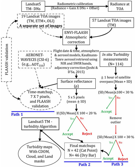
Figure 2.
A schematic diagram of processing pathways for developing an empirical relationship between in situ turbidity and atmospheric-corrected Landsat 5 TM red band (Band 3). Dashed lines represent processing units for AERONET—FLAASH validation on a separate set of 19 clear-sky images. DNs = Digital numbers, TM = Thematic mapper, ETM+ = Enhanced thematic mapper, OLI = Operational land imager, TOA = Top-of-the-atmosphere, and CDOM = Chromophoric Dissolved Organic Matter.
2.3.2. Landsat Image Processing
Raw at-sensor radiance images were corrected for the atmosphere using the ENVI-FLAASH® module (Exelis Visual Information Solutions, 2015). Radiometric-calibration was applied first to all of the raw images to convert at-sensor DNs (digital numbers) to at-sensor radiance values (LTOA) at each spectral band,
where C0, is the offset and C1 the gain coefficients of Landsat 5 TM for the corresponding band n. Surface-leaving radiance (Lu) conveys valuable information about the in-water constituents, but it contributes only about 10% to the LTOA. Major part of LTOA is contributed by the atmosphere (aerosols and gases), specular reflection of directly transmitted sunlight from the water surface (sun glint), direct reflected radiance from the water surface (sky light) and radiance reflected from whitecaps. The FLAASH module facilitates automated atmospheric correction with MODTRAN4 code over water using NIR (Band 4) and SWIR (Band 5) channels. The FLAASH processing methodology [49] is briefly described next. At sensor radiance is given by,
where, = surface reflectance of target pixels, = spatially averaged surface reflectance of surrounding region, A and B = coefficients that depend on atmospheric and geometric conditions, S = the spherical albedo of the atmosphere, = radiance that is received at the top-of-the-atmosphere (TOA), = radiance that is back-scattered by the atmosphere (aerosols, gases, and water molecules) to the sensor’s field of view. In Equation (2), includes radiance contributions from mainly 3 paths, (1) path radiance which is light scattered by the atmosphere (first term); (2) surface radiance which includes water-leaving radiance (Lw), part of sky light (Lsky1), and part of sun-glint (Lglint1) from that reflected from target pixels (second term); and (3) surface radiance that is diffusely transmitted into sensor, giving rise to “adjacency effect” (third term). It also includes part of skylight (Lsky2) and part of sun-glint (Lglint2) from the surrounding pixels.
Ln = C0n + C1n × DNn
In processing, FLAASH first utilizes MODTRAN4 radiative transfer model to calculate A, B, S and Latm by using manually provided image-based information such as viewing and solar angles (date and time of image acquisition), the mean surface elevation of the measurement (~705 km for Landsat 5 TM), model atmosphere (Mid-Latitude summer or Tropical based on in situ air temperature and month of image acquisition), and aerosol model (maritime-aerosol model). FLAASH includes a method for retrieving the aerosol amount and estimating a scene average visibility using an automated dark-pixel reflectance ratio method [50]. A dark-pixel is obtained by using an infrared wavelength (usually 2.1 μm; Landsat 5 TM Band 7) at which reflectance retrieval is generally insensitive to visibility. FLAASH then uses the Landsat bands 4 (NIR) and 7 (SWIR) with a nominal reflectance ratio (1 or 0.81) and a band 4 reflectance cutoff of 0.03. This assumes that the source of water reflectance in the infrared is spectrally flat or foam (white caps) with reflectance ratio 1 representing spectrally flat assumption whereas 0.81 is better suited for foam conditions (Moore, Voss, and Gordon, 2000). The visibility estimate is then combined with MODTRAN4 aerosol representation to describe the atmosphere. The values of A, B, S and Latm are also strongly dependent on the water vapor column amount, which is generally not well-known and may vary across the scene. Landsat sensor does not have the appropriate bands to perform water retrieval, so it is determined according to the standard water column amount for the selected atmospheric model which is then multiplied by an optional water column multiplier (e.g., Mid-Latitude summer—2.08 gcm−2 and Tropical—4.11 gcm−2 in our case).
Next, spatial averaging is implied by convolving radiance image of LTOA (Equation (2)) to find (at sensor) by using upward diffused transmission spatial point spread function that describes the relative contributions to the pixel radiance from points on the ground at different distances from the direct line of sight. is then obtained by neglecting contribution of surrounding pixels,
Once, , , A, B, and S are available, Equation (2) is solved for ρ (surface reflectance). It is important to note that adjacency correction partially removes sun-glint and skylight that is contributed by neighboring pixels; however, their exact values are unknown as they are removed during adjacency correction. Therefore, water surface reflectance (ρ) may have some effects of residual skylight and sun-glint. FLAASH-based image processing was used as described in Joshi and D’Sa (2015) [51]. After applying suitable quality-check criteria to remove the effects of outliers, average values of 5 × 5 and 7 × 7 pixels were calculated from the atmospherically-corrected Landsat images for turbidity algorithm and FLAASH—AERONET analysis, respectively, at each sampling site. We have used SeaDAS 7.2 (OBPG, NASA) to generate turbidity maps for further analysis (Figure 2).
2.3.3. FLAASH vs. AERONET
A separate analysis was performed to examine the validity of the FLAASH’s atmospheric correction. We used a different set of Landsat images (e.g., TM, ETM+, and OLI) collected over the AERONET WAVCIS CSI-6 site located to the south of Terrebonne Bay close to the Mississippi River delta (Figure 3). A validation analysis at CSI-6 can apply to Apalachicola Bay because of the similarity in turbidity conditions of the bay and the relatively low influence from the Mississippi-Atchafalaya river system at CSI-6. Nineteen clear-sky Landsat images (100% clear-sky image with no sun glint) were acquired over the AERONET station between 2011 and 2014. They included five Landsat 5 TM images, eight Landsat 7 ETM+ images and six Landsat 8 OLI images.
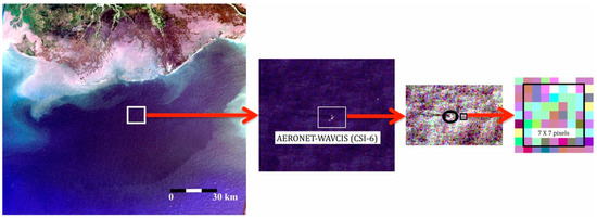
Figure 3.
AERONET WAVCIS (CSI-6) station, Gulf of Mexico (white box). A 7 × 7 box was chosen to the right of AERONET site rather than centered at the site to avoid noise from the station itself (black box).
The validity of FLAASH-corrected satellite observations was evaluated using two approaches, namely, (1) comparing the aerosol optical thickness (AOT); and (2) relating water-leaving radiance (Lw) or normalized water-leaving reflectance ( obtained from the in situ and satellite measurements. The first approach used AOT obtained from in situ AERONET measurements and Landsat images. In situ AOT acquired just before and after the satellite overpass were averaged to keep comparison closer to satellite measurement. Since the in situ AERONET measurements do not provide AOT (550 nm), these were obtained by the interpolation of nearby wavelengths. Furthermore, FLAASH utilizes MODTRAN4 code (which is not freely available) to calculate AOT (550 nm) using image data and historical climatology, but it does not provide AOT as an output in atmospheric-correction procedure. However, FLAASH does provide horizontal visibility which can be approximately converted to AOT using Koschmieder’s equation [52],
The second approach compared normalized water-leaving reflectance obtained from in situ measurements and atmospheric-corrected Landsat imagery. AERONET uses water-leaving radiance , ozone optical thickness (, Rayleigh optical thickness ( and aerosol optical thickness ( to obtain normalized water-leaving radiance (. is then converted to by using the following equation,
where, F0 = Extraterrestrial solar irradiance (mWcm−2µm−1) [53]. Satellite-based water-leaving reflectance () was obtained from FLAASH-corrected imagery with 7 × 7 box centered near to the AERONET site (Figure 3), which is then converted to [54],
where, θ = solar zenith angle, M is related to scattering phase function of aerosol.
2.3.4. Statistical Analysis
Time-series decomposition, principal component analysis (PCA), and classification-tree based models were used to examine relative importance of meteorological (e.g., wind speed and wind direction), hydrological (e.g., river discharge and salinity), and astronomical (e.g., tidal height) factors on the historical trends of turbidity in Apalachicola Bay. Time-series decomposition was applied using a loess-based seasonal-trend decomposition procedure (STL) [55]. The STL decomposes time-series into seasonal, yearly trend, and remainder components to extract useful information about seasonal, inter-annual, and random variations from the original time-series (“STL” package in R). PCA was used to show the complexity of Apalachicola Bay; this is a powerful dimension reduction technique that reduces a large number of variables into a few orthogonally separated principal components. Principal component is a linear transformation of the variables into a lower dimensional space that retains the maximum amount of information about the original variables. We used R statistical analysis software with “prcomp” package for the PCA analysis. Likewise, the relationship between turbidity and physical forcings, for example, could be strongly non-linear and involve complex interactions that could not be explained by commonly-used statistical modeling approaches. Classification (categorical dependent variable) and regression (numerical dependent variable) trees are the modern statistical techniques for exploring and modeling such a complexity in data [56], and have been widely used in a variety of fields such as agriculture, coastal environment [51], and freshwater and marine ecology [57,58]. Trees explain the variation of a single dependent variable corresponding to one or more explanatory variables by splitting data recursively based on the most influential independent variable. At each node, model splits observations into two mutually-exclusive groups based on a threshold value of the most influential explanatory variable by keeping each group as homogenous as possible with a minimum residual sum of squares. We used R statistical analysis software with “CART” package for the tree-based analysis.
It is complex to derive a general relationship for the diversity of sub-habitats in estuarine systems with a small sample size. Furthermore, the regression relationships between dependent and independent variables changes completely if a different set of training data is drawn from the sample every time. Therefore, uncertainty analysis is necessary for the reasonable estimates of regression coefficients and a robust general relationship for the study area. A bootstrapping approach was used with 5000 simulations to get reasonable estimates of regression coefficients for the Landsat 5 TM—turbidity relationship, and to obtain the validation statistics (e.g., Bias and root mean squared error (RMSE)) [59,60]. The bootstrapping is a machine-learning technique that provides reasonable inferential statistics for population with random and repeated sample selection, especially when the sample size is limited. In regression analysis, algorithm development and validation require the data to be divided in training and testing sets (e.g., training data = 50; testing data = 38 total data = 88). In processing, the first bootstrap-run picks up a training set from the given sample to develop a relationship between dependent and independent variables. Then, it validates this relationship on remaining data (e.g., testing set), and provides statistical inferences for the prediction accuracy. Next, the second bootstrap runs on the new set of randomly selected training and testing data sets, and provides statistical parameters and inferences of regression and validation (e.g., slope, intercept, R2, Bias, and RMSE). If bootstrapping procedure is run for N times on the given sample size, it can provide good estimates of regression coefficients and validation accuracy for the population. Furthermore, the means of regression coefficients (e.g., slope and intercept) can be used as the reasonable estimates for developing a general regression model if their distributions are not highly skewed. In this analysis, 5000 bootstrap simulations (training data = 50 and testing data = 38) provided population distributions of regression estimates, inferential statistics, and validation accuracy for the Landsat 5 TM—turbidity relationship in Apalachicola Bay.
3. Results and Discussion
3.1. Satellite Assessment of Water Turbidity in Apalachicola Bay
3.1.1. Assessing the Performance of ENVI-FLAASH Based Atmospheric Correction
The FLAASH derived AOT550 showed a good correlation (R2 = 0.96, RMSE = 0.011, N = 19) to in situ AOT550 that indicated a reasonable retrieval of aerosol properties by MODTRAN4 code (Figure 4a). However, the uncertainty increased towards low visibility (or high AOT) conditions. The Koschmieder’s equation (Equation (4)) assumes the equality in vertical and horizontal extinction coefficients with no effects of vertical extinction profile on the AOT. However, vertical extinction coefficient may become larger than horizontal extinction coefficient in many cases (e.g., high aerosol concentration in the upper atmospheric layers, and temperature inversions). Furthermore, the conversion of AOT from horizontal visibility may cause large RMSE especially for the visibility <30 km [52]. FLAASH-corrected and in situ also showed a reasonable agreement between satellite and above-water measurements (R2 = 0.86; N = 24) (Figure 4b).
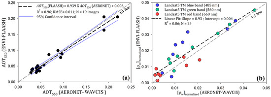
Figure 4.
An assessment of FLAASH-based atmospheric correction using in situ (a) aerosol optical thickness (AOT550), and (b) normalized water-leaving reflectance ([ρw]normalized) observed at AERONET-WAVCIS site in the northern Gulf of Mexico.
3.1.2. Band Selection
In principle, water turbidity is mainly a measure of the light scattered (back or side scattering of white or NIR light based on instrument design) from particles in suspension [16]. Therefore, it can be related to water-leaving light (e.g., Rrs and ρ) recorded by satellite sensor by assuming, (1) water column is homogenously mixed; and (2) surface water is spatially homogenous around the study area. Generally, estuaries, such as Apalachicola Bay, are highly productive due to their nutrient richness and light availability for the primary production [61]. Furthermore, they receive considerable amounts of sediments and dissolved organic matter (e.g., CDOM) from the river, its tributaries, and adjacent wetlands [62]. Also, physical forcings such as winds and tides make these shallow water systems optically complex due to water column mixing and bottom sediment re-suspension. Therefore, band selection for the turbidity algorithm is difficult especially in the estuarine environment where larger concentrations of major optical constituents do not co-vary.
Water turbidity can be mainly related to the presence of reflective particulate matter in a water column (e.g., non-algal particulate matter (NAP) and detritus). In natural waters, back-scattering spectra generally show a broad peak in blue-green region (e.g., 500–600 nm) that decreases towards blue and red regions possibly due to strong pigment absorption [63,64]. Additionally, the presence of CDOM further downgrades the water-leaving radiance at the blue and green wavelengths especially in CDOM-rich coastal waters such as Apalachicola Bay [65,66]. Therefore, these wavelengths are generally avoided for the remote sensing of suspended particles and turbidity especially in optically complex estuarine and inland waters. The CDOM and NAP absorptions decrease toward the red and NIR wavelength, and particle back-scattering becomes a major contributor to the surface reflectance except in chlorophyll-a absorption region (~670–680 nm). Several studies have demonstrated the successful application of red and NIR wavelengths to monitor water quality in coastal and estuarine environments [19,20,21,67,68,69]. Landsat 5 TM NIR band is broad (760–900 nm, band width = ~140 nm), and water absorption increases about an order of 4 from the red (~660 nm) to the NIR wavelength (~727.5 nm) [70]. Therefore, NIR band could be useful only in highly-turbid waters where particle back-scattering prevails over the water absorption, but it may not provide useful information about water clarity in low to moderately turbid waters [71]. This could be one of the reasons that NIR band showed relatively poor correlation (R2 = 0.55) with turbidity in Apalachicola Bay (Figure S1). On the other hand, red band could be useful as it has relatively narrower (630–690 nm) bandwidth with the dominance of back-scattering in the larger portion of bandwidth compared to the chlorophyll-a absorption, thus we have used surface reflectance (ρ) of Band 3 (red band) which was obtained from FLAASH-corrected Landsat imagery for algorithm development.
3.1.3. Landsat 5 TM-Turbidity Algorithm and Validation
Landsat 5 TM—turbidity relationships were evaluated separately for different seasons. Despite the influence of the chlorophyll absorption peak, the correlation between in situ turbidity and Landsat 5 TM reflectance (Band 3: 630–690 nm) was reasonably good in the spring (R2 = 0.79, N = 22), the fall (R2 = 0.89, N = 19), the winter (R2 = 0.76, N = 27) except in the summer (R2 = 0.50, N = 21) (Figure S2). The temporal variability in in situ measurements (± 1 h of satellite overpass) and pixel-to-pixel variability in surface reflectance (5 × 5 pixels centered close to in situ station) were relatively smaller in the spring, and the winter likely due to energetic mixing of water column by river discharge, and winds along with sustained-influence of these forces during the time of measurements. Both Cat Point and Dry Bar stations are located on the hard bottom substrate (with no vegetation) of productive oyster bars [72]. The large uncertainties in reflectance measurements in relatively clearer water scenarios indicated the possible contamination due to the variability in bottom reflectance at each pixel [73].
The bootstrap approach yielded reasonable statistics for turbidity algorithm (R2 = 0.77 ± 0.06, range = 0.50–0.91, N = 50), and its validation (R2 = 0.70 ± 0.15, range = -0.96 – 0.97, N = 38; RMSE = 7.78 ± 2.59 NTU) (Table S1; Figure S3). The regression coefficients for the mean RMSE (= 7.78 NTU) of simulations were considered as the reasonable estimates of slope and intercept for the following power-law relationship between turbidity and Landsat 5 TM red band (Figure 5a),

Figure 5.
(a) Turbidity algorithm using bootstrap estimations; (b) optimization of turbidity algorithm based on seasonal thresholds. Grey box represents data bounds for the general turbidity algorithm (black line), whereas colored boxes represents threshold bounds for different seasons (e.g., green for spring (ρmin = 0.01 and ρmax = 0.11), blue for winter (ρmin = 0.01 and ρmax = 0.08), yellow for fall (ρmin = 0.01 and ρmax = 0.07), and red for summer (ρmin = 0.01 and ρmax = 0.04).
3.1.4. An Optimization of the General Turbidity Algorithm Based on Seasonal Thresholds
Because the slope and range of the general turbidity algorithm are different than individual seasonal Landsat 5 TM—turbidity relationships, the usage of a general algorithm outside the ranges of individual relationships can cause erroneous estimates of turbidity. Therefore, using reflectance thresholds corresponding to different seasons further optimized the algorithm. The lower threshold (surface reflectance = 0.01), was kept the same for all the seasons whereas upper threshold, was selected where modeled seasonal relationships deviated significantly from the general turbidity algorithm as shown in Figure 5b (e.g., ρ = 0.11 for the spring, ρ = 0.08 for the winter, ρ = 0.07 for the fall, and ρ = 0.04 for the summer). Furthermore, any signature of strong bottom reflectance and skylight will result in very high reflectance at the surface. If signature is too high to cross the upper limits, the pixel will be masked out from the image and thus, erroneous pixels can be avoided in the analysis with the proposed thresholds.
3.2. Temporal Variations in Physical Forcings in Apalachicola Bay
3.2.1. Time-Series Analysis
Apalachicola Bay generally experienced elevated river flows in late winter and spring that gradually reduced to minimal flows towards the warm seasons (Figure 6a). Furthermore, a right-skewed frequency distribution of discharge (~558.21 ± 499.10 m3s−1) suggested that the bay usually experiences long periods of low-flow conditions and strong episodes of elevated river flow (Table S2; Figure S4). High river discharge were normally observed during the Apalachicola River flood events (e.g., March–April, 2005; 2008; 2009), and during passages of strong cold-frontal systems (e.g., January-February, 2010) (also see blue bars in Figure 6a). However, heavy precipitation and associated run-off in the lower ACF basin (Apalachicola-Chattahoochee-Flint) can also occasionally affected the freshwater inflow to the bay. Seasonally-decomposed precipitation revealed frequent occurrences of rainfall events in the summer and fall seasons (Figure 6b; Figure S5). The anomalously high river discharge and precipitation observed during winter and spring may have also been related to the weak and moderate El Niño events in 2004–2005 and 2009–2010, respectively [74,75].
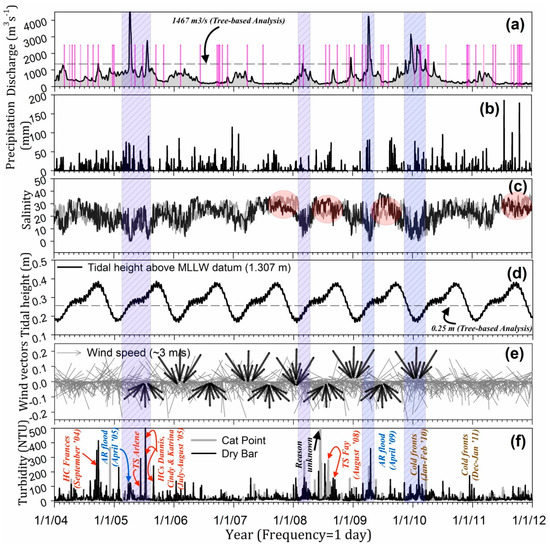
Figure 6.
Time-series of (a) Apalachicola River discharge (m3s−1); (b) precipitation (mm); (c) salinity, (d) tidal height (m); (e) wind speed (ms−1) and wind direction (°N); and (f) water turbidity (NTU) from 2004 to 2011. The gray-dashed line represents Cat Point (CP) station and black-solid line represents Dry Bar (DB) station in figures (c,f). Blue boxes illustrate the effects of high river flow conditions on salinity and water turbidity, e.g., salinity decreases and turbidity increases as river discharge increases. Red ellipses indicate the difference in salinity at two stations during the low-flow conditions. Black arrows illustrate wind direction during cold (downward) and warm (upward) seasons in general. Red bars in (a) represent Landsat 5 TM clear sky match-ups for turbidity algorithm and validation analysis during the study period. HC = Hurricane, TS = Tropical storm, AR = Apalachicola River.
Apalachicola Bay was relatively saline near to the freshwater sources in warm seasons, and was relatively fresher in winter and spring indicating seasonal-influence on the bay’s water quality (Figure 6c). Mean-daily salinity showed similar trends at Cat Point (CP) (21.69 ± 7.78) and Dry Bar (DB) (21.99 ± 7.45) stations, but they varied considerably in many instances possibly due to complex interactions of river, wind, precipitation, and tidal forcings during the study period (also see red ellipses in Figure 6c). The bay experiences a micro-tidal environment with tidal height of 0.28 m (± 0.06 m) above the mean lower low water datum (MLLW = 1.307 m). Diurnal tidal-range was relatively larger in spring and summer than in the fall and winter (Figure 6d). Furthermore, mean-daily tidal height showed a bimodal distribution with relatively higher tides in the summer and fall seasons, and relatively lower tides in winter. Although wind speed can vary significantly at shorter time intervals (e.g., minutes), the bay experienced low to moderate mean-daily wind speed (2.67 ± 1.06 ms−1) from 2004 to 2011 (Table S2). Wind vectors also showed yearly trends of strong northerly winds in winter and early spring, and relatively milder southerly winds in the summer and fall (Figure 6e).
A time-series of mean-daily turbidity showed irregular variations that could be attributed to complex interactions between the Apalachicola River plume, daily tidal cycles, precipitation, and erratic behavior of winds across the bay (Figure 6f). Mean turbidity at DB was relatively higher than at CP likely due to shallower depth and proximity to the major inlet at West Pass (Figure 1; Table S2). Large turbidity peaks were well-correlated with high-flow conditions in the Apalachicola River (blue boxes in Figure 6) and tropical storms [14,41]. A seasonally-decomposed turbidity suggested the difference in trends at two stations, e.g., Cat Point experienced turbid waters, whereas Dry Bay station remained less turbid in the summer (Figures S6 and S7). Despite the proximity to major river mouth, the observed differences in turbidity ranges could also be associated with complex mechanisms of plume dynamics in the bay (Table S2).
3.2.2. Principal Component Analysis
In Figure 7, each point represents physical state of the bay based on different physical variables, e.g., salinity, tidal height, river discharge etc. It is difficult to summarize the bay’s “conditions” with this many variables because some of them remain stable for most of the days (e.g., air temperature, while others vary more frequently during different days (e.g., wind speed). PCA generated new characteristics (e.g., principal components) with maximum possible variance in data for easier explanation (Figure 7). The PCA results showed that ~50% of the information (variance) contained in the data are retained by the first two principal components, which indicated that the variance in data can be explained by more than two principal components and in more than two dimension spaces. Principal component-1 (PC1) explained ~26% variance, and generally described the data based on seasonality (e.g., days in the winter and spring to the right) and in summer and fall to the left (Figure 7). Therefore, blue/green points in figure are the days of winter and spring when the bay experienced elevated river discharge, higher air pressures, more turbid waters at Dry Bar than at Cat Point, cold air temperatures, and became relatively fresher as compared to the summer and fall. Furthermore, a positive association of PC1 to the river discharge (~49%) and negative association with salinity (at Cat Point (~40%) and Dry Bar (~46%)) and tidal height (~40%), supported the time-series results which showed that the bay generally experienced moderate river discharge, low tidal heights, and low salinity environments in winter and spring, and vice versa.
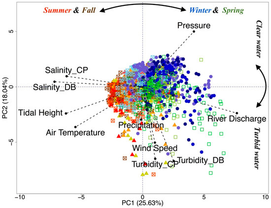
Figure 7.
Principal Component Analysis (N = 2377 days) on meteorological (wind speed, wind direction, and air temperature), hydrological (river discharge, precipitation, turbidity, and salinity), and astronomical (tidal height) variables in Apalachicola Bay. A color scheme and symbols are used to illustrate seasonality, e.g., blue color represent the winter (November to February), green square represent the spring (March to May), red triangle represents the summer (June to August), brown crossed-square boxes represent the fall (September & October). The shades of group color indicate months in each group, e.g., November—sky blue, January—Navy blue, July—orange, August—red. Turbidity_DB = Turbidity at Dry Bar, Turbidity_CP = Turbidity at Cat Point, Salinity_DB = Salinity at Dry Bar, and Salinity_CP = Salinity at Cat Point.
Conversely, principal component-2 (PC2) explained data generally based on water turbidity, whereby, less turbid days had positive scores on PC2 and more turbid days had negative scores on PC2. The PC2 was strongly related to wind speed and water turbidity at both locations indicating the importance of winds on diurnal variability in the bay’s turbidity. Loadings of river discharge were located closer to Dry Bar turbidity (Turbidity_DB), suggesting stronger influence of river discharge in the western part of bay (e.g., DB) than the eastern part (e.g., CP)—except during periods of strong westerly winds that could veer the river plume towards St. George Sound (Figure 1). Similarly, tides could affect more the turbidity at the CP compared to the DB station. As expected, high pressure and low temperatures were generally observed in the winter. Moreover, in many instances we observed positive correlations between high barometric pressures and river discharge, possibly due to wind-driven river flow during frontal passages. However, these interactions of frontal winds and river discharge, and their effects on turbidity, were not apparent in the PCA results. Overall, a small difference in first two principal components (25.63% and 18.04%, respectively) to explain variance in data indicated that various physical parameters strongly interact with each other, making Apalachicola Bay a complex estuarine system. Classification tree-based models were analyzed to further examine the relative importance of wind, tides, river discharge, and precipitation on the bay’s turbidity in the eastern and western regions of the bay.
3.2.3. Tree-Based Classification Models
Tree-based classification models showed relative importance of major physical forcings on the mean-daily turbidity at Cat Point (CP) and Dry Bar (DB) locations in Apalachicola Bay from 2004 to 2011. The mean turbidity at CP was 11 NTU (n = 2170 days). Similar to PCA, tidal height was the important factor at Cat Point that was used to classify data in two groups based on tidal influence, e.g., Node 2 (Tide < 0.25 m, turbidity = 8.3 NTU, n = 653 days), and Node 3 (Tide > 0.25 m, turbidity = 12 NTU, n = 1517 days) (Figure 8a). A tidal height threshold (0.25 m) separated data based on seasonal amplitudes, e.g., low tidal-height in winter and early spring, whereas high tidal-height in late spring, summer, and fall (Figure 6d). River discharge was a major contributor to the turbidity at Node 2. High-river flow conditions (RD > 1467 m3s−1) showed the largest increase in turbidity (Node 5, mean = 24 NTU, n = 33 days) that is likely to represent flood days (e.g., March–April, 2009; also see Figure 6a), and elevated river flow during frontal passages in winter months (e.g., December and January–2010; also see Figure 6a). Apalachicola River discharge is usually low in late spring, summer, and fall (Figure 6a and Figure 7), however the periods of moderate winds can likely lead to increase in water turbidity through water-column mixing or by veering of the river plume water towards the eastern part of the bay (Node 7, mean turbidity = 15 NTU, n = 682 days). Variable importance analysis showed that Apalachicola River discharge was the most influential forcing (~43%) associated with the largest variation in water turbidity, followed by wind speed (~32%) and tidal height (~19%). In contrast, precipitation had a least influence (~6%) on variability in turbidity to the eastern region of the bay (e.g., Cat Point).
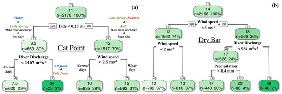
Figure 8.
Classification tree model for turbidity at (a) Cat Point; and (b) Dry Bar (right) in Apalachicola Bay from 2004 to 2011. Wind speed in ms−1, Apalachicola River discharge in m3s−1, tidal height in meter, and precipitation in millimeter.
At Dry Bar station, wind speed was the primary factor that explained variability in turbidity during the study period (Figure 8b). Mean water turbidity was generally ~50% higher during the strong winds (Node 3, Mean turbidity = 18, wind speed > 3 ms−1, n = 507) than weak winds (Node 2, Mean turbidity = 12 NTU, wind speed < 3 ms−1, n = 1453 days). In addition, periods of strong winds during high river flow and precipitation events showed significant increases in water turbidity (~142% and ~ 84% at Node-7 and Node-13, respectively) in comparison to the weak winds (Node 2) at the Dry Bar station. Variable importance analysis showed that wind speed (~36%) was the most important factor for daily turbidity variations that was followed by river discharge (~27%), precipitation (~23%), and tidal height (~14%) towards the western region of bay (e.g., Dry Bar).
3.2.4. Seasonal Turbidity Patterns in Apalachicola Bay
Apalachicola Bay’s turbidity ranges from 1 to 70 NTU during normal days [29]. According to US EPA’s (Environmental Protection Agency) water quality standards under the Clean Water Act (CWA), the bay’s water is classified as CLASS II water which is suitable for shellfish propagation and harvesting. Although turbidity classification of low, moderate and high levels varies with locations and importance of a water body, a turbidity reading of <10 NTU indicates fairly clean water for most of the lakes and rivers. Furthermore, the EPA has set a turbidity criterion of <29 NTU above background (5–10 NTU) as normal condition in the bay. Often however values can increase beyond 100 NTU especially during extreme events such as cold fronts, floods, and tropical storms. Based on this information, we classified turbidity levels as low (<10 NTU), moderate (10–50 NTU), and high (>50 NTU) in Apalachicola Bay.
Cross-year (2004–2011) seasonally mean turbidity maps showed distinct variations in spatial patterns of turbidity in Apalachicola Bay. Moderate turbidity (>10 NTU) was observed in central and east bays in the spring and the winter (Figure 9a,d). However, spatial extent of moderately turbid water was usually widespread and uniform in the spring indicating a strong influence of river discharge on the bay’s water turbidity in the wet season. In contrast, highly turbid water, mainly observed on shallow regions of the bay (e.g., EB, VC, and near barrier islands), was likely due to wind-supported sediment resuspension and river discharge in winter. Apalachicola Bay generally experiences low turbidity (<10 NTU) during low flow conditions (e.g., Figure 9b,c). Frequent periods of precipitation and run-off activities could be responsible for showing well-distributed turbid waters close to terrestrial sources as observed in summer. Nonetheless, the effects of bottom reflectance on the seasonal maps cannot be ignored (e.g., VS, CP, and DB) during low flow conditions (e.g., summer and fall). Bottom reflectance can be very pronounced in the fall when the bay lacks adequate supply of particulate material—via freshwater sources (e.g., rivers and run-off). However, short periods of wind-induced sediment resuspension could have resulted in moderate turbidity in central bay in the fall. St. George Sound (GS) remained relatively clear in all seasons possibly due to lack of freshwater sources and relatively deeper water column [72]. Seasonal turbidity maps also indicated that Apalachicola Bay can be generally classified as a low to moderately turbid estuary.
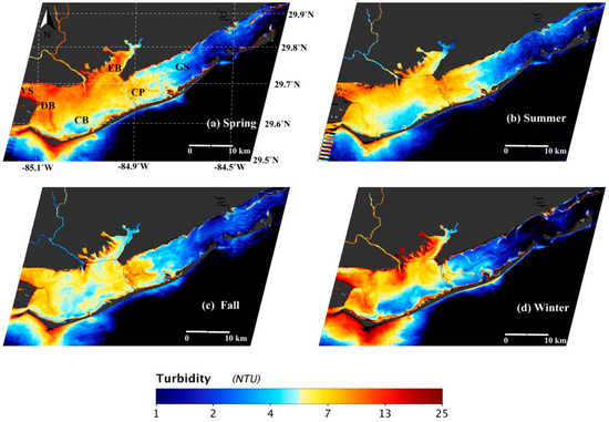
Figure 9.
Mean seasonal turbidity maps in Apalachicola Bay. (a) Spring (March, April, and May)—12 images; (b) summer (June, July, and August)—12 images; (c) fall (September and October)—13 images, and (d) winter (November, December, January, and February)—12 images. Data outside the seasonal reflectance and turbidity thresholds (as in Section 3.1.4) have been masked with black color. Clouds mask (ρband-7 > 0.011) is applied similar to Wang and Shi (2006) [76]. VS = St. Vincent Sound, DB = Dry Bar, CB = Central Bay, EB = East Bay, CP = Cat Point, and GS = St. George Sound.
3.3. Turbidity Maps during Extreme Events in Apalachicola Bay
The general turbidity algorithm was used with applications of season-dependent thresholds to convert atmospheric-corrected satellite images to the turbidity maps in Apalachicola Bay. Three extreme case scenarios were examined to investigate the effects of major physical forcings on the distribution of turbidity and water dynamics in the bay.
3.3.1. Apalachicola River Flood Conditions (4 April 2005 and 15 April 2009)
Landsat 5 TM images were obtained during two extreme case scenarios when (1) a peak river discharge (~4580 m3s−1) was observed in the strongest Apalachicola River flood event (April-2005) in the 8-year study period; and (2) the diminishing phase of river discharge (~1910 m3s−1) during the strong flood event in 2009 (also see Figure 6a). On 4 April 2005, Apalachicola River discharge was ~8 times higher than the mean discharge (~558 m3s−1) of study period (Figure 10a). Tidal height indicated flooding phase approaching to slack water, and northwesterly winds were relatively weaker (~2 ms−1) to play significant role in bay’s water dynamics (Figure 10c). Turbidity map showed highly turbid water mass (>50 NTU) in central bay directed towards the east, and gradually diluted by the saline Gulf water entering through the East Pass (Figure 10e). Apalachicola Bay experienced longer period of ebb tidal phase just few hours before the image acquisition. Although the tidal range was small, a combination of ebb tidal currents and high river discharge could have drawn significant amount of water in the central bay that later could have been trapped inside the bay due to shorter transition period from ebb to successive flood tidal phase. Flooding-supported intrusion of less turbid saline waters through the West and Indian passes is clearly evident in the maps. Furthermore, St. George Sound is relatively deeper than St. Vincent Sound [72]. Therefore, west to east surface gradient and increasing tidal height could have caused the net eastward movement of turbid fresh water plume during the image acquisition. Interestingly, distinct dark colored water enters from the marshes, Tate’s hell long-leaf pine forest (East Bay), and the Carrabelle River plume to the bay (See Figure 1). This CDOM-rich water has been masked out in the turbidity map.
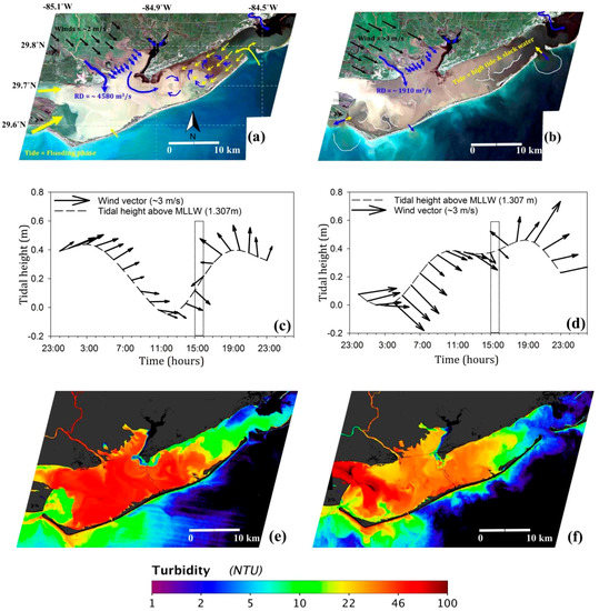
Figure 10.
(a–f) A true color image (top), tidal-height and wind time-series (center), and turbidity map (bottom) for the Apalachicola River flood condition on 4 April 2005 (left panel) and on 15 April 2009 (right panel).
Second case represents the influence of wind speed and river discharge during low energy (slack water) and high tidal period (Figure 10b). The bay experienced sustained periods of moderate northwesterly winds (>3 ms−1) during the flooding phase before image acquisition (Figure 10d). Hence, a distinct feature of turbid water mass in St. Vincent Sound could be an outcome of wind induced sediment re-suspension rather than the river supplied sediments possibly due to the relatively shallower depths of this region. Furthermore, tidal forcing was weak during the image acquisition, and hence moderate exchange of turbid river plume could have occurred via the West Pass and Sikes Cut despite high tides in the bay (Figure 10f). Moreover, high tidal phase could have caused a two-layered water column at the inlets with relatively low-density river water exiting the bay over underlying denser saline water. The eastward transport, mixing, and dilution of sediment rich water were similar as observed in the previous case.
3.3.2. Passages of Strong Cold Fronts over Apalachicola Bay (12 January 2010 and 13 February 2010)
In winter and early spring, Apalachicola Bay experiences frequent passages of southward propagating high-pressure systems characterized by cold air temperatures and strong winds. This scenario is represented by two cases, (1) a remnant of a strong frontal system that passed on 9 January 2010; and (2) a passage of strong frontal system on 13 February 2010. On 12 January 2010, a frontal remnant passed over the bay in the morning, and moderate northwesterly winds (>2.5 ms−1) sustained throughout the day. Furthermore, the bay experienced a severe “cold stun” event (7–14 January 2010) when water temperature fell below 10 °C affecting marine life for several days [77]. Apalachicola River discharge was about 1.5 times higher than the mean discharge of study period (Figure 11a). There were no records of precipitation over the bay within a time span of 3 days before image acquisition. Tidal height distribution showed flooding phase, however, to be relatively weaker during this time of a year as discussed in the temporal analysis (Figure 7d and Figure 11c). The elevated river discharge in absence of precipitation indicated influence of sustained winds that could have drawn off the river water and increased water turbidity in the bay due to mixing and re-suspension. Furthermore, northwesterly winds could have directed turbid plume water towards the barrier islands from where it could have been further diverted to the east towards St. George Sound and to the west towards central bay. Although water level in the bay was relatively high at the end of flood tidal phase, wind supported salt-water intrusion and shallower depths of the western region could have blocked the plume from escaping freely through the West Pass. This hypothetical view is further supported by turbidity patterns in the map that could have occurred due to strong interactions between turbid fresh water mass and a relatively clear marine water mass in central bay (Figure 11e). The net water movement could have occurred towards relatively deeper St. George Sound. The effect of flooding phase is clearly evident as intrusion of less turbid and saline water through the East Pass and Sikes Cut.
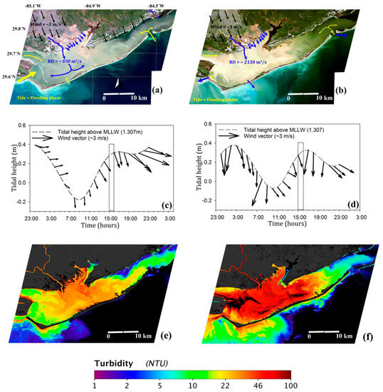
Figure 11.
(a–f) A true color image (top), tidal-height and wind time-series (center), and turbidity map (bottom) during the cold-front passages on 12 January 2010 (left panel) and on 13 February 2010 (right panel).
On 13 February 2010, a strong frontal system passed over Apalachicola Bay. The river discharge was 4 times higher than the mean discharge in the bay (Figure 11b). Apalachicola Bay experienced anomalously higher precipitation since the beginning of the year 2010 with ~16 mm of rain on the day of image acquisition. During winter and early spring, the anomalously high rainfall events in the southwest USA have been previously associated to the ENSO [74,75]. The year 2009–2010 experienced a moderate El Niño event that can be linked to the change in precipitation and river discharge pattern in the Apalachicola Basin. Also, the bay experienced moderate northerly winds that prevailed much longer before image acquisition (Figure 11d). Therefore, river plume dynamics could have been similar to the previous case. However, turbid water could have to escape through the West Pass, the East Pass, and Sikes Cut despite the flooding phase possibly due to unique combination of wind and river forcing. The highest turbidity was generally observed over the shallow regions of the bay, e.g., oyster bars, possibly due to sediment re-suspension, although the turbidity was masked because it exceeded the reflectance thresholds generally observed during winter (Figure 11f).
3.3.3. Low Flow Conditions in Apalachicola Bay
This scenario represents two cases, (1) the effect of a tropical storm during low flow condition on 8 September 2004; and (2) a strong frontal passage during low flow conditions on 22 November 2008. The first case shows turbidity map two days after the Hurricane Frances that made landfall to the East of Apalachicola Bay on 6 September 2004, when river discharge was ~50% lower than the average discharge (~558 m3s−1) of the study period (Figure 12a). As expected, the bay experienced sustained periods of southwesterly winds—as generally observed to the southwest of tropical storms. Tidal height showed the beginning of ebb tidal phase during the image acquisition (Figure 12c). However, winds could have been more dominant than the tidal forcing near the West and Indian passes, which could have veered the turbid river plume towards East Bay and St. George Sound (Figure 12e). Overall, the well-mixed nature of the bay indicated the dominance of storm-induced southerly winds during low flow conditions. Chen et al. (2009) used MODIS high-resolution imagery to generate total suspended solids (TSS) maps, and studied the effects of Hurricane Frances in Apalachicola Bay. They observed similar patterns of total suspended solids and southwesterly winds after the passage of Hurricane Frances.

Figure 12.
(a–f) A true color image (top), tidal-height and wind time-series (center), and turbidity map (bottom) after a hurricane passage on 8 September 2004 (left panel) and during frontal passage in low flow condition on 22 November 2008 (right panel).
In the second case, a strong frontal system passed perpendicular to the Apalachicola River. The strongest winds (>6 ms−1) were observed among all the cases, however river discharge was ~50% lower than the mean discharge of ~558 m3s−1 (Figure 12b). In contrast to the northwesterly winds, perpendicular forcing of the northeasterly winds could have confined the river water to the river channel. Interestingly, river discharge was higher before and after the cold front, whereas it decreased during the frontal passage. Despite the ebb tidal phase, wind could have supported the water intrusion through the East Pass, and net water movement from the East to West (Figure 12d). Turbidity was the highest in the shallower parts of central bay (e.g., Dry Bar) possibly due to wind-induced sediment re-suspension and sediment transport from St. George Sound and East Bay (Figure 12f).
4. Assessing Potential Applicability of Turbidity Algorithm to Landsat 8 OLI
Landsat 8 OLI, a successor of Landsat 5 TM and Landsat 7 ETM+ sensors, contains spectral bands similar to its predecessors except additional channels in deep blue (430–450 nm) and infrared (1360–1380 nm) spectral regions that further improve its capability in monitoring water resources and cirrus cloud detection. In addition, the signal-to-noise ratio and radiometric resolution (12 bits) of OLI were higher than Landsat 5 TM (8 bits). The OLI red band has a better spectral resolution (640–670 nm, bandwidth = 30 nm) than Landsat 5 TM (630–690 nm, bandwidth = 60 nm). Furthermore, the red band is located just outside chlorophyll-a absorption peak which might reduce the chlorophyll contamination to the particulate back-scattered signal and hence, Landsat 5 TM—turbidity relationship could be applicable to Landsat 8 OLI. A set of FLAASH-corrected 17 clear-sky Landsat 8 OLI images (Table S3) were converted to turbidity using the proposed single band empirical relationship. The matchup comparison between modeled and in situ turbidity showed promising results along with turbidity maps as illustrated in Figure 13. Turbidity maps represent images for 3 seasons: winter (18 February 2015) (Figure 13b), spring (8 March 2016) (Figure 13c), and summer (7 July 2016) (Figure 13d). In spring, river discharge was approximately two and three folds higher (~1050 m3/s) than in winter and summer, respectively. However, wind speed and direction appears to be major controlling factors of the bay’s water dynamics and turbidity distribution despite elevated river discharge in the spring and the winter. Interestingly, these individual images are also matching with seasonally averaged turbidity maps (Figure 6), further supporting the applicability of the Landsat 5 TM-based turbidity algorithm to Landsat 8 OLI, and its potential for long-term monitoring of water turbidity in a shallow water estuary such as Apalachicola Bay.
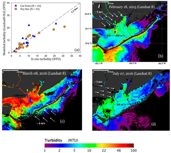
Figure 13.
(a) Performance of Landsat 5 TM-based red band empirical relationship on Landsat 8 OLI images (R2 = 0.80, N = 31); (b–d) Turbidity maps derived using Landsat 8 OLI imagery (18 February 2015, 08 March 2016, and 7 July 2016, respectively) and the general turbidity algorithm. Reflectance values beyond seasonal thresholds and clouds are masked in the maps.
5. Conclusions
Apalachicola Bay is a bar-built estuary located to the west of Florida’s panhandle and is well-known for its commercial oyster yields. We investigated turbidity climatology (2004–2011) to understand roles of meteorological, hydrological and astronomical factors on the bay’s water dynamics and turbidity distribution. Together, time-series, PCA, and classification tree-based analysis conveyed important information that the bay is highly dynamic in nature, both diurnally and seasonally, and its water quality (e.g., turbidity) is largely driven by interactions of different physical forcings, such as river discharge, tides, winds, and precipitation associated run-off, except during the extreme conditions when one or more of these factors become the dominant regulator of the bay’s water dynamics (e.g., river flood, cold fronts, and tropical storms). The following conclusions can be derived from the temporal analysis of physical forcings in Apalachicola Bay:
(1) Apalachicola Bay, especially the western and eastern sides of river mouth, experiences higher turbidity in the spring and the winter mainly due to elevated supply of sediments by the Apalachicola River and wind-induced sediment re-suspension and mixing of the shallow water column. In addition, periods of strong winds, mainly associated with the passage of low-pressure systems (e.g., storms and hurricanes), can result in higher flow velocity and increased water turbidity for a few days under low flow conditions in summer and fall [14,41].
(2) Apalachicola River discharge and wind speed were the major influential forcing at Cat Point (the eastern region) station, but tidal height could be the common factor for the variations in diurnal turbidity especially in the St. George Sound possibly due to the strong influence of semi-diurnal tides and its remoteness to the fresh water sources [38,39]. In contrast, all the forcings were relatively important at Dry Bar (the western region) due to its shallower depths and proximity to major inlets and land.
(3) The study of water dynamics and turbidity distribution is highly complex due to the multiple inlets and strong interactions of major physical forcings in Apalachicola Bay. The water dynamics is mainly controlled by the interactions of three forces: river discharge, tide, and winds. River plume generally flow from north to south with tendency to escape the bay through the closest inlet, the West Pass. In contrast, tides and winds either control the free flow of river plume either by blocking/diverting it in the opposite direction or by assisting the river mass to escape through the tidal inlets.
Landsat sensors (e.g., TM, ETM+, and OLI) are mainly designed for land application; however they can be utilized to investigate estuarine water dynamics and turbidity distribution. We have used ENVI’s FLAASH-based atmospheric correction, as it is a crucial step in ocean color remote sensing. However, the validation of FLAASH performance was necessary before using the atmospheric-corrected Landsat reflectance in the algorithm development. FLAASH-AERONET comparison yielded promising results to provide enough confidence for using FLAASH-derived surface reflectance in low to moderately turbid waters in Apalachicola Bay. Although this comparison contains many errors mainly due to the effects of skylight, it gave a preliminary indication of reasonable performance of the FLAASH. We have explored historical archives of Landsat 5 TM and in situ turbidity measurements to develop a simple single band (Band 3: 630–690 nm) Landsat 5 TM—turbidity relationship in Apalachicola Bay. Bootstrap-based uncertainty analysis overall yielded a reasonable performance of a turbidity algorithm with realistic possibility of training and testing data sets (N = 5000 simulations). The bootstrap results provided reasonable estimates of a constant and power law exponent for a turbidity algorithm for the Apalachicola Bay. We also tested seasonal dependency of the Landsat 5 TM—turbidity relationship and found that the individual seasonal relationship deviates significantly from the general turbidity algorithm. Hence, we restricted the use of the turbidity algorithm to different seasons by applying seasonal thresholds. Seasonally-mean turbidity maps showed distinct patterns of turbidity in Apalachicola Bay with moderate to highly turbid waters in spring and winter, in contrast to low to moderately turbid waters in summer and fall. Shallow regions of the bay (e.g., East Bay, St. Vincent Sound, Cat Point Bar, and Dry Bar) remain turbid throughout the year while relatively deeper parts (e.g., Central Bay and St. George sound) of the bay remain clearer—except during strong winds and high fresh water inputs.
We presented synoptic views of three extreme case scenarios to examine water dynamics and turbidity distribution in Apalachicola Bay. Turbidity maps generally showed good agreement with the meteorological, hydrological, and astronomical forcings in the bay. The following results can be derived from these extreme case scenarios:
(1) Apalachicola River discharge is the major controlling factor on turbidity during the high-flow conditions. Winds may affect turbidity, especially in shallow regions of the bay, through sediment re-suspension and mixing, but only if it prevails over longer periods. Tidal-influence mainly depends on the flood and ebb tidal phases, except during the slack waters when tidal forcing is weak. The flood tides increase the tidal height by introducing saline water in the bay, whereas ebb tides decrease the tidal height by drawing water out of the bay. Turbidity maps indicated that the synchronization of ebb tidal flow and river discharge during high river flow conditions may have stronger effects on bay’s water turbidity than the combination of river discharge and flood tides – which can cause dilution of the bay’s water.
(2) Apalachicola Bay experiences strong northerly winds during the passage of cold-frontal systems. The sustained winds can increase water turbidity by drawing off the river water and by re-suspending sediments in shallow regions of the bay. Similarly, anomalously high precipitation and associated run-off can further increase water turbidity in the bay. Westerly and easterly components of northerly winds can divert river plume waters to different regions of the bay. Likewise, flood and ebb tidal phases affect the sediment transport and its exchange to the shelf. Overall, Apalachicola Bay experiences extremely turbid environments when two forcings, winds and river flow, are in phase.
(3) Wind becomes the dominant factor controlling water dynamics during low flow conditions. The bay becomes well-mixed and relatively saline after the passage of tropical storms and hurricanes. However, the bay’s turbidity depends on the strength of winds. Furthermore, if strong winds move perpendicular to the river channel, it can reduce the freshwater input to the bay by confining river water within the river channel.
Turbidity maps showed reasonable performance of a turbidity algorithm in Apalachicola Bay; however several issues may have affected the performance of the algorithm that still needs to be addressed. These include the following: (1) contamination of signal by the bottom reflectance; (2) interference due to high concentrations of CDOM; (3) instrumentation error in in situ measurements; (4) sensor calibration; (5) contributions from skylight and sun-glint on the surface reflectance products; (6) performance of the atmospheric correction module and; (7) simplistic assumptions of water column homogeneity. The aim of this study was to investigate the turbidity climatology in Apalachicola Bay and thus, historic Landsat 5 TM data were used in the analysis. The performance of single-band empirical relationships showed promising results on more advanced instruments (e.g., Landsat 8 OLI) and its applicability should be further explored in other coastal regions using much robust ocean color parameters (e.g., remote sensing reflectance (Rrs)). Although the proposed algorithm has been shown to work well in Apalachicola Bay, it could be subject to change in band combination, coefficients, and/or regression function, if it is used in other coastal regions. Nonetheless, the promising performance of the empirical Landsat 5 TM—turbidity relationship supports the use of Landsat data in monitoring water quality in estuarine environments.
Supplementary Materials
The following are available online at www.mdpi.com/2072-4292/9/4/367/s1, Figure S1: Landsat 5 TM turbidity algorithm with NIR band (Band 4), Figure S2: Turbidity-Landsat 5 TM relationships for different seasons. Blue and orange symbols represent measurements at Cat Point and Dry Bar stations, Figure S3: Bootstrap simulation (N = 5000) results, (a) intercept or log (constant) (Mean ± SD = 8.32 ± 0.50, range = 6.2–10.16), (b) slope or power law exponent (Mean ± SD = 1.76 ± 0.14, range = 1.16–2.35), c) R2 for turbidity-Landsat 5 TM algorithm, (d) R2 for algorithm validation, (e) RMSE for algorithm validation, and (f) bias for algorithm validation., Figure S4: Histogram of mean-daily Apalachicola River discharge from 2004 to 2011, Figure S5: Decomposition of precipitation time-series (2004–2011) into, (a) daily (N = 2439 days), (b) seasonal, (c) yearly trend, (d) random or remainder component (=daily time-series − (seasonal component + yearly trend)), Figure S6: Time-series of turbidity was decomposed into seasonal, trend, and random components for recognizing the underlying pattern during the 8-years of study period at Cat Point station, Figure S7: The turbidity time-series at Dry Bar was decomposed after removing outliers, Table S1: Bootstrapping statistics for the turbidity algorithm and its validation, Table S2: Sample size, mean, standard deviation, and range of mean-daily river discharge, precipitation, salinity, tidal height, wind speed, water depth, and turbidity from 2004 to 2011 in Apalachicola Bay, Table S3: Turbidity matchups at Cat Point and Dry Bar stations used to evaluate applicability of the Landsat 5 TM-based turbidity algorithm to Landsat 8 OLI images (17 images).
Acknowledgments
Authors acknowledge NASA funding (Project No. NNX14A043G). We would like to thank NOAA NERRS Centralized Data Management Office for the turbidity and meteorological data. We are also thankful to Alan Weidermann, Bill Gibson and Robert Arnone for the AERONET-Ocean color data and USGS for Landsat imagery.
Author Contributions
I.J. and E.D. conceived and designed the research; I.J. analyzed the data and drafted the work and all authors critically revised the paper for intellectual content.
Conflicts of Interest
The authors declare no conflict of interest.
References
- Cloern, J.E.; Foster, S.; Kleckner, A. Phytoplankton primary production in the world’s estuarine-coastal ecosystems. Biogeosciences 2014, 11, 2477–2501. [Google Scholar]
- Chelsea Nagy, R.; Graeme Lockaby, B.; Kalin, L.; Anderson, C. Effects of urbanization on stream hydrology and water quality: The Florida Gulf Coast. Hydrol. Process. 2012, 26, 2019–2030. [Google Scholar]
- Giosan, L.; Syvitski, J.; Constantinescu, S.; Day, J. Climate change: Protect the world’s deltas. Nature 2014, 516, 31–33. [Google Scholar] [CrossRef] [PubMed]
- Fabricius, K.E. Effects of terrestrial runoff on the ecology of corals and coral reefs: Review and synthesis. Mar. Pollut. Bull. 2005, 50, 125–146. [Google Scholar] [PubMed]
- Kenworthy, W.J.; Fonseca, M.S. Light requirements of seagrasses Halodule wrightii and Syringodium filiforme derived from the relationship between diffuse light attenuation and maximum depth distribution. Estuaries 1996, 19, 740–750. [Google Scholar]
- Pedersen, T.M.; Gallegos, C.L.; Nielsen, S.L. Influence of near-bottom re-suspended sediment on benthic light availability. Estuar. Coast. Shelf Sci. 2012, 106, 93–101. [Google Scholar] [CrossRef]
- Thrush, S.F.; Hewitt, J.E.; Cummings, V.J.; Ellis, J.I.; Hatton, C.; Lohrer, A.; Norkko, A. Muddy Waters: Elevating Sediment Input to Coastal and Estuarine Habitats. Front. Ecol. Environ. 2004, 2, 299–306. [Google Scholar]
- Ryan, P.A. Environmental effects of sediment on New Zealand streams: A review. N. Z. J. Mar. Freshw. Res. 1991, 25, 207–221. [Google Scholar]
- Wang, H.; Huang, W.; Harwell, M.A.; Edmiston, L.; Johnson, E.; Hsieh, P.; Milla, K.; Christensen, J.; Stewart, J.; Liu, X. Modeling oyster growth rate by coupling oyster population and hydrodynamic models for Apalachicola Bay, Florida, USA. Ecol. Model. 2008, 211, 77–89. [Google Scholar]
- Robertson, M.J.; Scruton, D.A.; Clarke, K.D. Seasonal effects of suspended sediment on the behavior of juvenile Atlantic salmon. Trans. Am. Fish. Soc. 2007, 136, 822–828. [Google Scholar]
- Pollock, F.J.; Lamb, J.B.; Field, S.N.; Heron, S.F.; Schaffelke, B.; Shedrawi, G.; Bourne, D.G.; Willis, B.L. Sediment and turbidity associated with offshore dredging increase coral disease prevalence on nearby reefs. PLoS ONE 2014, 9, e102498. [Google Scholar] [CrossRef] [PubMed]
- Rügner, H.; Schwientek, M.; Beckingham, B.; Kuch, B.; Grathwohl, P. Turbidity as a proxy for total suspended solids (TSS) and particle facilitated pollutant transport in catchments. Environ. Earth Sci. 2013, 69, 373–380. [Google Scholar] [CrossRef]
- Stubblefield, A.P.; Reuter, J.E.; Goldman, C.R. Sediment budget for subalpine watersheds, Lake Tahoe, California, USA. Catena 2009, 76, 163–172. [Google Scholar] [CrossRef]
- Chen, S.; Huang, W.; Wang, H.; Li, D. Remote sensing assessment of sediment re-suspension during Hurricane Frances in Apalachicola Bay, USA. Remote Sens. Environ. 2009, 113, 2670–2681. [Google Scholar] [CrossRef]
- D’Sa, E.J.; Ko, D.S. Short-term Influences on Suspended Particulate Matter Distribution in the Northern Gulf of Mexico: Satellite and Model Observations. Sensors 2008, 8, 4249–4264. [Google Scholar] [CrossRef] [PubMed]
- Kemker, C. Turbidity, Total Suspended Solids and Water Clarity. In Fundamentals of Environmental Measurements; Fondriest Environmental, Inc.: Fairborn, OH, USA, 2014; Available online: http://www.fondriest.com/environmental-measurements/parameters/water-quality/turbidity-total-suspended-solids-water-clarity/ (accessed on 30 August 2016).
- Mobley, C.; Boss, E.; Roesler, C. Ocean Optics Web Book. 2010. Available online: http://www.oceanopticsbook.info (accessed on15 March 2016).
- Dogliotti, A.; Ruddick, K.; Nechad, B.; Doxaran, D.; Knaeps, E. A single algorithm to retrieve turbidity from remotely-sensed data in all coastal and estuarine waters. Remote Sens. Environ. 2015, 156, 157–168. [Google Scholar] [CrossRef]
- Chen, Z.; Hu, C.; Muller-Karger, F. Monitoring turbidity in Tampa Bay using MODIS/Aqua 250-m imagery. Remote Sens. Environ. 2007, 109, 207–220. [Google Scholar] [CrossRef]
- Choi, J.K.; Park, Y.J.; Ahn, J.H.; Lim, H.S.; Eom, J.; Ryu, J.H. GOCI, the world’s first geostationary ocean color observation satellite, for the monitoring of temporal variability in coastal water turbidity. J. Geophys. Res. Oceans 2012, 117. [Google Scholar] [CrossRef]
- Miller, R.L.; McKee, B.A. Using MODIS Terra 250 m imagery to map concentrations of total suspended matter in coastal waters. Remote Sens. Environ. 2004, 93, 259–266. [Google Scholar] [CrossRef]
- Minella, J.P.; Merten, G.H.; Reichert, J.M.; Clarke, R.T. Estimating suspended sediment concentrations from turbidity measurements and the calibration problem. Hydrol. Process. 2008, 22, 1819–1830. [Google Scholar] [CrossRef]
- Onderka, M.; Pekárová, P. Retrieval of suspended particulate matter concentrations in the Danube River from Landsat ETM data. Sci. Total Environ. 2008, 397, 238–243. [Google Scholar] [CrossRef] [PubMed]
- Zhang, M.; Tang, J.; Dong, Q.; Song, Q.; Ding, J. Retrieval of total suspended matter concentration in the Yellow and East China Seas from MODIS imagery. Remote Sens. Environ. 2010, 114, 392–403. [Google Scholar] [CrossRef]
- Gippel, C.J. Potential of turbidity monitoring for measuring the transport of suspended solids in streams. Hydrol. Process. 1995, 9, 83–97. [Google Scholar] [CrossRef]
- D’Sa, E.J.; Miller, R.L.; McKee, B.A. Suspended particulate matter dynamics in coastal waters from ocean color: Application to the Northern Gulf of Mexico. Geophys. Res. Lett. 2007, 34, L23611. [Google Scholar] [CrossRef]
- Palmer, S.C.J.; Kutser, T.; Hunter, P.D. Remote sensing of inland waters: Challenges, progress and future directions. Remote Sens. Environ. 2015, 157, 1–8. [Google Scholar] [CrossRef]
- D’Sa, E.J.; Roberts, H.H.; Allahdadi, M.N. Suspended particulate matter dynamics along the Louisiana-Texas coast from satellite observation. In Proceedings of the Coastal Sediments 2011, Miami, FL, USA, 2–6 May 2011; Rosati, J.D., Wang, P., Roberts, T.M., Eds.; pp. 2390–2402. [Google Scholar]
- Edmiston, H. A River Meets the Bay—A Characterization of the Apalachicola River and Bay System. Apalachicola National Estuarine Research Reserve; Florida Department of Environmental Protection: Tallahassee, FL, USA, 2008; pp. 1–200. [Google Scholar]
- Leitman, H.M.; Sohm, J.E.; Franklin, M.A. Wetland Hydrology and Tree Distribution of the Apalachicola River Flood Plain, Florida; US Geological Survey: Reston, VA, USA, 1984.
- Whitfield, W.; Beaumariage, D.S. Shellfish management in Apalachicola Bay: Past, Present, Future. In Proceedings of the Conference on the Apalachicola Drainage System, Gainesville, FL, USA, 23–24 April 1977; Florida Department of Natural Resources Marine Research Laboratory: Gainesville, FL, USA, 1977; pp. 130–140. [Google Scholar]
- Havens, K.; Allen, M.; Camp, E.; Irani, T.; Lindsey, A.; Morris, J.; Kane, A.; Kimbro, D.; Otwell, S.; Pine, B. Apalachicola Bay Oyster Situation Report; Florida Sea Grant College Program, Technical Publication TP-200; Florida Sea Grant: Gainesville, FL, USA, 2013; Available online: https://www.flseagrant.org/news/2013/04/apalachicola-oyster-report/ (accessed on 20 May 2016).
- Edmiston, H.L.; Fahrny, S.A.; Lamb, M.S.; Levi, L.K.; Wanat, J.M.; Avant, J.S.; Wren, K.; Selly, N.C. Tropical Storm and Hurricane Impacts on a Gulf Coast Estuary: Apalachicola Bay, Florida. J. Coast. Res. 2008, 38–49. [Google Scholar] [CrossRef]
- Grattan, L.M.; Roberts, S.; Mahan, W.T., Jr.; McLaughlin, P.K.; Otwell, W.S.; Morris, J.G., Jr. The Early Psychological Impacts of the Deepwater Horizon Oil Spill on Florida and Alabama Communities. Environ. Health Perspect. 2011, 119, 838–843. [Google Scholar] [CrossRef] [PubMed]
- Petes, L.E.; Brown, A.J.; Knight, C.R. Impacts of upstream drought and water withdrawals on the health and survival of downstream estuarine oyster populations. Ecol. Evol. 2012, 2, 1712–1724. [Google Scholar] [CrossRef] [PubMed]
- Livingston, R.J. Climate Change and Coastal Ecosystems: Long-Term Effects of Climate and Nutrient Loading on Trophic Organization; CRC Press: Boca Raton, FL, USA, 2014. [Google Scholar]
- Surratt, D.; Cherrier, J.; Robinson, L.; Cable, J. Chronology of sediment nutrient geochemistry in Apalachicola Bay, Florida (U.S.A). J. Coast. Res. 2008, 24, 660–671. [Google Scholar] [CrossRef]
- Koch, M.; Sun, H. Tidal and Non-Tidal Characteristics of water Levels and Flow in the Apalachicola Bay, Florida. WIT Trans. Built Environ. 1970, 43, 357–366. [Google Scholar] [CrossRef]
- Huang, W.; Sun, H.; Nnaji, S.; Jones, W. Tidal Hydrodynamics in a Multiple-Inlet Estuary: Apalachicola Bay, Florida. J. Coast. Res. 2002, 674–684. [Google Scholar]
- Huang, W.; Chen, S.; Yang, X. Remote sensing for water quality monitoring in Apalachicola Bay, USA. In Advances in Earth Observation of Global Change; Chuvieco, E., Li, J., Yang, X., Eds.; Springer: Dordrecht, The Netherlands, 2010; pp. 69–78. [Google Scholar]
- Liu, X.; Huang, W. Modeling sediment resuspension and transport induced by storm wind in Apalachicola Bay, USA. Environ. Model. Softw. 2009, 24, 1302–1313. [Google Scholar] [CrossRef]
- Hu, C.; Chen, Z.; Clayton, T.D.; Swarzenski, P.; Brock, J.C.; Muller–Karger, F.E. Assessment of estuarine water-quality indicators using MODIS medium-resolution bands: Initial results from Tampa Bay, FL. Remote Sens. Environ. 2004, 93, 423–441. [Google Scholar] [CrossRef]
- Gordon, H.R.; Wang, M. Retrieval of water-leaving radiance and aerosol optical thickness over the oceans with SeaWiFS: A preliminary algorithm. Appl. Opt. 1994, 33, 443–452. [Google Scholar] [CrossRef] [PubMed]
- Chavez, P.S. Image- based atmospheric corrections-revisited and improved. Photogramm. Eng. Remote Sens. 1996, 62, 1025–1035. [Google Scholar]
- Hu, C.; Carder, K.L.; Muller-Karger, F.E. Atmospheric correction of SeaWiFS imagery over turbid coastal waters: A practical method. Remote Sens. Environ. 2000, 74, 195–206. [Google Scholar] [CrossRef]
- Ruddick, K.G.; Ovidio, F.; Rijkeboer, M. Atmospheric correction of SeaWiFs imagery for turbid coastal and inland waters. Appl. Opt. 2000, 39, 897–912. [Google Scholar] [CrossRef] [PubMed]
- Siegel, D.A.; Wang, M.; Maritorena, S.; Robinson, W. Atmospheric Correction of Satellite Ocean Color Imagery: The Black Pixel Assumption. Appl. Opt. 2000, 39, 3582–3591. [Google Scholar] [CrossRef] [PubMed]
- Wang, M.; Shi, W. The NIR-SWIR combined atmospheric correction approach for modis ocean color data processing. Opt. Express 2007, 15, 15722–15733. [Google Scholar] [CrossRef] [PubMed]
- Adler-Golden, S.; Berk, A.; Bernstein, L.; Richtsmeier, S.; Acharya, P.; Matthew, M.; Anderson, G.; Allred, C.; Jeong, L.; Chetwynd, J. FLAASH, a MODTRAN4 atmospheric correction package for hyperspectral data retrievals and simulations. In Proceedings of the 7th Ann. JPL Airborne Earth Science Workshop, Pasadena, CA, USA, 12–16 January 1998; pp. 9–14. [Google Scholar]
- Kaufman, Y.; Wald, A.; Remer, L.; Gao, B.-C.; R-R, L.; Flynn, L. The MODIS 2.1-μm channel-correlation with visible reflectance for use in remote sensing of aerosol. IEEE Trans. Geosci. Remote Sens. 1997, 35, 1286–1298. [Google Scholar] [CrossRef]
- Joshi, I.; D’Sa, E.J. Seasonal Variation of Colored Dissolved Organic Matter in Barataria Bay, Louisiana, Using Combined Landsat and Field Data. Remote Sens. 2015, 7, 12478–12502. [Google Scholar] [CrossRef]
- Wilson, R.; Milton, E.; Nield, J. Are visibility-derived aot estimates suitable for parameterizing satellite data atmospheric correction algorithms? Int. J. Remote Sens. 2015, 36, 1675–1688. [Google Scholar] [CrossRef]
- Thuillier, G.; Hersé, M.; Foujols, T.; Peetermans, W.; Gillotay, D.; Simon, P.; Mandel, H. The solar spectral irradiance from 200 to 2400 nm as measured by the SOLSPEC spectrometer from the ATLAS and EURECA missions. Sol. Phys. 2003, 214, 1–22. [Google Scholar] [CrossRef]
- Gordon, H.R. Atmospheric correction of ocean color imagery in the Earth Observing System era. J. Geophys. Res. Atmos. 1997, 102, 17081–17106. [Google Scholar]
- Cleveland, R.B.; Cleveland, W.S.; McRae, J.E.; Terpenning, I. Stl: A Seasonal-Trend Decomposition Procedure Based on Loess. J. Off. Stat. 1990, 6, 3–73. [Google Scholar]
- Breiman, L.; Friedman, J.; Stone, C.J.; Olshen, R.A. Classification and Regression Trees; CRC Press: Boca Raton, FL, USA, 1984. [Google Scholar]
- De’ath, G.; Fabricius, K.E. Classification and Regression Trees: A Powerful Yet Simple Technique for Ecological Data Analysis. Ecology 2000, 81, 3178–3192. [Google Scholar] [CrossRef]
- Zhang, Y.; Liu, X.; Qin, B.; Shi, K.; Deng, J.; Zhou, Y. Aquatic vegetation in response to increased eutrophication and degraded light climate in Eastern Lake Taihu: Implications for lake ecological restoration. Sci. Rep. 2016, 6. [Google Scholar] [CrossRef] [PubMed]
- Efron, B.; Tibshirani, R.J. An Introduction to the Bootstrap; CRC Press: Boca Raton, FL, USA, 1994. [Google Scholar]
- Montgomery, D.C.; Peck, E.A.; Vining, G.G. Introduction to Linear Regression Analysis; John Wiley & Sons: Somerset, NJ, USA, 2015. [Google Scholar]
- Mortazavi, B.; Iverson, R.L.; Landing, W.M.; Lewis, F.G.; Huang, W. Control of phytoplankton production and biomass in a river-dominated estuary: Apalachicola Bay, Florida, USA. Mar. Ecol. Prog. Ser. 2000, 198, 19–31. [Google Scholar] [CrossRef]
- Del Castillo, C.E.; Gilbes, F.; Coble, P.G.; Müller-Karger, F.E. On the dispersal of riverine colored dissolved organic matter over the West Florida Shelf. Limnol. Oceanogr. 2000, 45, 1425–1432. [Google Scholar] [CrossRef]
- Gordon, H.R.; Lewis, M.R.; McLean, S.D.; Twardowski, M.S.; Freeman, S.A.; Voss, K.J.; Boynton, G.C. Spectra of particulate backscattering in natural waters. Opt. Express 2009, 17, 16192–16208. [Google Scholar] [CrossRef] [PubMed]
- Slade, W.H.; Boss, E. Spectral attenuation and backscattering as indicators of average particle size. Appl. Opt. 2015, 54, 7264–7277. [Google Scholar] [CrossRef] [PubMed]
- Fan, C.; Warner, R.A. Characterization of water reflectance spectra variability: Implications for hyperspectral remote sensing in estuarine waters. Mar. Sci. 2014, 4, 1–9. [Google Scholar]
- Joshi, I.D.; D’Sa, E.J.; Osburn, C.L.; Bianchi, T.S.; Ko, D.S.; Oviedo-Vargas, D.; Arellano, A.R.; Ward, N.D. Assessing chromophoric dissolved organic matter (CDOM) distribution, stocks, and fluxes in Apalachicola Bay using combined field, VIIRS ocean color, and model observations. Remote Sens. Environ. 2017, 191, 359–372. [Google Scholar] [CrossRef]
- Doxaran, D.; Froidefond, J.-M.; Castaing, P.; Babin, M. Dynamics of the turbidity maximum zone in a macrotidal estuary (the Gironde, France): Observations from field and MODIS satellite data. Estuar. Coast. Shelf Sci. 2009, 81, 321–332. [Google Scholar] [CrossRef]
- Wang, H.; Hladik, C.M.; Huang, W.; Milla, K.; Edmiston, L.; Harwell, M.; Schalles, J.F. Detecting the spatial and temporal variability of chlorophyll-a concentration and total suspended solids in Apalachicola Bay, Florida using MODIS imagery. Int. J. Remote Sens. 2010, 31, 439–453. [Google Scholar] [CrossRef]
- Bustamante, J.; Pacios, F.; Díaz-Delgado, R.; Aragonés, D. Predictive models of turbidity and water depth in the Doñana marshes using Landsat TM and ETM+ images. J. Environ. Manag. 2009, 90, 2219–2225. [Google Scholar] [CrossRef] [PubMed]
- Pope, R.M.; Fry, E.S. Absorption spectrum (380–700 nm) of pure water. II. Integrating cavity measurements. Appl. Opt. 1997, 36, 8710–8723. [Google Scholar] [CrossRef] [PubMed]
- Novoa, S.; Doxaran, D.; Ody, A.; Vanhellemont, Q.; Lafon, V.; Lubac, B.; Gernez, P. Atmospheric corrections and multi-conditional algorithm for multi-sensor remote sensing of suspended particulate matter in low-to-high turbidity levels coastal waters. Remote Sens. 2017, 9, 61. [Google Scholar] [CrossRef]
- Twichell, D.; Edmiston, L.; Andrews, B.; Stevenson, W.; Donoghue, J.; Poore, R.; Osterman, L. Geologic controls on the recent evolution of oyster reefs in Apalachicola Bay and St. George Sound, Florida. Estuar. Coast. Shelf Sci. 2010, 88, 385–394. [Google Scholar] [CrossRef]
- Reichstetter, M.; Fearns, P.R.; Weeks, S.J.; McKinna, L.I.; Roelfsema, C.; Furnas, M. Bottom Reflectance in Ocean Color Satellite Remote Sensing for Coral Reef Environments. Remote Sens. 2015, 7, 16756–16777. [Google Scholar] [CrossRef]
- Schmidt, N.; Lipp, E.; Rose, J.; Luther, M. ENSO influences on Seasonal Rainfall and River Discharge in Florida. J. Clim. 2001, 14, 615–628. [Google Scholar] [CrossRef]
- Sittel, M.C. Marginal Probabilities of the Extremes of ENSO Events for Temperature and Precipitation in the Southeastern United States; Center for Ocean-Atmosphere Prediction Studies, Florida State University: Tallahassee, FL, USA, 1994. [Google Scholar]
- Wang, M.; Shi, W. Cloud Masking for Ocean Color Data Processing in the Coastal Regions. IEEE Trans. Gesci. Remote Sens. 2006, 44, 3196–3205. [Google Scholar] [CrossRef]
- Roberts, K.; Collins, J.; Paxton, C.H.; Hardy, R.; Downs, J. Weather patterns associated with green turtle hypothermic stunning events in St. Joseph Bay and Mosquito Lagoon, Florida. Phys. Geogr. 2014, 35, 134–150. [Google Scholar] [CrossRef]
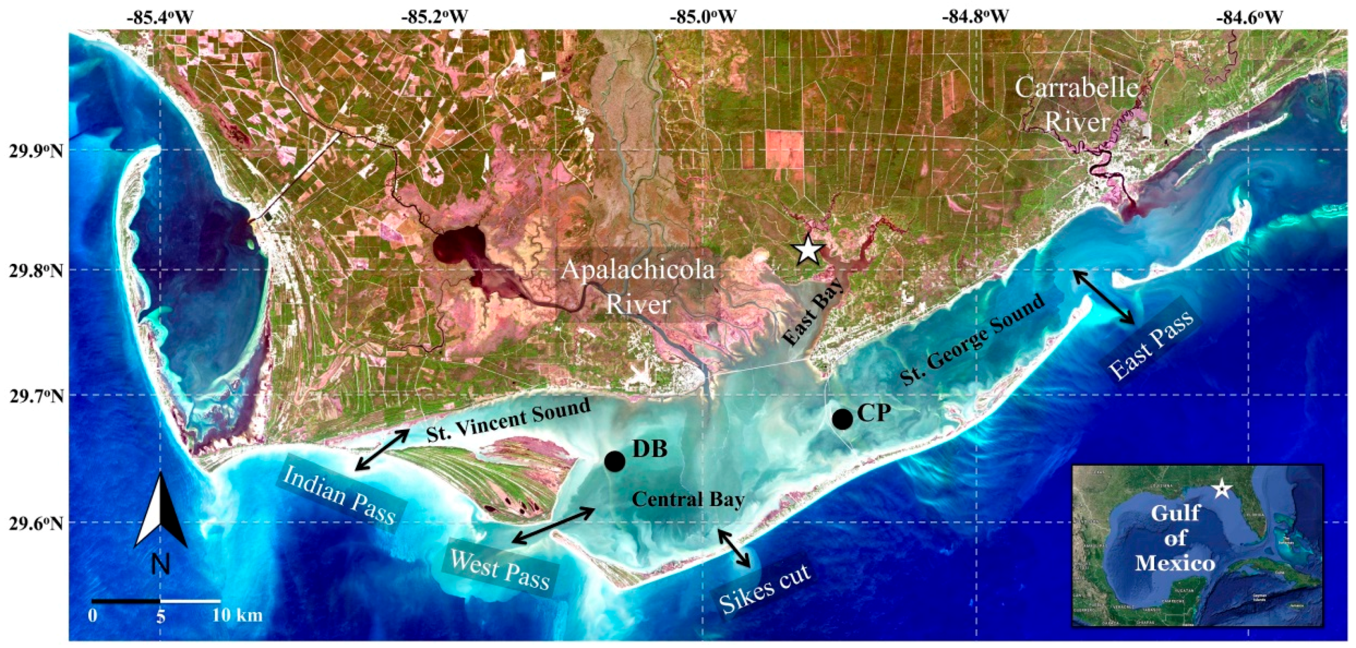

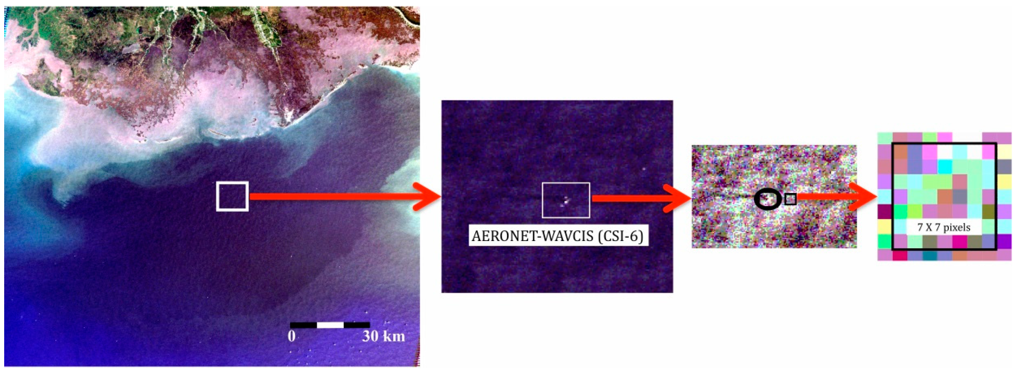
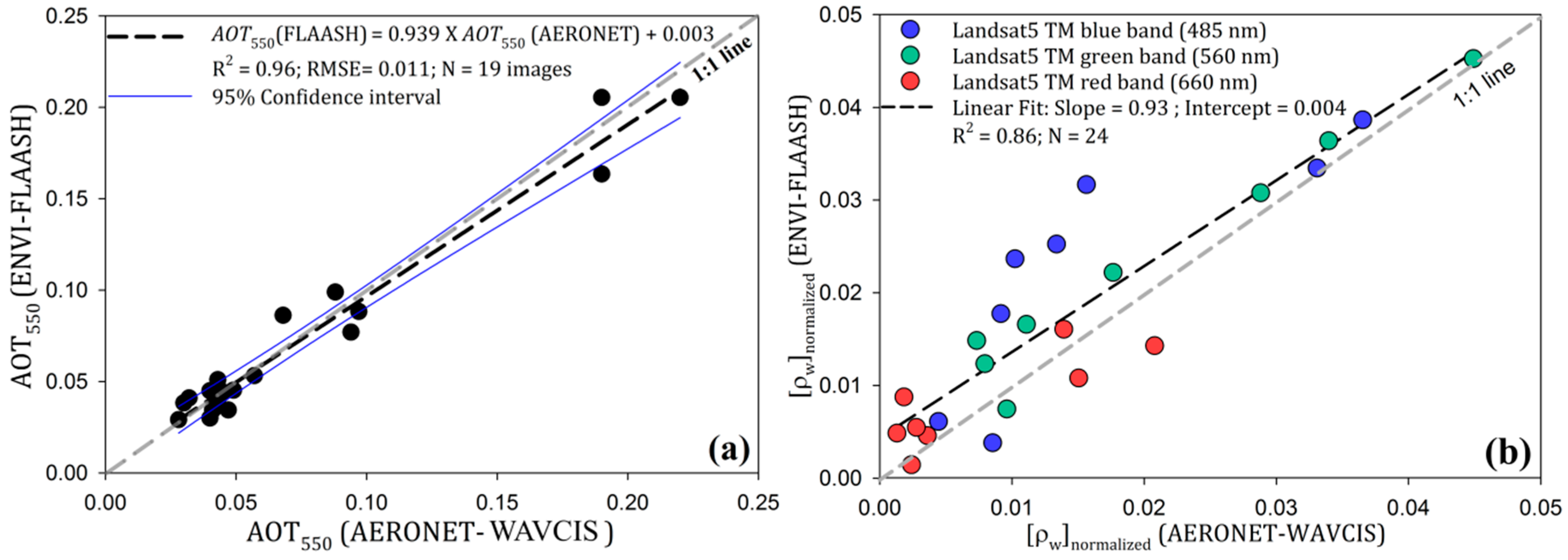
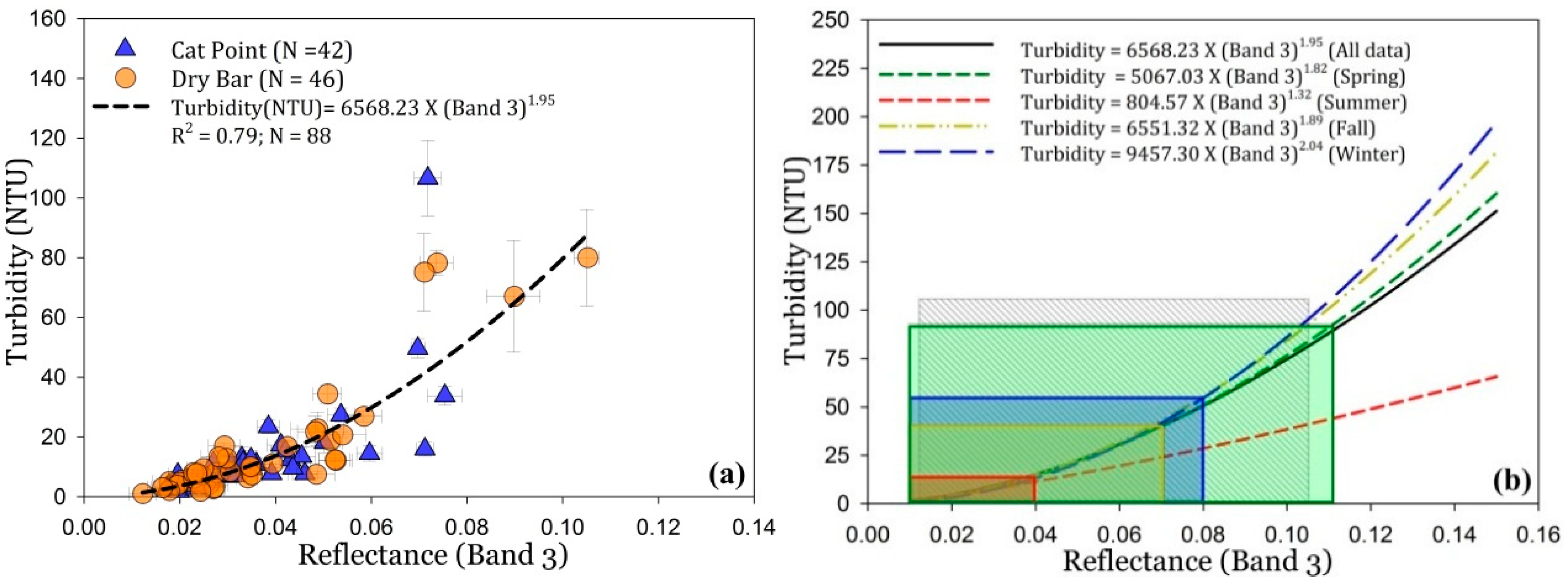
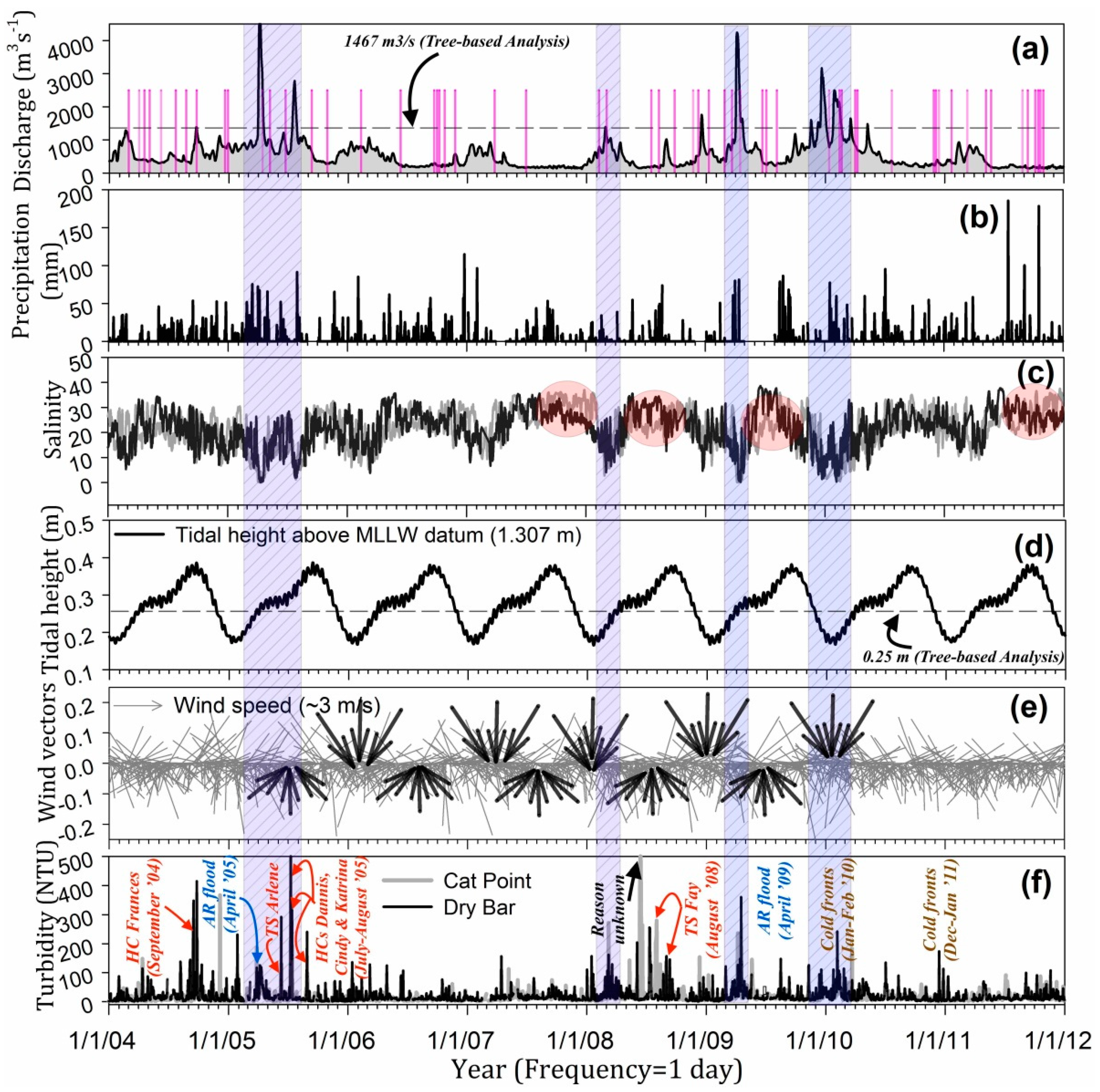
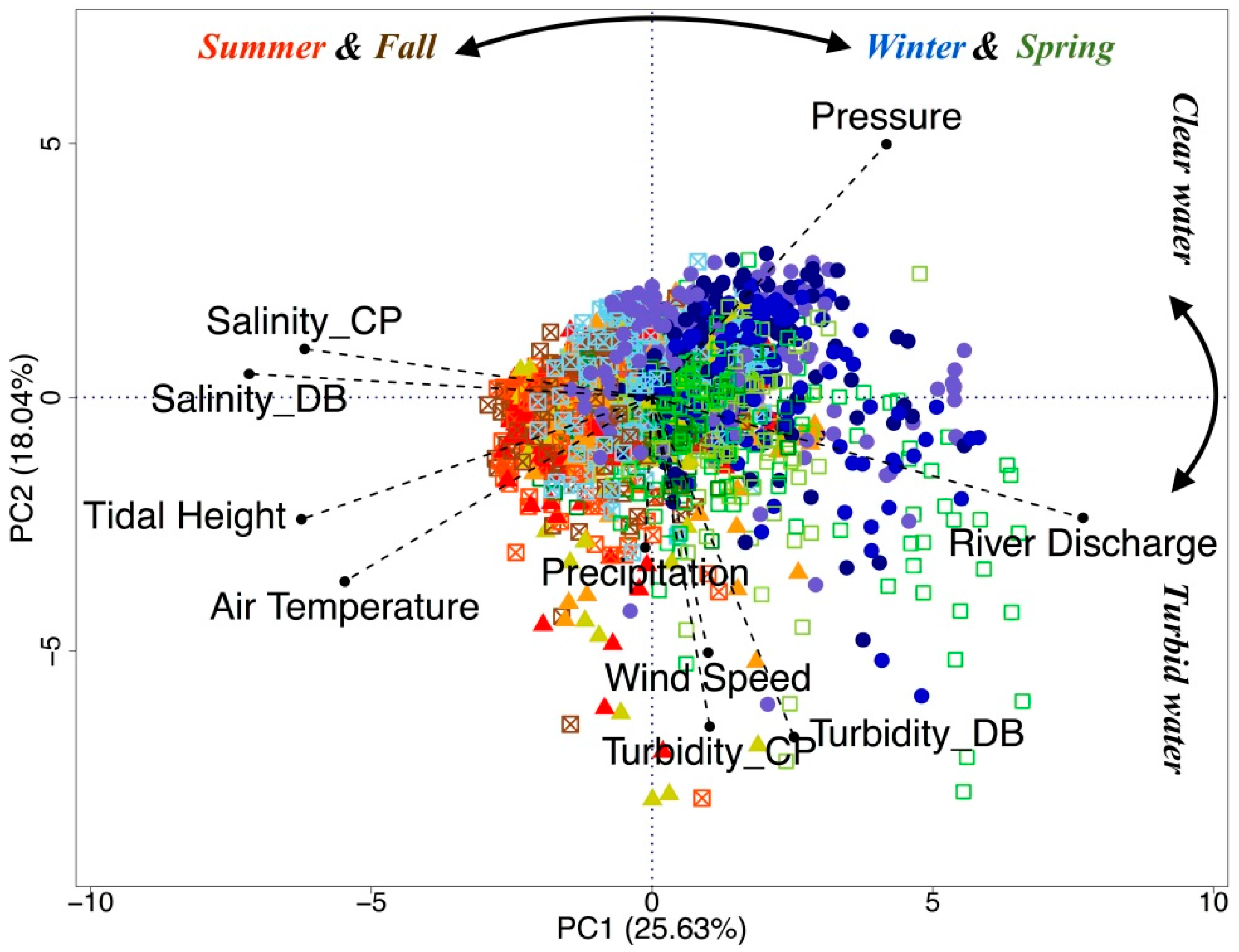
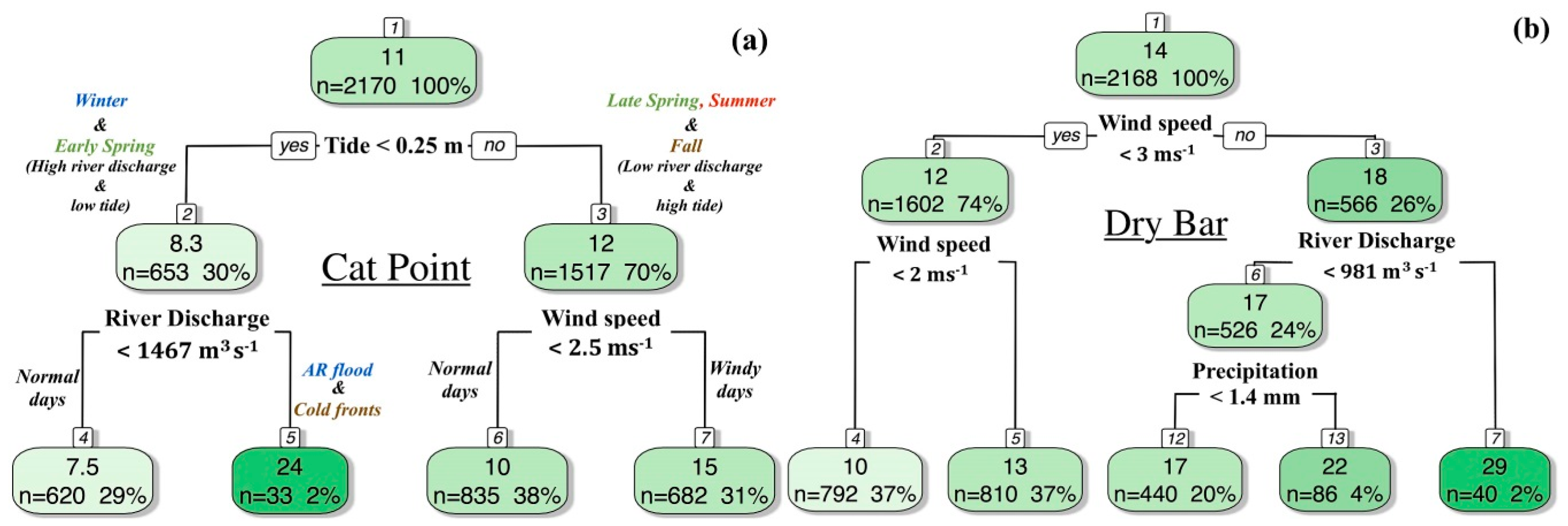

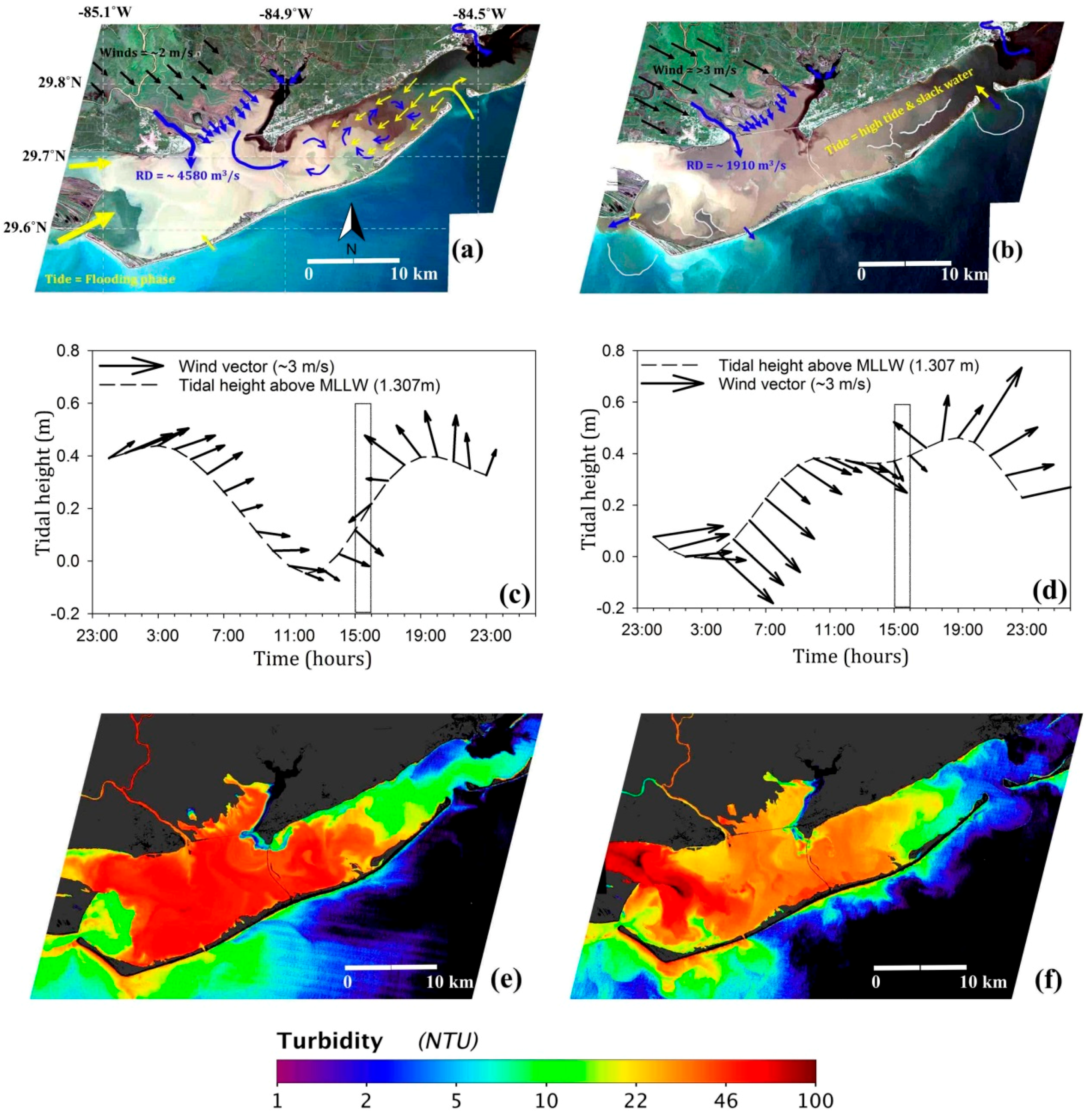
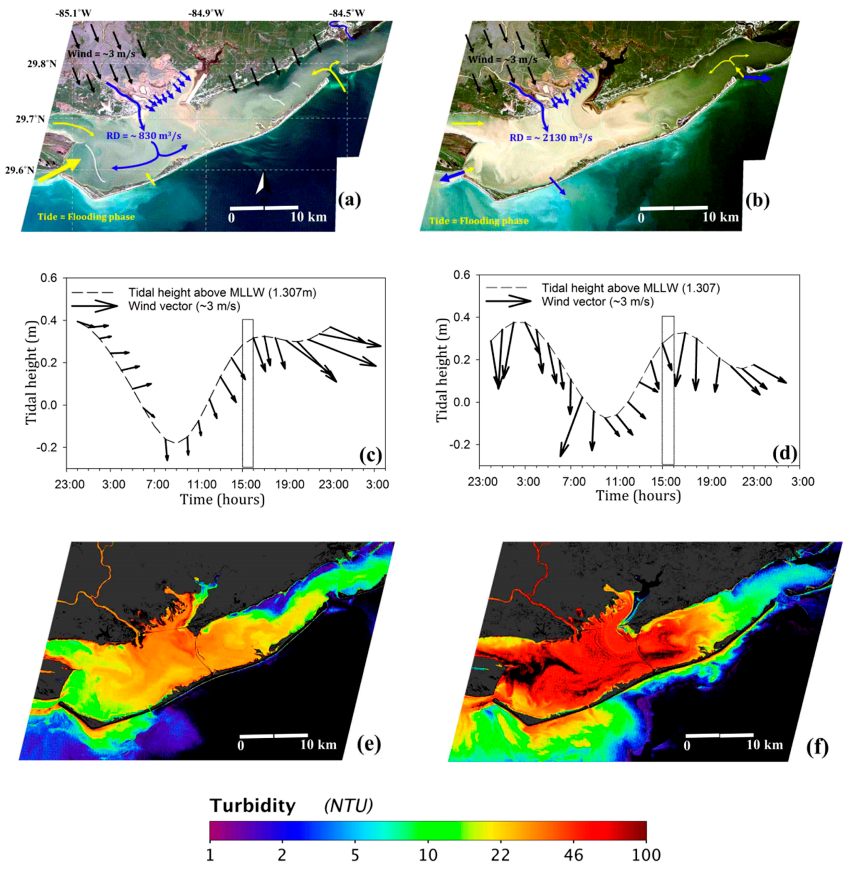
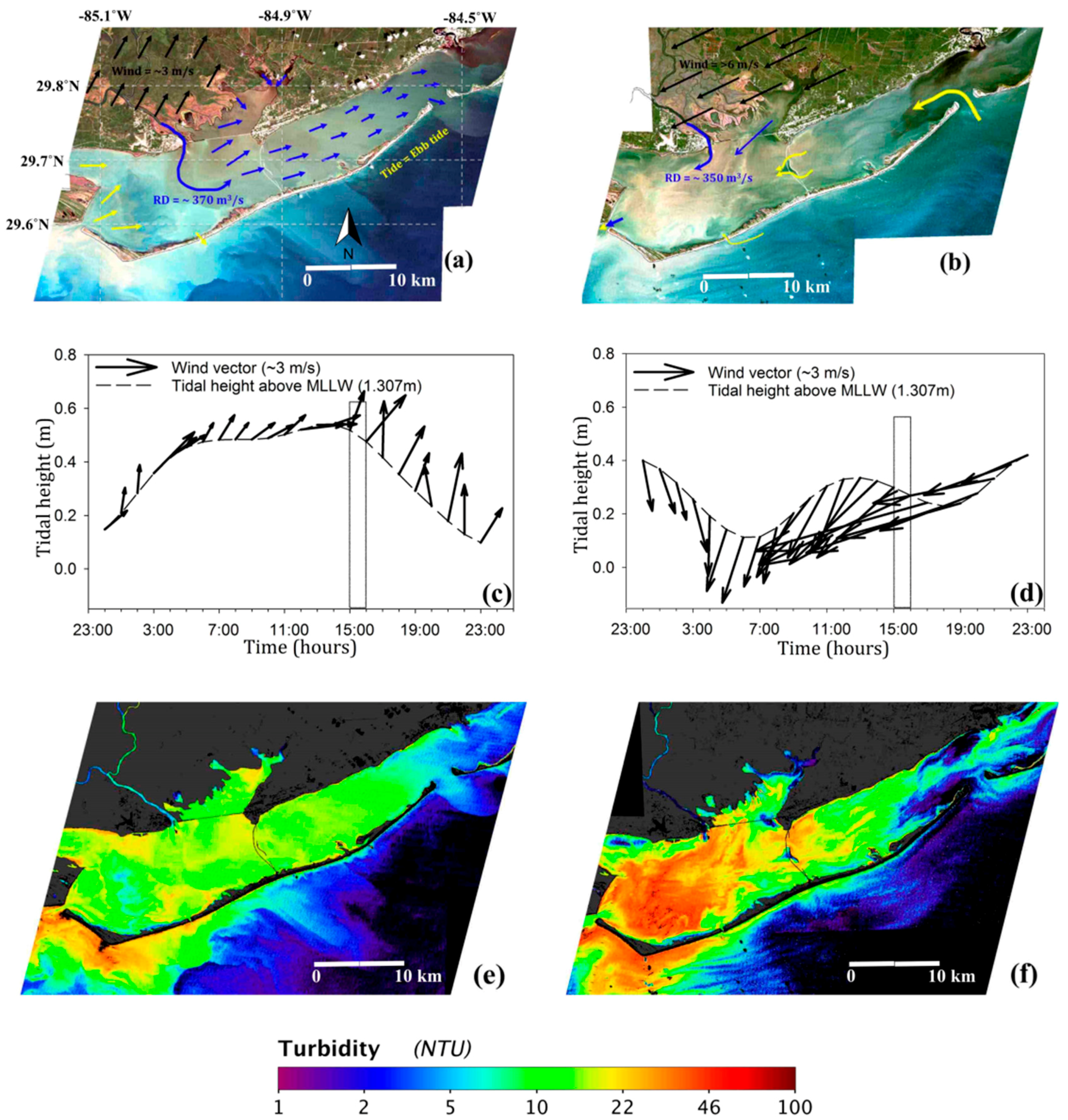

© 2017 by the authors. Licensee MDPI, Basel, Switzerland. This article is an open access article distributed under the terms and conditions of the Creative Commons Attribution (CC BY) license (http://creativecommons.org/licenses/by/4.0/).