Abstract
Knowledge of the exact statistical properties of the signal plays an important role in the applications of Polarimetric Synthetic Aperture Radar (PolSAR) data. In the last three decades, a considerable research effort has been devoted to finding accurate statistical models for PolSAR data, and a number of distributions have been proposed. In order to see the differences of various models and to make a comparison among them, a survey is provided in this paper. Texture models, which could capture the non-Gaussian behavior observed in high resolution data, and yet keep a compact mathematical form, are mainly explained. Probability density functions for the single look data and the multilook data are reviewed, as well as the advantages and applicable context of those models. As a summary, challenges in the area of statistical analysis of PolSAR data are also discussed.
1. Introduction
Synthetic Aperture Radar (SAR) and Polarimetric SAR (PolSAR) are widely used for observation of natural scenes. In most SAR or PolSAR systems, the size of a resolution cell is much larger than the wavelength. The measured signal is then a coherent addition of the echoes from all individual targets within that cell. Depending on the relative phases of each scattered wave, the coherent addition may be constructive or destructive, and it produces a salt-and-pepper appearance known as speckle over SAR images [1]. The target information, therefore, should be extracted through statistical analysis of the data. Hence, an accurate statistical model to describe the data becomes very important for the extraction of ground target properties [2,3,4,5,6].
Gaussian statistics for the radar returns have been frequently assumed when the spatial resolution of PolSAR images is moderate and the speckle is fully developed [1,7,8]. Actually, the number of targets in a resolution cell of low or medium resolution data is large. According to the Central Limit Theorem (CLT), Gaussian statistics could give a proper approximation to the data distribution. The Gaussian distribution is both mathematically tractable and efficient, making it very useful in specific applications. For SAR or PolSAR data, the mean value of the complex echo is generally assumed to be zero, and all the statistical properties are determined by the covariance matrix (or the coherency matrix) under the Gaussian assumption.
As the image resolution increases, analysis of real PolSAR data, however, reveals that non-Gaussian models give a more accurate representation of the data. The change of the observing surface could also give rise to non-Gaussian distributed data. Applications based on such models have better performance [2,4,9,10]. A common way to introduce non-Gaussianity is to divide the randomness of the radar images into two unrelated factors, texture and speckle. The texture models the natural spatial variation of the radar cross section, whereas the speckle, following a Gaussian distribution, conveys the polarimetric information. The texture and the speckle are incorporated with a product operation which leads to a doubly stochastic model called product model [11]. In the last two decades, a considerable research effort has been dedicated to investigate accurate product models for PolSAR data [12,13,14,15,16].
Another way to model the non-Gaussian behavior of PolSAR data is the so called finite mixture model [17,18,19], which assumes the data under analysis is a discrete mixture of different targets. This makes sense in certain scenes such as urban areas, which usually consist of coherent targets like houses and roads, as well as distributed targets like trees and grass. The backscattering from the urban area is a combination of different scattering mechanisms. It has been shown that for complex regions with irregular histograms, multimodal or spiky for example, the finite mixture model is more accurate than a single distribution [17].
As summarized in [20], there are many non-Gaussian distributions, including the Weibull distribution, the lognormal distribution, and the -stable distribution, suggested for the one-dimensional SAR data. However, these distributions are difficult to generalize to the multidimensional PolSAR data. A possible solution to this problem is to consider the idea of copulas [21]. First, we can use various non-Gaussian distributions to model the data of each polarimetric channel separately (called marginal distribution), and then introduce some common multivariate distributions to model the dependence of these marginal distributions. With the copulas, different marginal distributions and simple correlation structure can make up complex distributions for the PolSAR data [22,23].
As we can see, there are many statistical models proposed for the PolSAR data from different aspects. In this paper, a survey of these models is provided. PDFs for the single look data and the multilook data are mainly reviewed, as well as the advantages of those models. Analysis of real PolSAR data are performed using different statistical methods to evaluate the models.
The remainder of this paper is organized as follows. First, a few basic concepts of the polarimetric SAR are introduced, especially the notation employed in this paper. Then, statistics of the fully developed speckle will be discussed. Properties of the single look data and the multilook data are studied under the Gaussian assumption. The introduction of texture is followed, along with the widely studied texture models, including both the scalar texture models and the multi-texture models. Finally, finite mixture models as well as copula based models are detailed. Several experiments to validate applicability of different models are also given. Challenges in statistical modeling is summarized at the end.
2. Polarimetric SAR
PolSAR systems measure the properties of a distant target by detecting the change of the polarization state that the target induces to the incident wave. Let the polarized incident wave and scattered wave be expressed as the Jones Vectors [24]
where h represents the horizontal polarization state and v the vertical polarization state. It is possible to relate the incident and the scattered waves by means of a complex matrix [24]
where z is the distance between the target and the receiving antenna, and k is the wave number of the illuminating wave. The transformation matrix is generally referred to as scattering matrix and denoted by . It characterizes the target under observation with four complex-valued scattering coefficients. The diagonal elements of the scattering matrix receive the name “co-pol”, since they relate the same polarization for the incident and the scattered waves. The off-diagonal elements are known as “cross-pol” terms as they relate orthogonal polarization states [24].
The definition of depends on the coordinate systems. There are two principal conventions concerning the coordinate systems where the polarimetric scattering process can be considered: Forward Scattering Alignment (FSA) and Back Scattering Alignment (BSA) [24]. The difference lies in the way the coordinate system is selected to describe the polarization state of the scattered wave. The FSA is usually used when the transmitter and the receiver are not placed at the same spatial location, for example, for bistatic radar measurements. In contrast, the BSA is often adopted in monostatic radar measurements, in which the transmitting and receiving antennas are collocated in space. In this paper, we assume that the BSA convention is employed.
The interaction between the electromagnetic waves with a reciprocal medium follows the vector reciprocity theorem, which states that if we transmit a polarization state from position A, then the component polarized in the direction at position B is equal to the component of the scattered radiation when we illuminate the same object from B with polarization [25]. The reciprocity theorem applies to ground targets generally [25]. In the BSA coordinate system, the reciprocity theorem says that the cross-pol channels of the scattering matrix are equal, that is . Therefore, there are only three independent complex coefficients required to characterize the scatterer under observation.
In many cases, it is more flexible to represent the scattering matrix as a vector which is known as scattering vector. The vectorization can be performed through [26]
where is the matrix trace and is a complex matrix from a basis set which are constructed as an orthonormal set under the Hermitian inner product. The lexicographic basis and the Pauli basis are the most common ones in the context of radar polarimetry. The selection of the basis to vectorize the scattering matrix depends on the final purpose of the vectorization itself. When studying the statistical behavior of the PolSAR data, the lexicographic basis is more convenient due to its simplicity. The lexicographic basis set consists of the straightforward lexicographic ordering of the elements of the scattering matrix. For a reciprocal target, the scattering vector in this case can be expressed as
Targets under observation are commonly situated in a dynamically changing environment and are subjected to spatial and temporal variations. Despite the radar system transmits a perfectly polarized wave, the wave scattered by the target is partially polarized [25]. Such scatterers are called distributed targets. The analysis of this type of targets can not be performed exactly by one target but a population of targets. More precisely, they are analyzed by introducing the concept of space and time varying stochastic processes, where the targets are described by the second order moments such as the polarimetric coherency or covariance matrices.
The covariance matrix is defined as the expectation of the outer product of the target vector with its transpose conjugate
where and denote the transpose conjugate and conjugate, respectively. In practice, the number of scattering vectors used to calculate the expectation is limited. Let L denote the number of pixels to compute the average, the PolSAR data are then represented by the so-called sample covariance matrix
where is the ith scattering vector. The averaging is also called multilook processing which can be employed to reduce the speckle of PolSAR data, with L referring to the number of looks.
3. Gaussian Statistics
Under the assumption that the speckle is fully developed, it has been experimentally verified that the Gaussian statistics generally provide a good fit to SAR data, especially in homogeneous natural areas [7,27,28,29,30]. The multivariate Gaussian distribution, which is both mathematically tractable and efficient, is proper to model the scattering vectors when the surface roughness is relatively low, the spatial resolution is moderate, and a large number of scatterers are present [1,24]. The Gaussian assumption indicates that the statistical properties of the data are determined by the covariance matrix. The sample covariance matrix in this case follows a complex Wishart distribution, which is widely used in the applications of PolSAR data. There exist also some variations of the Wishart distribution that are shown to be more accurate in certain circumstances.
3.1. Gaussian Distribution
When a radar illuminates an area of a random surface containing many elementary scatterers, the scattering vector, , can be modeled as having a d-dimensional complex Gaussian distribution with zero mean. The Probability Density Function (PDF) is given by [31]
where is the determinant operation. The complex Gaussian distribution is denoted by for brevity. The real and imaginary parts of any complex element of are assumed to follow a circular Gaussian distribution. Consider the ith element for example, the joint PDF of the real and the imaginary parts can be written as
where . Let be the amplitude and be the phase of a complex value, then the real part of can be written as , and the imaginary part as . The Jacobian determinant of the transform from to is given by
Subsequently, the joint PDF of the amplitude and the phase can be obtained from (8) after changing variables, giving
The circular Gaussian assumption implies that the phase is uniformly distributed over , and independent from the amplitude. Averaging over the phase, therefore, gives the PDF of the amplitude
Equation (11) is known as the Rayleigh distribution, with mean value . The intensity of the ith channel, , can be easily proved to have a negative exponential distribution
with mean value and variance . This distribution shows that the useful information is described by a single degree of freedom, corresponding to the mean intensity.
Besides the intensity, the joint properties of two different polarimetric channels are of great interest. Considering two polarimetric channels and , the complex correlation coefficient is determined by
where and are, respectively, the amplitude and the phase of the complex correlation coefficient. The joint PDF of the real part and the imaginary part can be derived from (7), which is given as follows [30,32,33]
where , and . Write the complex values in the polar form, i.e., and , by changing variables from to , the previous distribution becomes
We are interested in the distributions of the product of the two amplitudes , and the phase difference , since their values reflect the correlation between different polarimetric channels. It can be shown that the Jacobian determinant of the transform from to is . Thus the following distribution can be obtained after changing variables
from which the joint PDF of z and can be further derived by integrating over and and employing the equality (A1)
Here is the modified Bessel function of the second kind of order v [34]. The marginal distribution of the product of the amplitudes, subsequently, is found to be
where is the modified Bessel function of the first kind [34] resulting from the integral identity (A2). Similarly, integrating (17) over the amplitudes and following the identity (A3) gives the marginal distribution of the phase difference
with . Note that is a complex number since is less than 1. Therefore, it can be represented in the polar form, e.g., , and as a result, (19) becomes
The PDFs shown in (18) and (20) can be also found in [32,33]. The Gaussian assumption implies that the statistics of the PolSAR data is completely determined by the covariance matrix. The properties described by the multivariate distribution (7) can be analyzed separately by the intensity (12), the product of amplitudes (18) and the phase difference (20).
3.2. Wishart Distribution
SAR data are frequently multilook processed for speckle reduction. Under the Gaussian assumption, the sample covariance matrix follows a complex Wishart distribution, , with PDF given by [31]
where the normalization factor is defined as
with referring to the gamma function. The Wishart distribution is valid only if . The random variables of this distribution are the diagonal terms of as well as the real and imaginary parts of the upper (or lower) off-diagonal terms. For a d-dimensional radar signal, the total number of independent variables is .
Considering only one polarimetric channel, from (21), we have the distribution of the intensity as
It is known as the gamma distribution with mean value and variance [35]. The number of looks can be estimated using the mean and the variance of the intensity
When L is equal to 1, the gamma distribution reduces to the exponential distribution (12). The variances of the two different distributions show that the multilook process reduces the speckle by scaling down the fluctuation magnitude with a factor .
For two polarimetric channels, saying channel i and channel k, the sample covariance matrix can be written as
Let represent the complex correlation coefficient, the joint distribution of , , and can be derived from (21), giving
where , , and . Write the off-diagonal element in the polar form, , by changing variables from to , the following result can be obtained
The determinant of must be greater than 0, therefore, we have . Integrating over using (A4) and then over using (A1) gives
Subsequently, the marginal distribution of the amplitude can be obtained following the integral identity (A2)
and the distribution of the phase difference by identity (A5)
where , and is the Gauss hypergeometric function [34]. Again, the statistical properties of the multilook data can be analyzed separately using (23), (29) and (30). The Wishart distribution is widely used in the modeling of PolSAR data [7,36,37,38], and there are several variations that make the model more accurate or efficient.
3.2.1. Relaxed Wishart Model
Compared with the multivariate complex Gaussian distribution, the Wishart distribution depends on an additional parameter, L, the number of looks. Assume that the multilook processing has different contributions to different types of targets, Anfinsen et al. proposed a refined model called relaxed Wishart distribution [39], in which the number of looks L is treated as a variable shape parameter. In other words, the number of looks is assumed to be distinct in different areas. It is observed that varying L gives a better representation of the data than using a constant L over all regions [39].
3.2.2. Wishart-Kotz Distribution
Another variation of the Wishart distribution is the Wishart-Kotz model [40,41], which exhibits the heavy tails needed to fit the data found in high resolution PolSAR images. In this model, there are no special mathematical functions involved that limit the usefulness by inflicting high computational cost and numerical instability. The sample covariance matrix in the Wishart-Kotz model is assumed to follow a Wishart-Kotz type I distribution with PDF defined as [40]
with additional parameters and , and a normalization constant factor c
Here is the same as that in Wishart model, see (22). The Wishart-Kotz distribution is a generalization of the Wishart distribution, which reduces to the latter when and .
4. Texture Model
The properties of the fully developed speckle are detailed in the previous section. This section illustrates how to model the texture statistically. There are two main manners to manage this: (1) consider the texture as a scalar random variable, or (2) consider it as a vector having the same dimension as the speckle component. They lead to the so called scalar texture model and multi-texture model, respectively. The texture random variable is generally assumed to be positive with unity mean. Therefore, it models the variation of the radar cross section only, leaving the intensities to the speckle component [7,42]. The statistical properties could be described by a certain distribution, or just a stochastic process without a specific PDF.
4.1. Scalar Texture Model
The scalar texture model assumes that the texture component in the product model is a positive scalar random variable. The scattering vector in this case can be written as [7,11,43,44]
where is the texture parameter with mean value equal to 1, and is the speckle vector, following a multivariate Gaussian distribution (7). The scalar texture model is also referred to as scale mixture of Gaussian [4], or Sphereically Invariant Random Vector (SIRV) [45,46,47]. For the multilook data, the sample covariance matrix can be expressed as
under the assumption that the texture has a higher spatial correlation than the speckle and the texture parameter is constant over the multilook processing window [13].
For a known , (33) implies that the scattering vector follows a complex Gaussian distribution (see Section 3.1) with PDF given by
And the distribution of the sample covariance matrix is given by
which is known as the Wishart distribution detailed in Section 3.2.
If the PDF of the texture random variable is not explicitly specified, can be viewed as an unknown deterministic parameter from pixel to pixel [47]. According to the concept of SIRV, an approximate maximum likelihood estimator for the texture parameter of each pixel is found to be [45,47]
where is the texture parameter of the ith pixel, d is the dimension of the target vector, and N is the number of pixels in the neighborhood. The estimators of the texture parameter and the covariance matrix depend on each other. They can be decoupled using a recursive process. Inserting into the second line of the above equation, the covariance matrix in the th iteration can be estimated by [45,46,47]
The process can be initialized by any matrix, even an identity matrix [47], and it is stopped when the Frobenius distance between two consecutive estimated matrices reaches some limit. More details about the existence as well as the convergence can be found in [46]. This estimator is referred to as fixed point estimator [47].
On the contrary, if the texture random variable is specified by a distribution, averaging all possible gives the unconditional or marginal PDF of the scattering vector
which is analytically solvable for some choices of . The PDF of the sample covariance matrix can be obtained similarly by
A number of models have been proposed in the literature by introducing different distributions for the texture component, including the distribution [13], the distribution [14,15], the Kummer- distribution [16], the , and the distribution [48], to represent different scenes of PolSAR data. They are explained in the following subsections.
4.1.1. Distribution
The distribution, assuming that the texture is gamma distributed, is widely used to model forests and the sea surface, and it can be unarguably regarded as one of the most successful radars models [4,10,12,13]. The gamma distribution is given by [35]
with shape parameter and scale parameter . The mean value is . Let to ensure the mean value of the texture is equal to 1, the distribution can be written as
4.1.2. Normal Inverse Gaussian (NIG)
The Normal Inverse Gaussian (NIG) distribution assumes that the texture follows an inverse Gaussian distribution [49,50]. The PDF of the inverse Gaussian distribution is given by
where is the mean value. By letting equal to 1 and replacing the random variable x with , the texture distribution becomes
Subsequently, the PDF of the scattering vector and the sample covariance matrix can be obtained by following the integral Equation (A1), giving
and
The NIG distribution has strong theoretical grounds derived from Brownian motion theory. Experiments demonstrate that it usually gives a better representation of the data than the Wishart distribution or the distribution does, because the inverse Gaussian distribution captures larger distribution shape variations than the gamma distribution [50]. In addition, the NIG distribution has less trouble at boundary mixtures than the distribution [50].
4.1.3. and Distributions
It is shown that the distribution and the distribution have a good representation of extremely heterogeneous regions such as urban areas [15]. Especially, the distribution has the same number of parameters as the distribution, but without complex special functions like the Bessel function which requires intensive computations [14,15].
The distribution assumes that the texture parameter obeys the Generalized Inverse Gaussian (GIG) law which is characterized by the PDF [14,51]
where , and p is a real parameter. The mean value of this distribution is . Letting gives
which can be further rewritten as follows by replacing with to reduce the number of parameters
Substituting (51) into (39) and (40), and calculating the integral using (A1) leads to
and
where . The above expressions are the PDFs of the scattering vector and the sample covariance matrix following distributions [14,52].
The distribution can be obtained from the distribution by letting . Representing the modified Bessel function using (A6), Equation (49) becomes
If , , , then after calculating the integral via (A7), the PDF of the GIG distribution is reduced to
Equation (55) is known as the inverse gamma distribution, or the reciprocal of the gamma distribution, with mean value . Let to ensure the mean value of the texture is equal to 1, the PDF becomes
The PDFs of the scattering vector and the sample covariance matrix of the distribution can be obtained by plugging the texture distribution into (39) and (40) respectively, and calculating the integral by (A9), giving
and
Another extreme case of the GIG distribution is the gamma distribution when , which leads to the distribution [14].
4.1.4. Kummer- Distribution
Assuming that the texture parameter follows a Fisher distribution, also known as the F-distribution or the Fisher-Snedecor distribution, with PDF given by [35]
where and , the scattering vector or the sample covariance matrix are Kummer- distributed, with the ability to model different types of textures, because the Fisher distribution covers a large range of distributions [16,53]. The mean value of the Fisher distribution is . Let to ensure the mean value of the texture variable equal to 1, we have the distribution for the texture as
Here parameters and are replaced by and to make the expression more concise. Inserting the texture distribution into (39), the PDF of the scattering vector can be calculated by
Replacing by , and using (A10) to calculate the integral results into the distribution of the scattering vector
where is the hyper-geometric function of the second kind [34]. By the same procedure, the distribution of the sample covariance matrix can be obtained as
As a matter of fact, Fisher distributions are the Pearson VI solutions and cover a large range of distributions. It is not only confined to urban scenes, but also fits reasonably in forest and agricultural fields [16,53]. The behavior of the head and tail of the distribution can be controlled by the two parameters and .
4.1.5. Distribution
The distribution assumes the texture to follow a beta distribution [48], which is given by [35]
The mean value of the beta distribution is . Let , , , the distribution of the normalized texture can be written as
The distribution of the scattering vector in this case can be calculated by
which leads to the following result according to the integral identity (A11)
where is Whittaker W function [34]. The distribution of the sample covariance matrix can be obtained by the same way
4.1.6. Distribution
Another possible distribution for the texture is the beta prime distribution, also known as inverted beta distribution, with PDF given by [35]
The mean value can be calculated by . Again, scale the random variable to ensure the mean value is equal to 1 by letting , the above distribution becomes
where the parameters are changed to , to make the expression brief. Equation (70) is the texture distribution of the distribution [48]. According to the product model, the distribution of the scattering vector can be calculated by
Employing the integral identity (A12), we have the PDF of the scattering vector as
and the PDF of the sample covariance matrix as
Here is the confluent hypergeometric function of the first kind, also known as the KummerM function [34]. The distribution and the distribution are able to model data with low variance but extreme skewness, which is particularly relevant to data with textural variability after a speckle filtering [48].
4.1.7. Wishart-Generalized Gamma Distribution
The Wishart-Generalized Gamma (WG) distribution employs the generalized gamma distribution to model the texture. The generalized gamma distribution has a more compact form and a larger variety of alternative distributions, with the gamma, the Weibull, the Rayleigh, and the exponential distributions being its special cases. Thus it is of greater flexibility in the statistical modelling [54]. The PDF of the generalized gamma distribution is given by [35]
which reduces to the gamma distribution (41) when . The mean value is given by . Scaling the mean value to 1, the PDF for the texture is obtained as
where . The distribution of the scattering vector then can be calculated by
There is no closed form expression for the above equation, but it can be solved numerically [54]. The distribution of the sample covariance matrix can be calculated by
It is reported that the WG distribution could provide better fitness than the and Kummer- distributions for different land cover types of homogeneous, heterogeneous, and extremely heterogeneous terrains [54].
4.1.8. Generalized Distribution
The well-known gamma distribution sometimes cannot fit the texture distribution accurately in very heterogeneous areas. In order to improve the flexibility of the model, it is assumed that the texture follows a Laguerre expansion of the gamma distribution [55], with its PDF given by
where , the mean value, is normally assumed to be equal to 1, and
The Laguerre polynomial is given by
The PDF of the sample covariance matrix in this case can be expressed as [55]
which is a weighted combination of a series of distributions based on a Laguerre polynomial expansion. It shows that the generalized distribution gives a better approximation than the distribution when there exist strong scatterers in the scene [55].
4.2. Multi-Texture Model
In the scalar texture model, different polarimetric channels are assumed to have a common texture variable. However, if the electromagnetic wave sees different geometrical or dielectric properties of the target, and if those properties are spatially modulated, then the texture of each channel should be different [56]. For example, in scattering from forest areas, volume scattering will affect the cross-pol component stronger than the co-pol channels, whereas surface scattering will have the opposite effect [57]. The scalar texture model must, therefore, be extended to take into consideration the different radar cross section modulations in polarimetric channels. One solution is to allow for a vector component of the texture in the product model. This type of models are called multi-texture models.
Under the assumption of reciprocity, there are only three independent complex coefficients required to characterize the scatterer under observation. The multi-texture model then can be formulated as [57,58,59,60]
where represents the speckle, following a multivariate Gaussian distribution (see Section 3.1), and is a diagonal matrix containing texture variables for each channel
The texture parameters are assumed to be positive, and we have equal to , the identity matrix. Assuming that the texture variables are constant on the scale of the multilook processing window, the sample covariance matrix can be written as
where is Wishart distributed, see Section 3.2.
Provided that the distributions of the texture variables are known, the PDF of the scattering vector can be calculated using
where is the set of all diagonal matrices with non-negative entries. After changing variable by , the conditional distribution of on can be obtained from (7), giving
By the similar way, we have the distribution of the sample covariance matrix as [57,59]
where
Different texture variables for the multi-texture model can be: (1) totally dependent, in which case it reduces to the scalar texture model, (2) independent from each other, that is, texture variables follow different distributions with different parameters, or (3) partially correlated [58,61]. In many cases, it is reasonable to assume co-pol channels have the same texture but different from that of the cross-pol channels. This type of models is usually referred to as dual-texture model [57,59,62]. For reciprocal media with reflection symmetry for example, the PDF of the sample covariance matrix can be expanded as [59]
where and denote the th entry of matrix and respectively. The texture of the co-pol channels is represented by and that of the cross-pol channel by .
4.2.1. Correlated Distribution
The correlated distribution assumes that the texture variables of different polarimetric channels are partially correlated, each following a gamma distribution [58,61]. Unfortunately, there is no explicit expression for the joint distribution of the texture variables, or the correlated gamma distribution. In this model, the texture of polarimetric channel i, specified by the PDF (42) with parameter , is given by [61]
where is the ith element of the vector , which is Gaussian distributed with zero mean, variance one, and correlation matrix . The correlation properties of the texture variables is also specified by . The characteristic function of the vector containing all texture variables is [61]
where is a diagonal matrix having the entry equal to the ith element of the characteristic function variable . This model requires that all polarimetric channels have the same half-integer distribution parameter , e.g., 0.5, 1.5, 2.5 and so on.
4.2.2. Dual-Texture Distribution
The dual-texture distribution is derived by considering different texture variables for co-pol and cross-pol channels. Both the co-pol and the cross-pol texture variables are modelled by the GIG distributions (49), which yields a more flexible multivariate distribution [62]. Under the assumption of reciprocity and reflection symmetry, the statistical properties of the single look complex data is characterized by the distribution [62]
where consists of all parameters for the GIG texture distributions (see Section 4.1.3), , and , with and indexing entries of and respectively.
5. Other Models
To model a complex scene using texture models, we often need to introduce complicated distributions with many parameters to describe the statistical behavior of the texture component. However, having more parameters requires a more complicated estimation process by considering higher order statistics. In addition, higher order moment estimators are known to have higher variance. With the limited sample sizes used in the modelling, such complicated modelling may be very inefficient [50]. To overcome this problem, some researchers try to divide a complex model into multiple simple components and then find a way to combine these components together. The finite mixture model and copula based model detailed as follows are based on this idea.
5.1. Finite Mixture Model
The heterogeneity that appears in PolSAR data may result from the mixture of different targets. For instance, from an urban area which usually consists of different objects like houses, trees and roads, the backscattering is a combination of different scattering mechanisms. The forest areas sometimes can be treated as a mixture of bright clutters and dark ones, corresponding to the strong returns from the crowns of trees and the shadows behind them. To represent this type of data, a simple model would be inappropriate. Finite mixture models, instead, could achieve reasonable level of accuracy [17,18,19,63,64].
Assume that the region under analysis can be modeled by a mixture of K components, then the overall PDF of the data can be written as a weighted sum of the probabilities of each component [65]
where is a vector containing all the parameters of the distribution and the mixing proportions obey
It has been shown that for complicated regions with more irregular histograms (multimodal, spiky), the finite mixture model is more accurate than a single distribution [17,18,19].
There are many options for the distributions of the mixing components, but here we mainly focus on the mixture of Wishart distributed components. For different mixing components, the number of looks are the same. The PDF, therefore, can be written as
where and is given by (22). The PDF of the ith channel intensity, which is also a finite mixture, is found to be
where . The most interesting property of a mixture density is that the shape of the density is extremely flexible. A mixture density may be multimodal, or even if it is unimodal, may exhibit considerable skewness or additional humps. For this reason, finite mixture distributions offer a flexible way to describe rather heterogeneous data by summarizing the characteristics of the data in terms of the number and the spread of the mixture components [65].
5.2. Copula Based Model
Copulas are popular in high-dimensional statistical applications as they allow one to easily model and estimate the distribution of random vectors by estimating marginals and dependence separately [21]. They are of great interest for two main reasons: (1) as a way to study scale-free measures of dependence; and (2) as a starting point for constructing families of multivariate distributions [21]. For the PolSAR data, we often have a much better idea about the marginal behaviour of individual polarimetric channels than we do about their dependence structure. The copula approach allows us to combine our more developed marginal models with a variety of possible dependence models to investigate the statistical behavior of the data.
A d-dimensional copula, denoted by , is a joint Cumulative Distribution Function (CDF) of a d-dimensional random vector on the unit hypercube with uniform marginals. More specifically, a copula is a function C from to with the following properties [21,66]:
- , the copula is equal to 0 if at least one parameter is 0.
- , the copula is equal to if all parameters are 1 except .
- For each hyperrectangle where , the C-volume of B is non-negativewhere represents the corners of the hyperrectangle, and is the number of elements in reaching the lower bound of the hyperrectangle.
According to Sklar’s Theorem, any multivariate joint distribution can be written in terms of univariate marginal distribution functions and a copula which describes the dependence structure between the variables [21]
where is the continuous marginal CDF . The copula C contains all information about the dependence structure whereas the marginal cumulative distribution functions contains all information about an individual random variable.
There are many parametric copula families available, which usually have one or more parameters controlling the strength of dependence. The most popular ones include the elliptical copulas (such as the Gaussian copula and the student t copula), and the Archimedian copulas. In the context of PolSAR data modeling, the Ali-Mikhail-Haq copula which belongs to the Archimedian family is demonstrated to be appropriate [22,23,67]. The Gaussian copula is also found to be proper to model the wavelet coefficients [68]. Though it is a hot topic, the study of copulas and the role they play in statistics and stochastic processes is a subject still in its infancy. There are many open problems and much work to be done.
6. Model Analysis
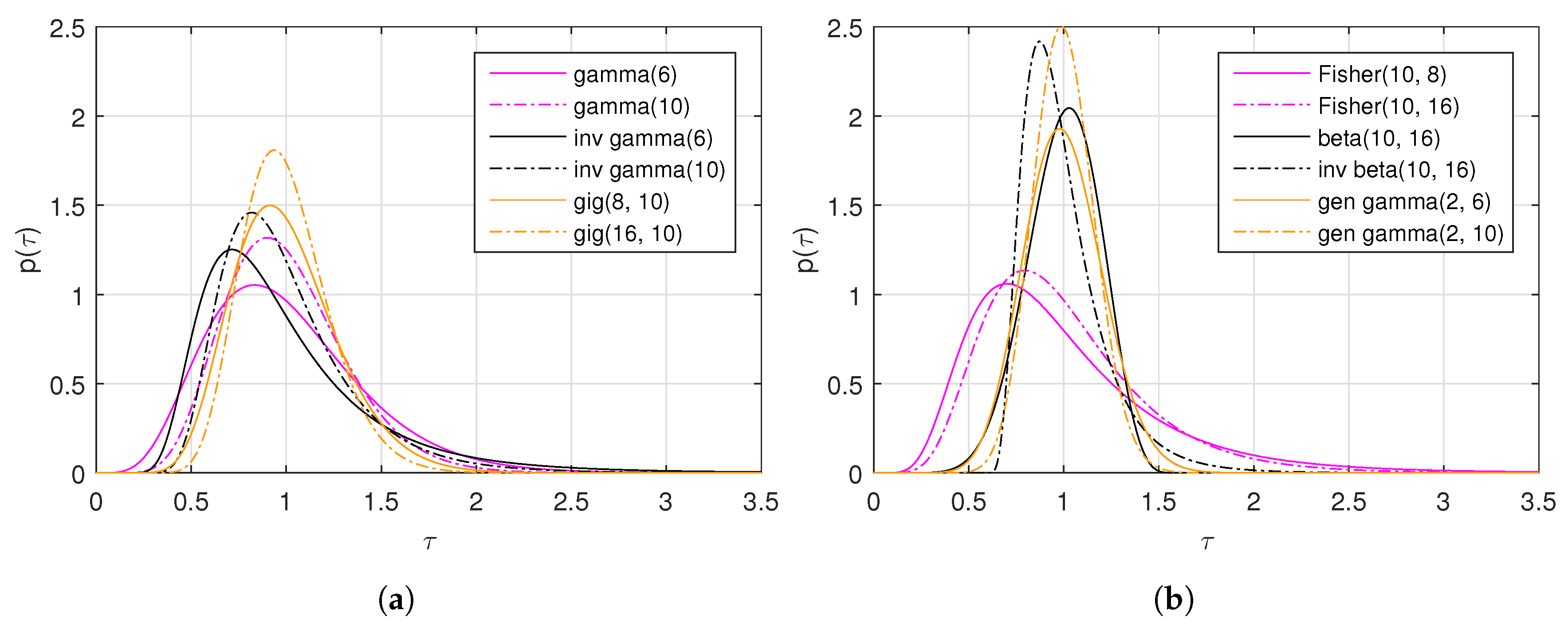
In the previous sections, the statistical models proposed for the PolSAR data are reviewed, with an emphasis on the derivation of PDFs for the scattering vector and the sample covariance matrix. The models are categorized into three groups: (1) Gaussian Models, (2) Texture Models, and (3) The Others. Table 1 shows a summary of all these models. As we can see, texture models are still the main focus in statistical modeling of PolSAR data. Several examples of the texture distributions with different distribution parameters are plotted in Figure 1.

Table 1.
Summary of statistical PolSAR data models.
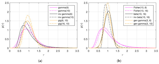
Figure 1.
Examples of different texture distributions. (a) PDFs of the gamma (gamma(6) and gamma(10)), the inverse gamma (inv gamma(6) and inv gamma(10)) and the GIG (gig(8, 10) and gig(16, 10)) distributions. (b) PDFs of the Fisher (Fisher(10, 8) and Fisher(10, 16)), the beta (beta(10, 16)), the inverted beta (inv beta(10, 16)), and the generalized gamma (gen gamma(2, 6) and gen gamma(2, 10)) distributions.
In the remaining of this section, we will show some experimental results on the applicability of different statistical models.
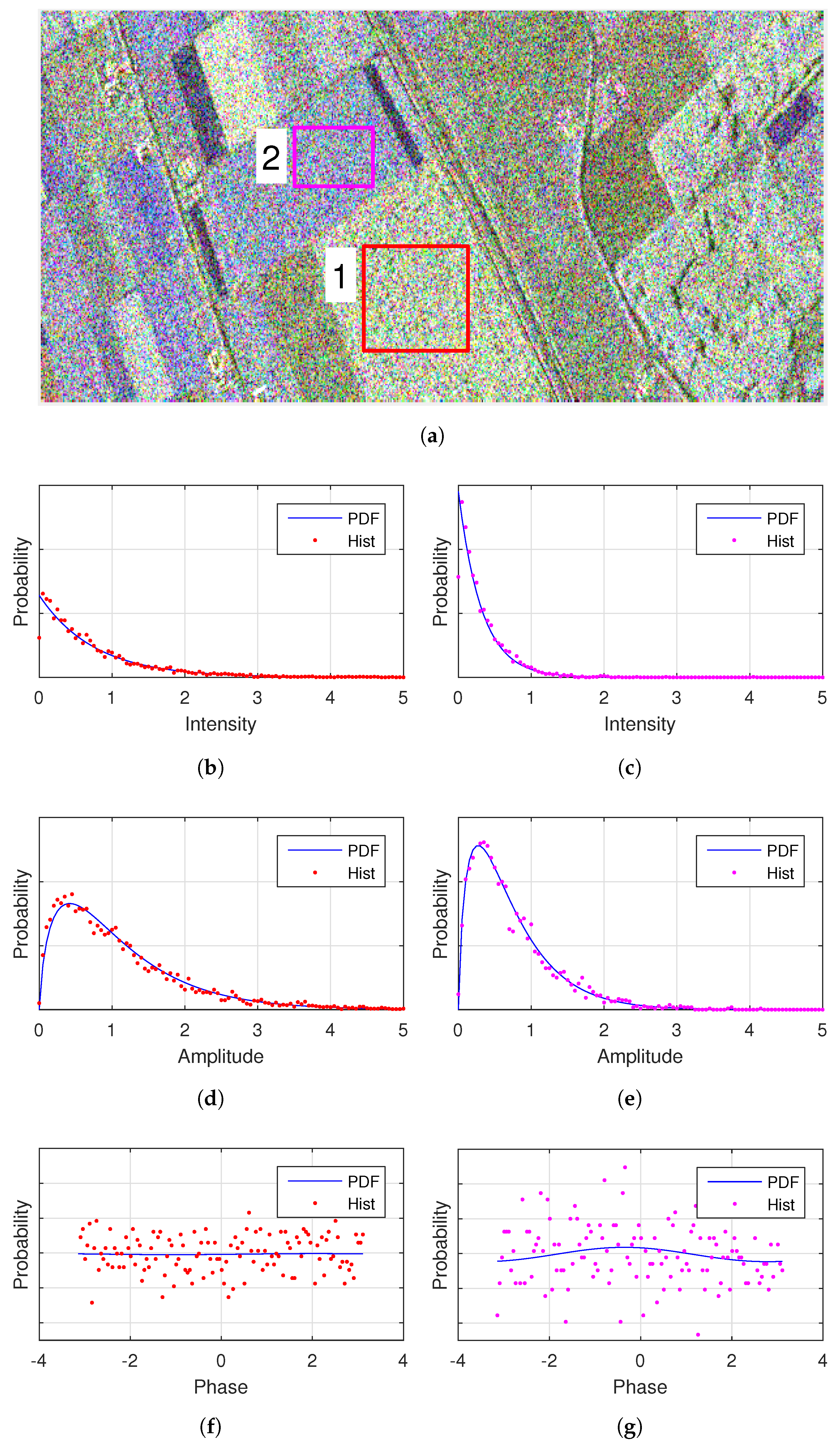
First of all, two homogeneous Regions Of Interest (ROI) over the farmland of a RADARSAT-2 image are analyzed, as shown in Figure 2. The data, in single look complex format, has a spatial resolution of 11.1 m × 7.6 m (Range × Azimuth). It was acquired over Flevoland (The Netherlands) with the Fine Quad-Pol mode during the ESA-led AgriSAR 2009 campaign. Statistical properties are analyzed separately by the histograms of the intensity, the product of amplitudes and the phase difference between two polarimetric channels. To tell whether Gaussian distributions are proper or not, the histograms are compared with the PDFs defined by (12), (18) and (20). The covariance matrices of the Gaussian distributions are estimated using the simple mean estimator.
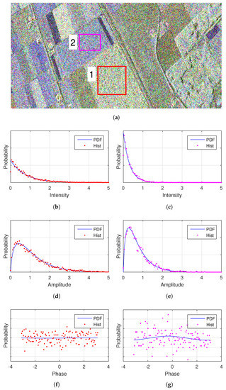
Figure 2.
Histograms of two homogeneous areas in a RADARSAT-2 image and the PDFs under Gaussian assumption. Parameters of the Gaussian distributions are estimated using moments. (a) Pauli decomposition of the RADARSAT-2 data and two ROIs. (b,c) Intensity of the . (d,e) Amplitude of . (f,g) Phase of .
Figure 2 shows the fit of the HH intensity, and the fit of the product of HH Channel and HV channel. It demonstrates that the histograms conform to the corresponding PDFs, implying that Gaussian distributions are suitable for these crops areas. Though it could work, the comparison of histogram and PDF is not visually effective, see Figure 2f,g for example. So in the next experiments we will try different methods to validate the applicability of statistical models.
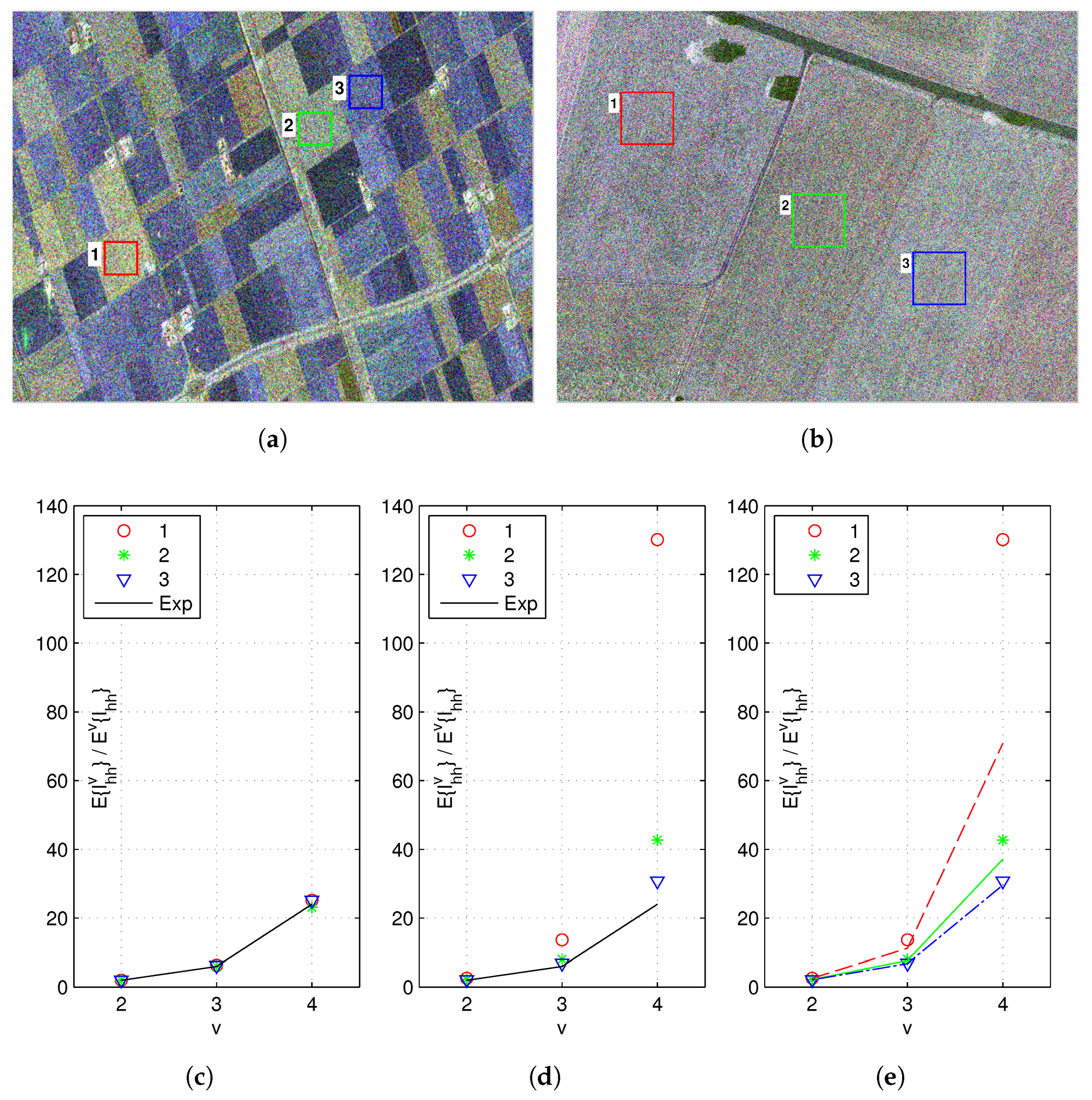
As mentioned in the previous sections, the spatial resolution of PolSAR images is one of the most important factors that have strong impact on the data statistics. To demonstrate this, real SAR data including a RADARSAT-2 Fine Quad-Pol data (RST2) as well as a F-SAR X-band full-pol data (FSAR) are analyzed. The two data have quite different spatial resolutions, 11.1 m × 7.6 m for the RST2 data, and 0.25 m × 0.25 m for the FSAR data. Three ROIs over the crops area from each data are tested, see Figure 3a,b. For the RST2 data, each ROI covers pixels. The ROIs in the FSAR data are much larger thanks to a higher spatial resolution, each covering pixels. The Pauli decomposition shows that the ROIs in both images are very homogeneous, no appreciable texture is observed.
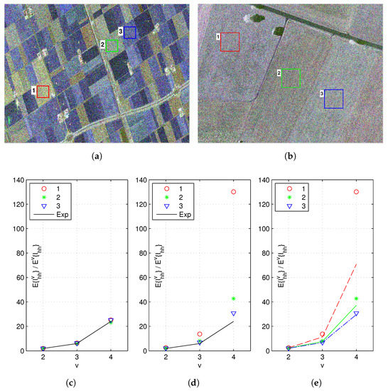
Figure 3.
NIMs of the 2nd, the 3rd and the 4th order estimated from three crops areas in a RADARSAT-2 data and a F-SAR data. (a) Pauli decomposition and ROIs of the RADARSAT-2 image. (b) Pauli decomposition and ROIs of the F-SAR image. (c) NIMs of the ROIs in the RADARSAT-2 data and the exponential distribution. (d) NIMs of the ROIs in the F-SAR data and the exponential distribution. (e) NIMs of the ROIs in the F-SAR data and Weibull distributions.
Normalized Intensity Moments (NIM) are employed to determine whether the Gaussian distributions are suitable for the test ROIs or not [9,69]. Let I denote the intensity of a polarimetric channel, the NIM of the vth order is defined as
For Gaussian distributed data, the intensity will follow an exponential distribution as defined in (12). The NIMs in this case are independent of the data, which can be calculated by
By comparing the estimated values from the data with those of Gaussian distributions, we can easily make conclusions on the applicability of Gaussian distributions.
The HH channel is analyzed for both the RST2 data and the FSAR data. Results are shown in Figure 3c,d, where black lines represent theoretical values of the exponential distribution and different markers represent values estimated from the test ROIs. As it can be seen, the NIMs estimated from the RST2 data fit those calculated from the exponential distribution very well. Same results can be obtained for the HV channel and the VV channel. It is rational to conclude that these ROIs can be modeled by Gaussian distributions. In contrast, the result on the FSAR data shows different behaviors. There are large discrepancies between the estimated values and the theoretical values for all ROIs. Apparently, Gaussian distributions are not accurate any more.
A further validation on the FSAR data is performed. Assuming that the intensity of each ROI can be modeled by a Weibull distribution, then the distribution parameter, denoted by , can be estimated using the first order moment. Furthermore, the NIM of the vth order can be computed by
In Figure 3e, the estimated NIMs (markers) and those calculated using the above equation (lines) are plotted for each ROI. The Weibull distribution seems to be applicable in ROI 2 and ROI 3. Compared with the exponential distribution, the Weibull distribution could capture larger variance by introducing an additional distribution parameter. However, even the Weibull distribution could not give an accurate representation for ROI 1. Complex distributions with more parameters may achieve reasonable fit.
In general, the Weibull distribution is advisable to model the intensity of high resolution single channel data. However, for PolSAR data, the correlations between different polarimetric channels convey useful information, besides the intensities. In order to describe the statistical behavior correctly, copulas (introduced in Section 5.2) can be adopted. By modeling the dependence structure between polarimetric channels using copulas, and the intensities by Weibull distributions, a good approximation of the data could be expected. However, how to choose the proper copulas needs to be investigated intensively. We haven’t found a copula capturing the dependency properly for the testing ROIs.
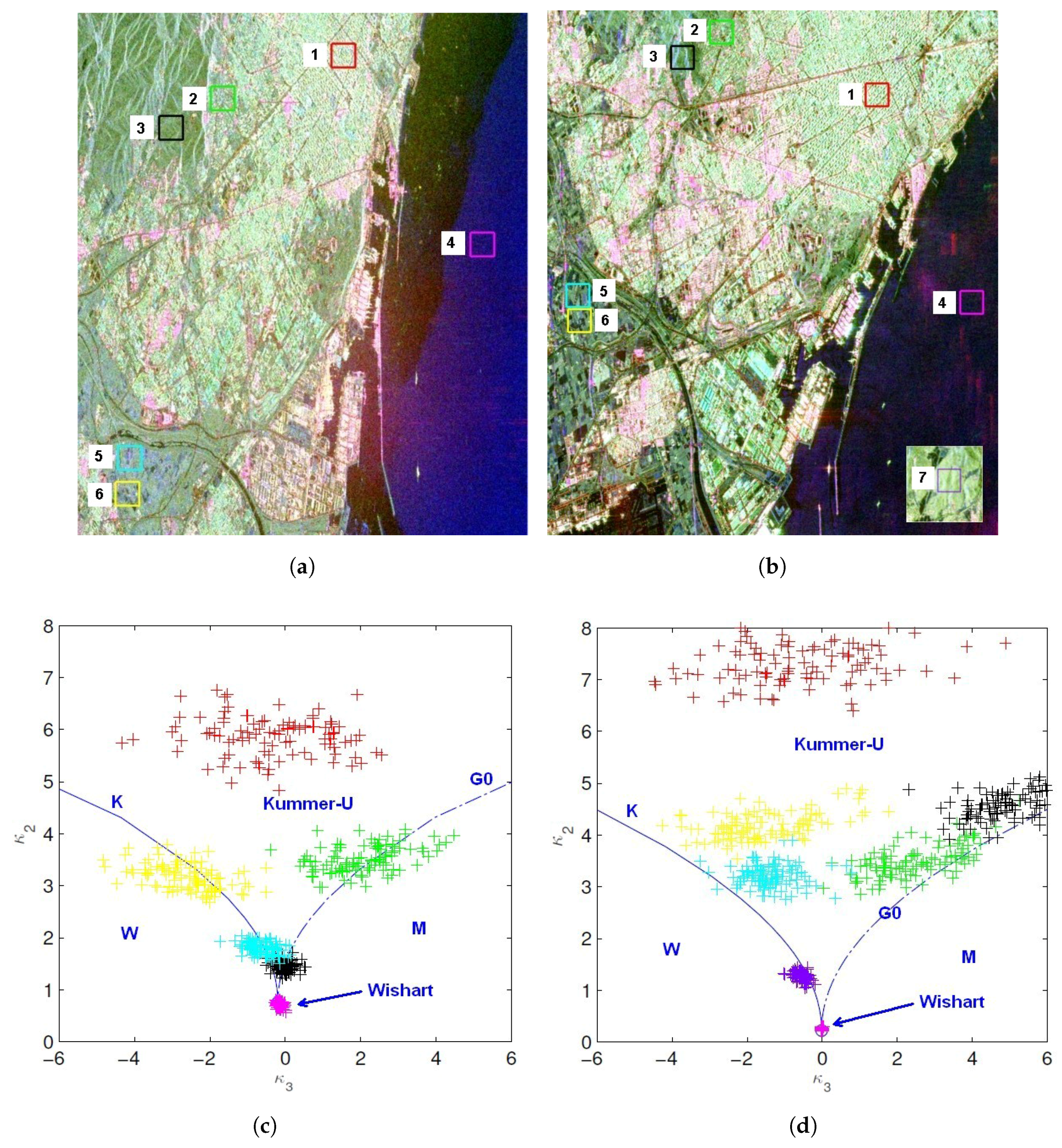
Another aspect that causes non-gaussianity in PolSAR data is the fluctuation of radar cross section due to the change of surface properties, e.g., height of the observing surface. Usually, this type of data should be modeled using texture distributions. To validate the applicability of texture models, two PolSAR images, the RADARSAT-2 Fine Quad-Pol data (RST2) and the ALOS-2 level 1.1 Full-Pol data (ALOS2), are analyzed. Both images were acquired over Barcelona (Spain) with similar incidence angles. The spatial resolution is different, 11.1 m × 7.6 m (Range × Azimuth) for the RST2 data and 3.49 m × 3.84 m for the ALOS2 data, respectively. Original data are in the single look complex format, from which the sample covariance matrices are obtained after applying a multilook processing. We have selected ROIs locating at similar positions in the urban area, in the agriculture area, in the sea and the forest areas. Pauli decomposition of the test data and ROIs are shown in Figure 4.

Figure 4.
Matrix variate log-cumulants of the 2nd and the 3rd order estimated from a RADARSAT-2 data and an ALOS-2 data. Theoretical values calculated from the , the , the Kummer-, the , the and the Wishart distributions are also plotted as references. (a) ROIs of the RADARSAT-2 data. (b) ROIs of the ALOS-2 data. (c) Matrix variate log-cumulants of the RADARSAT-2 data. (d) Matrix variate log-cumulants of the ALOS-2 data.
Matrix variate log-cumulants [42] are used to examine the suitability of texture models. The matrix variate log-cumulants are of great value for the analysis of sample covariance matrix, and that they can be employed to derive estimators for the distribution parameters with low bias and variance [42]. Different from the NIMs, there is no need to study each polarimetric channel separately with matrix variate log-cumulants. Define the Mellin kind matrix-variate characteristic function as the Mellin Transform of the PDF
then, the vth-order log-cumulant, or Mellin kind cumulant, is given by
Meanwhile, the sample log-cumulants can be estimated from the data using
where is the estimated log-moments
with M denoting the number of samples and the ith sample covariance matrix.
To see if a texture model is applicable, we can compare the log-cumulants calculated from the PDF () and those estimated from the sample data (). In [42], a diagram is proposed to visualize the comparison by plotting the second order log-cumulants against the third order log-cumulants in a plane, where different distributions place in different regions, as shown in Figure 4c,d. In this diagram, estimated log-cumulants are represented by the "+" markers (values from different ROIs are distinguished by various colors), and theoretical values of different texture distributions are represented by curves (the and the distributions) as well as regions (the Kummer-, the and the distributions).
From Figure 4, we can see that the urban areas (red and green rectangles) can be modeled by the or the Kummer- distributions, which have the capability to model heterogeneous areas. The two ROIs in urban area represent two different urban structures, one is of tall and densely distributed apartments, the other is of short and sparse houses. This may be an explanation as to why different statistics, the vs the Kummer-, are obtained. In agriculture areas (cyan and yellow rectangles), distribution is shown to be the most suitable model. The forest area (black rectangle) shows weak texture in the RST2 data. In the ALOS2 data, there is a strong fluctuation in the backscattering due to the radar foreshortening. To eliminate the effect of radar image distortions, another forest region (purple rectangle) is analyzed, which is found to follow a distribution. In most cases, texture is not observed in the sea areas.
As explained in Section 5.1, the finite mixtures could also give rise to non-gaussian statistics. To further distinguish textures from mixtures, higher order log-cumulants are required [70]. A large number of samples are demanded in order to estimate the higher order log-cumulants correctly. There are only pixels in each of the previous ROIs, not enough to obtain a satisfying estimation of the fourth order log-cumulants. So another experiment is carried out on an airborne SAR data, a UAVSAR image.
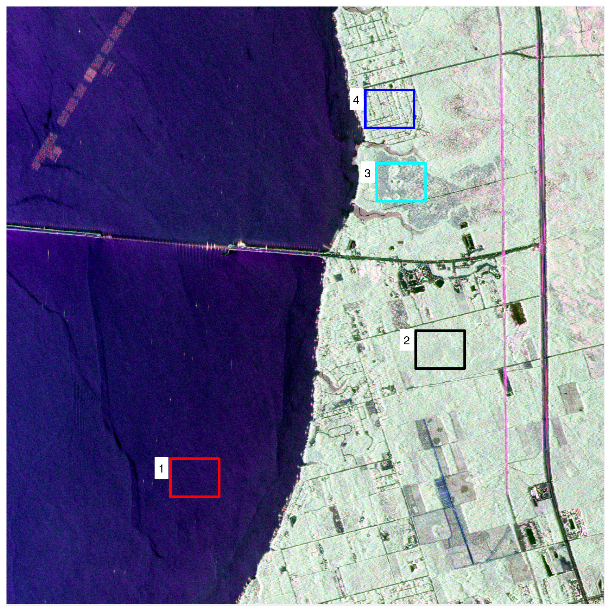
The test site is in the West Panhandle of Florida (USA), and the data is in the multilook cross-product slant range format, with number of looks in the range dimension and azimuth dimension equal to 3 and 12 respectively. The ENL is estimated as 12.73 over a homogeneous sea area. Four ROIs covering land types of ocean area (ROI 1), forest (ROI 2), wetland (ROI 3), and urban area (ROI 4), are tested, see Figure 5. Thanks to a higher spatial resolution, 1.67 m × 0.8 m (Range × Azimuth), each ROI contains pixels, much more samples than those in the previous experiment.
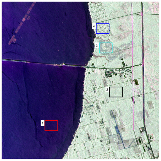
Figure 5.
Test regions on the UAVSAR data. Four ROIs over different land types are tested, including the sea, the forest, the wetland and the urban area.
The log-cumulants of the second order, the third order and the fourth order are calculated. From the log-cumulant diagrams (Figure 6a,b), we can see that different ROIs show different statistical behaviors. The ocean area can be modeled by a Wishart distribution, and the forest by a distribution. The wetland and the urban area are very heterogeneous, especially the urban area, which has a very small . The point clouds representing estimated statistics are less widely spread than those in Figure 4c,d. This is because more samples are used to estimate the values.
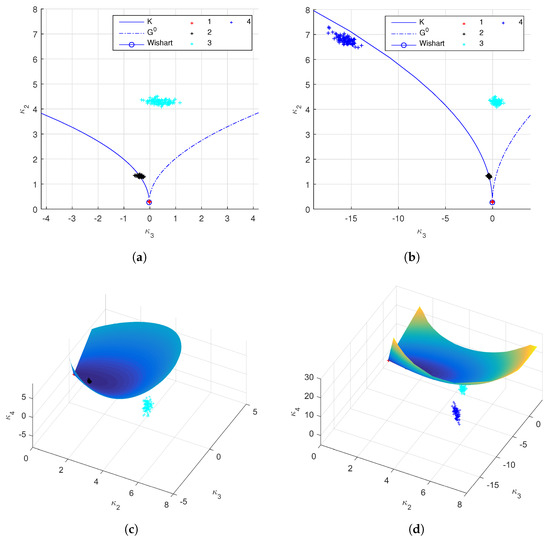
Figure 6.
Log-cumulants of the 2nd, the 3rd and the 4th orders on the UAVSAR data. The right column and the left column are the same results but with different axes limits. (a,b) Log-cumulants of the 2nd and the 3rd order. ROIs over different ground targets show different statistics. (c,d) Log-cumulant up to the 4th order. It shows some ROIs can be modeled by texture models, while others should be represented using finite mixture model.
The fourth order log-cumulant is considered to further discriminate the texture from mixture. As shown in Figure 6c,d, the log-cumulants of major texture models can construct a smooth surface, while those of the finite mixture model will lie below this surface. The results show that texture models are proper for the sea area and forest area, while a finite mixture model make a better representation than a texture model for the wetland area and the urban area, because the point clouds estimated from ROI 1 and ROI 2 are on the product model surface, whereas those from ROI 3 and ROI 4 are below it. Actually, the Pauli decomposition in Figure 5 shows that the first two ROIs are very homogeneous and ROI 3 consists of different targets. Urban area, made up of distributed targets and point targets usually, has very large variance. This can be verified by the log-cumulant cube in Figure 6d, where both of the absolute values of and are very large. The estimation of the number as well as the weights of mixing components needs to be further studied.
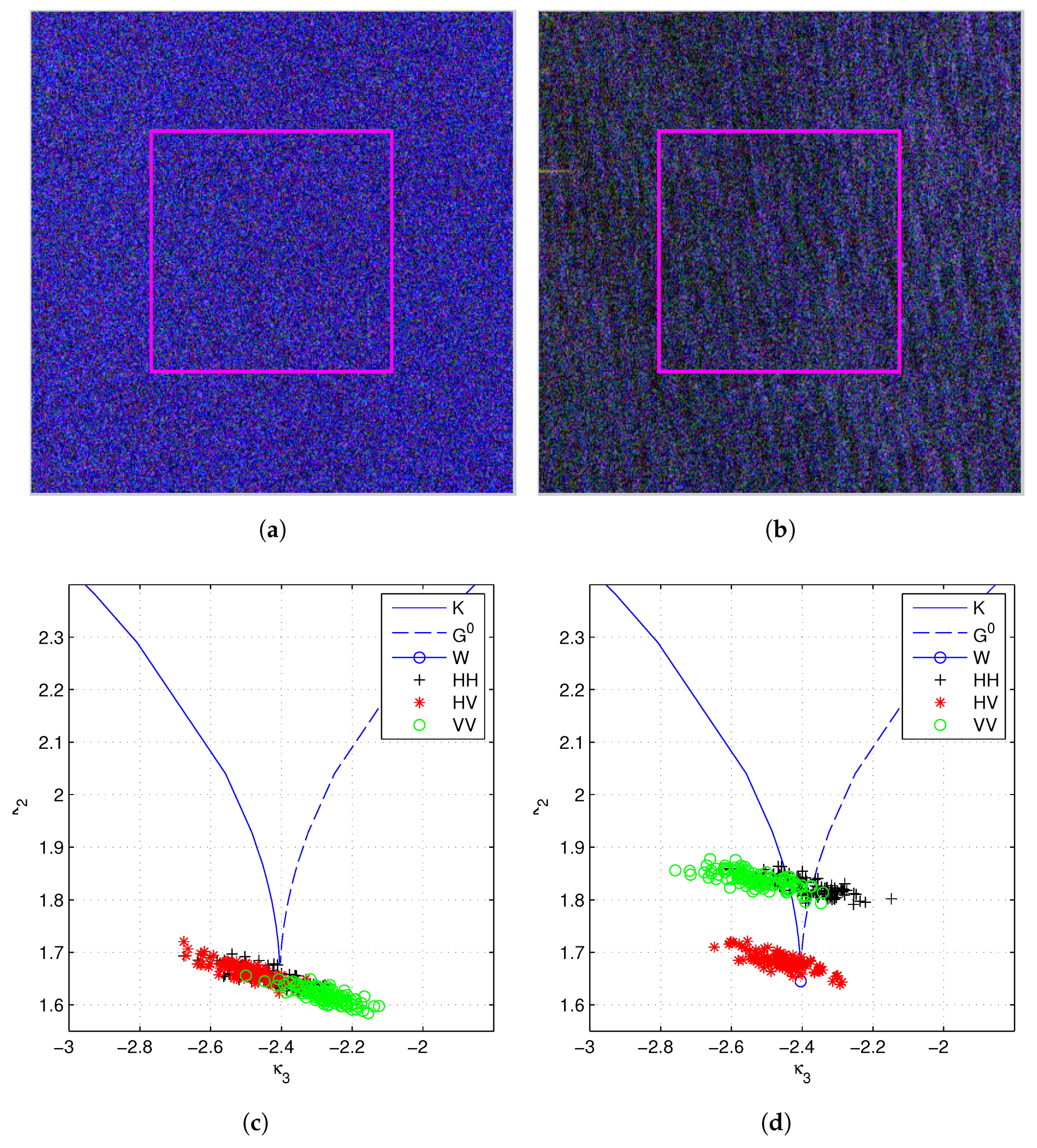
At last, statistical properties of the sea area at two different conditions are examined. One is with smooth surface, and the other with waves, as shown in Figure 7. Both data are acquired by RADARSAT-2 at C-band, and they have similar spatial resolutions. To study the textures of different polarimetric channels, the intensity of each channel is checked separately using the scalar log-cumulants [42,71]. The second order and the third order log-cumulants are employed as before. From Figure 7, we can see that in the first case, no texture is observed in all polarimetric channels. This can be also validated by the Pauli decomposition. When there exist sea waves, however, the log-cumulants are quite different. The HH channel and the VV channel have similar statistics, but different from those of the HV channel. In other words, multi-texture is observed in the test area. The result supposes that we can model the data using a dual-texture model in which the co-pol channels share a same texture distribution and the cross-pol channel with another one. The correlation between different textures needs to be further investigated to see if a partially correlated texture distribution is required.

Figure 7.
Scalar log-cumulants of different polarimetric channels (the HH, the HV and the VV channels) over sea areas. (a) Test region over smooth sea surface. (b) Test region over sea surface with waves. (c) Log-cumulants of the smooth sea surface. (d) Log-cumulants of the sea surface with waves.
7. Challenges
When the spatial resolution is not very high and the data is very homogeneous, the Gaussian distributions could provide a good representation of the data. As the spatial resolution increases, PolSAR data usually show non-Gaussian behaviour, e.g., exhibiting heavy tails. The texture models, which adopt additional random variables to model the spatial variation of the radar cross section, are found to be accurate for this kind of data. Texture models could model the non-Gaussian behavior observed in high resolution data, and yet keep a compact mathematical form. However, to model textures over complex scenes, sophisticated distributions are generally required. In addition, they are known to present problems in estimating parameters accurately. General distributions that cover a wide range of other distributions are suggested by many researchers. However, they usually have a complex form. Using several simple distributions from a certain family, Pearson family for example, could be a better idea. The distributions from a same family often have similar behaviors, but can be further distinguished by statistics like higher order log-cumulants [70].
In the product model as shown in (33) or (34), positive random variable following any distribution can be employed to model the texture. Additionally, PDFs of the scattering vector or the sample covariance matrix can be obtained subsequently after mathematical calculations. The PDFs, however, give no information about why the data following a specific distribution is obtained. Most of the texture models lack a physical explanation of the underlying scattering process. A possible way to solve this problem could be the random walk model, which treats the received signal as an addition of responses from all the scatterers in the same resolution cell [9,12,72]. The random walk model can be interpreted as a discrete analog of the SAR focusing process.
Texture information has been used in optical image processing for a long time. In SAR or PolSAR images, it is also found to be useful to distinguish different target types. For example, trees of different heights can be distinguished by texture information [73]. However, currently the most common way to make use of texture models is to design probability based algorithms (e.g., classification and segmentation) by replacing the Gaussian distribution or the Wishart distribution [4,5,6]. How to extract texture information and let PolSAR applications benefit from it is not involved. Apparently, combining polarimetric information and texture information could improve the performance of applications since more knowledge is introduced. Therefore, a further study in this aspect will be of great value.
Besides texture models, there are non-Gaussian models subdividing complicated distributions into components, each with a simple distribution. For example, the finite mixture model treats a distribution as a weighted sum of those of different target types. In addition, the copula based model divides a multivariate distribution into marginal distributions and a general dependence structure. In the finite mixture model, robust algorithms to estimate the mixing number and the mixing weights are in urgent need. For the copula based method, we have many options for the marginal distributions. However, for the dependence structure, not many experiments were implemented to show which copula is the best. Additionally, it is a big challenge to extend the bivariate copulas which are intensively investigated in the field of statistical analysis to multivariate ones to fit the PolSAR data.
The statistical properties of PolSAR data are characterized totally by the PDFs of the scattering vectors or the sample covariance matrices. However, it is difficult to use these PDFs directly because they are multivariate ones. Normally, the statistics of each polarimetric channel are studied separately, and the correlation between different polarimetric channels are neglected. Another way is to analyze the determinants of sample covariance matrices. The widely used matrix variate log-cumulant is an example. However, we need to filter the data (the multilook process) to obtain the sample covariance matrices, which could change the actual statistical properties of the data. To overcome these problems, the -norms of the scattering vectors can be employed, and they are found to be a useful tool for texture analysis of PolSAR data [73]. However, there are also limitations, e.g., the difference between models are not very large.
In summary, statistical modeling and texture analysis of PolSAR data covers a wide range of topics. To make a better understanding of texture and to make good use of it, there is still have a lot of work to do.
Acknowledgments
This work has been financed by: the Shenzhen Science & Technology Program with code JSGG20150512145714247, the Spanish Science, Research and Innovation Plan (Ministerio de Economía y Competitividad) with project code TIN2014-55413-C2-1-P, and the National Key Research Plan with code 2016YFC0500201-07. In addition, the authors would like to acknowledge ESA (European Space Agency) for the RADARSAT-2 data provided in the frame of the AgriSAR 2009 campaign, JAXA (Japan Aerospace Exploration Agency) for the ALOS-2 data provided in the framework of the 4th ALOS Research Announcement for ALOS-2, NASA (National Aeronautics and Space Administration) for the UAVSAR data, and Andreas Reigber from DLR for the F-SAR data.
Author Contributions
Xinping Deng designed and performed the experiments, analyzed the data, and wrote the paper; Carlos López-Martínez and Jinsong Chen provided valuable suggestions to write the paper, and revised the paper; Pengpeng Han prepared some of the data used in the experiments.
Conflicts of Interest
The authors declare no conflict of interest. The founding sponsors had no role in the design of the study; in the collection, analyses, or interpretation of data; in the writing of the manuscript, and in the decision to publish the results.
Abbreviations
The following abbreviations are used in this manuscript:
| BSA | Back Scattering Alignment |
| CDF | Cumulative Distribution Function |
| CLT | Central Limit Theorem |
| FSA | Forward Scattering Alignment |
| GIG | Generalized Inverse Gaussian |
| NIG | Normal Inverse Gaussian |
| NIM | Normalized Intensity Gaussian |
| Probability Density Function | |
| PolSAR | Polarimetric SAR |
| ROI | Region Of Interest |
| SAR | Synthetic Aperture Radar |
| SIRV | Spherically Invariant Random Vector |
Appendix A
Some integral identities used in this paper are listed out here.
- ([74] p. 368, Equation (3.471-9))is the modified Bessel function of the second kind of order v.
- ([74] p. 340, Equation (3.339))is the modified Bessel function of the first kind.
- ([74] p. 702, Equation (6.624-1))
- ([74] p. 347, Equation (3.382-2))
- ([74] p. 700, Equation (6.621-3))is the Gauss hypergeometric function.
- ([74] p. 917, Equation (8.432-3))
- ([74] p. 325, Equation (3.252-3))
- The gamma function is defined asLet where , we have the following equation after changing variables
- ([34] p. 505, Equation (13.2.5))U is the confluent hypergeometric function of the second kind, or KummerU function.
- ([74] p. 367, Equation (3.471-2))W is Whittaker W function.
- ([74] p. 368, Equation (3.471-5))M is the confluent hypergeometric function of the first kind, also known as the KummerM function.
References
- Goodman, J.W. Some fundamental properties of speckle. JOSA 1976, 66, 1145–1150. [Google Scholar] [CrossRef]
- Lee, J.S.; Grunes, M.R.; De Grandi, G. Polarimetric SAR speckle filtering and its implication for classification. IEEE Trans. Geosci. Remote Sens. 1999, 37, 2363–2373. [Google Scholar]
- Kersten, P.R.; Lee, J.S.; Ainsworth, T.L. Unsupervised classification of polarimetric synthetic aperture radar images using fuzzy clustering and EM clustering. IEEE Trans. Geosci. Remote Sens. 2005, 43, 519–527. [Google Scholar] [CrossRef]
- Doulgeris, A.P.; Anfinsen, S.N.; Eltoft, T. Classification with a non-Gaussian model for PolSAR data. IEEE Trans. Geosci. Remote Sens. 2008, 46, 2999–3009. [Google Scholar] [CrossRef]
- Bombrun, L.; Vasile, G.; Gay, M.; Totir, F. Hierarchical segmentation of polarimetric SAR images using heterogeneous clutter models. IEEE Trans. Geosci. Remote Sens. 2011, 49, 726–737. [Google Scholar] [CrossRef]
- Doulgeris, A.P.; Akbari, V.; Eltoft, T. Automatic PolSAR segmentation with the U-distribution and Markov random fields. In Proceedings of the 2012 EUSAR—9th European Conference on Synthetic Aperture Radar, Nuremberg, Germany, 23–26 April 2012; pp. 183–186. [Google Scholar]
- Lee, J.S.; Mitchell, R.G.; Kwok, R. Classification of multi-look polarimetric SAR imagery based on complex Wishart distribution. Int. J. Remote Sens. 1994, 15, 2299–2311. [Google Scholar] [CrossRef]
- Lee, J.S.; Grunes, M.; Ainsworth, T.; Du, L.J.; Schuler, D.; Cloude, S. Unsupervised classification using polarimetric decomposition and the complex Wishart classifier. IEEE Trans. Geosci. Remote Sens. 1999, 37, 2249–2258. [Google Scholar]
- Jakeman, E.; Pusey, P.N. A model for non-Rayleigh sea echo. IEEE Trans. Antennas Propag. 1976, 24, 806–814. [Google Scholar] [CrossRef]
- Jakeman, E.; Pusey, P. Significance of K distributions in scattering experiments. Phys. Rev. Lett. 1978, 40, 546–550. [Google Scholar] [CrossRef]
- Ward, K. Compound representation of high resolution sea clutter. Electron. Lett. 1981, 17, 561–563. [Google Scholar] [CrossRef]
- Yueh, S.H.; Kong, J.A.; Jao, J.K.; Shin, R.T.; Novak, L.M. K-distribution and polarimetric terrain radar clutter. J. Electromagn. Waves Appl. 1989, 3, 747–768. [Google Scholar] [CrossRef]
- Lee, J.S.; Schuler, D.L.; Lang, R.H.; Ranson, K.J. K-distribution for multi-look processed polarimetric SAR imagery. In Proceedings of the International Geoscience and Remote Sensing Symposium, Surface and Atmospheric Remote Sensing: Technologies, Data Analysis and Interpretation, Pasadena, CA, USA, 8–12 August 1994; Volume 4, pp. 2179–2181. [Google Scholar]
- Frery, A.C.; Muller, H.J.; Yanasse, C.C.F.; Sant’Anna, S.J.S. A model for extremely heterogeneous clutter. IEEE Trans. Geosci. Remote Sens. 1997, 35, 648–659. [Google Scholar] [CrossRef]
- Freitas, C.C.; Frery, A.C.; Correia, A.H. The polarimetric G distribution for SAR data analysis. Environmetrics 2005, 16, 13–31. [Google Scholar] [CrossRef]
- Bombrun, L.; Beaulieu, J.M. Fisher distribution for texture modeling of polarimetric SAR data. IEEE Geosci. Remote Sens. Lett. 2008, 5, 512–516. [Google Scholar] [CrossRef]
- Moser, G.; Zerubia, J.; Serpico, S.B. Dictionary-based stochastic expectation-maximization for SAR amplitude probability density function estimation. IEEE Trans. Geosci. Remote Sens. 2006, 44, 188–200. [Google Scholar] [CrossRef]
- Krylov, V.; Moser, G.; Serpico, S.B.; Zerubia, J. Modeling the Statistics of High Resolution SAR Images; Technical Report; Institut National de Recherche en Informatique et en Automatique, INRIA: Rocquencourt, France, 2008. [Google Scholar]
- Wang, Y.; Ainsworth, T.L.; Lee, J. On Characterizing High-Resolution SAR Imagery Using Kernel-Based Mixture Speckle Models. IEEE Geosci. Remote Sens. Lett. 2015, 12, 968–972. [Google Scholar] [CrossRef]
- Gao, G. Statistical modeling of SAR images: A survey. Sensors 2010, 10, 775–795. [Google Scholar] [CrossRef] [PubMed]
- Nelsen, R.B. An Introduction to Copulas; Springer Science & Business Media: New York, NY, USA, 2007. [Google Scholar]
- Mercier, G.; Bouchemakh, L.; Smara, Y. The use of multidimensional copulas to describe amplitude distribution of polarimetric SAR data. In Proceedings of the IEEE International Geoscience and Remote Sensing Symposium, Barcelona, Spain, 23–28 July 2007; pp. 2236–2239. [Google Scholar]
- Voisin, A.; Krylov, V.A.; Moser, G.; Serpico, S.B.; Zerubia, J. Supervised Classification of Multisensor and Multiresolution Remote Sensing Images With a Hierarchical Copula-Based Approach. IEEE Trans. Geosci. Remote Sens. 2014, 52, 3346–3358. [Google Scholar] [CrossRef]
- Lee, J.S.; Pottier, E. Polarimetric Radar Imaging: From Basics to Applications; CRC Press: Boca Raton, FL, USA, 2009. [Google Scholar]
- Cloude, S. Polarisation: Applications in Remote Sensing; Oxford University Press: Oxford, UK, 2009. [Google Scholar]
- Cloude, S.R.; Pottier, E. A review of target decomposition theorems in radar polarimetry. IEEE Trans. Geosci. Remote Sens. 1996, 34, 498–518. [Google Scholar] [CrossRef]
- Frost, V.S.; Stiles, J.A.; Shanmugan, K.S.; Holtzman, J.C. A Model for Radar Images and Its Application to Adaptive Digital Filtering of Multiplicative Noise. IEEE Trans. Pattern Anal. Mach. Intell. 1982, PAMI-4, 157–166. [Google Scholar] [CrossRef]
- Kong, J.; Yueh, S.; Lim, H.; Shin, R.; Van Zyl, J. Classification of earth terrain using polarimetric synthetic aperture radar images. Prog. Electromagn. Res. 1990, 3, 327–370. [Google Scholar]
- Sarabandi, K. Derivation of phase statistics from the Mueller matrix. Radio Sci. 1992, 27, 553. [Google Scholar] [CrossRef]
- Ulaby, F.; Sarabandi, K.; Nashashibi, A. Statistical properties of the Mueller matrix of distributed targets. In Proceedings of the IEE Proceedings F—Radar and Signal Processing, Barcelona, Spain, 6 August 1992; Volume 139, pp. 136–146. [Google Scholar]
- Goodman, N.R. Statistical analysis based on a certain multivariate complex Gaussian distribution (An Introduction). Ann. Math. Stat. 1963, 34, 152–177. [Google Scholar] [CrossRef]
- Lee, J.S.; Hoppel, K.W.; Mango, S.A.; Miller, A.R. Intensity and phase statistics of multilook polarimetric and interferometric SAR imagery. IEEE Trans. Geosci. Remote Sens. 1994, 32, 1017–1028. [Google Scholar]
- Tough, R.J.A.; Blacknell, D.; Quegan, S. A statistical description of polarimetric and interferometric synthetic aperture radar data. Proc. R. Soc. Lond. A Math. Phys. Sci. 1995, 449, 567–589. [Google Scholar] [CrossRef]
- Abramowitz, M.; Stegun, I.A. Handbook of Mathematical Functions: With Formulas, Graphs, and Mathematical Tables; Courier Corporation: North Chelmsford, MA, USA, 1964; Volume 55. [Google Scholar]
- Walck, C. Hand-Book on Statistical Distributions for Experimentalists; University of Stockholm: Stockholm, Sweden, 2007. [Google Scholar]
- López-Martínez, C.; Fabregas, X. Polarimetric SAR speckle noise model. IEEE Trans. Geosci. Remote Sens. 2003, 41, 2232–2242. [Google Scholar] [CrossRef]
- López-Martínez, C.; Pottier, E.; Cloude, S.R. Statistical assessment of eigenvector-based target decomposition theorems in radar polarimetry. IEEE Trans. Geosci. Remote Sens. 2005, 43, 2058–2074. [Google Scholar] [CrossRef]
- Alonso-González, A.; López-Martínez, C.; Salembier, P. Filtering and segmentation of polarimetric SAR data based on binary partition trees. IEEE Trans. Geosci. Remote Sens. 2012, 50, 593–605. [Google Scholar] [CrossRef]
- Anfinsen, S.N.; Eltoft, T.; Doulgeris, A.P. A relaxed Wishart model for polarimetric SAR data. In Proceedings of the Fourth International Workshop on Science and Applications of SAR Polarimetry and Polarimetric Interferometry PoIInSAR; European Space Agency: Noordwijk, The Netherlands, 2009; pp. 26–30. [Google Scholar]
- Kersten, P.R.; Anfinsen, S.N. A flexible and computationally efficient density model for the multilook polarimetric covariance matrix. In Proceedings of the 9th European Conference on Synthetic Aperture Radar, Nuremberg, Germany, 23–26 April 2012; pp. 760–763. [Google Scholar]
- Kersten, P.R.; Anfinsen, S.N.; Doulgeris, A.P. The Wishart-Kotz classifier for multilook polarimetric SAR data. In Proceedings of the IEEE International Geoscience and Remote Sensing Symposium, Munich, Germany, 22–27 July 2012; pp. 3146–3149. [Google Scholar]
- Anfinsen, S.N.; Eltoft, T. Application of the matrix-variate Mellin transform to analysis of polarimetric radar images. IEEE Trans. Geosci. Remote Sens. 2011, 49, 2281–2295. [Google Scholar] [CrossRef]
- Novak, L.M.; Burl, M.C. Optimal speckle reduction in polarimetric SAR imagery. IEEE Trans. Aerosp. Electron. Syst. 1990, 26, 293–305. [Google Scholar] [CrossRef]
- Sheen, D.R.; Johnston, L.P. Statistical and spatial properties of forest clutter measured with polarimetric synthetic aperture radar (SAR). IEEE Trans. Geosci. Remote Sens. 1992, 30, 578–588. [Google Scholar] [CrossRef]
- Gini, F.; Greco, M. Covariance matrix estimation for CFAR detection in correlated heavy tailed clutter. Signal Process. 2002, 82, 1847–1859. [Google Scholar] [CrossRef]
- Pascal, F.; Forster, P.; Ovarlez, J.; Larzabal, P. Performance analysis of covariance matrix estimates in impulsive noise. IEEE Trans. Signal Process. 2008, 56, 2206–2217. [Google Scholar] [CrossRef]
- Vasile, G.; Ovarlez, J.P.; Pascal, F.; Tison, C. Coherency matrix estimation of heterogeneous clutter in high-resolution polarimetric SAR images. IEEE Trans. Geosci. Remote Sens. 2010, 48, 1809–1826. [Google Scholar] [CrossRef]
- Bombrun, L.; Anfinsen, S.N.; Harant, O. A complete coverage of log-cumulant space in terms of distributions for Polarimetric SAR data. In Proceedings of the 5th International Workshop on Science and Applications of SAR Polarimetry and Polarimetric Interferometry (POLinSAR 2011), Friscati, Italy, 24–28 January 2011; pp. 1–8. [Google Scholar]
- Doulgeris, A.; Anfinsen, S.N.; Eltoft, T. Analysis of non-Gaussian POLSAR data. In Proceedings of the IEEE International Geoscience and Remote Sensing Symposiumm, Barcelona, Spain, 23–28 July 2007; pp. 160–163. [Google Scholar]
- Doulgeris, A.P.; Eltoft, T. Scale Mixture of Gaussian Modelling of Polarimetric SAR Data. EURASIP J. Adv. Signal Process. 2009, 2010, 874592. [Google Scholar]
- Koudou, A.E.; Ley, C. Characterizations of GIG laws: A survey. Probab. Surv. 2014, 11, 161–176. [Google Scholar] [CrossRef]
- Khan, S.; Guida, R. Application of Mellin-Kind Statistics to Polarimetric G Distribution for SAR Data. IEEE Trans. Geosci. Remote Sens. 2014, 52, 3513–3528. [Google Scholar] [CrossRef]
- Tison, C.; Nicolas, J.M.; Tupin, F.; Maître, H. A new statistical model for Markovian classification of urban areas in high-resolution SAR images. IEEE Trans. Geosci. Remote Sens. 2004, 42, 2046–2057. [Google Scholar] [CrossRef]
- Song, W.; Li, M.; Zhang, P.; Wu, Y.; Jia, L.; An, L. The WGΓ Distribution for Multilook Polarimetric SAR Data and Its Application. IEEE Geosci. Remote Sens. Lett. 2015, 12, 2056–2060. [Google Scholar] [CrossRef]
- Bian, Y.; Mercer, B. Multilook polarimetric SAR data probability density function estimation using a generalized form of multivariate K-distribution. Remote Sens. Lett. 2014, 5, 682–691. [Google Scholar] [CrossRef]
- De Grandi, G.; Lee, J.S.; Schuler, D.; Nezry, E. Texture and speckle statistics in polarimetric SAR synthesized images. IEEE Trans. Geosci. Remote Sens. 2003, 41, 2070–2088. [Google Scholar] [CrossRef]
- Eltoft, T.; Anfinsen, S.N.; Doulgeris, A.P. A multitexture model for multilook polarimetric radar data. In Proceedings of the IEEE International Geoscience and Remote Sensing Symposium, Vancouver, BC, Canada, 24–29 July 2011; pp. 1048–1051. [Google Scholar]
- Yu, Y. Textural-partially correlated polarimetric K-distribution. In Proceedings of the IEEE International Geoscience and Remote Sensing Symposium, Seattle, WA, USA, 6–10 July 1998; Volume 1, pp. 60–62. [Google Scholar]
- Eltoft, T.; Anfinsen, S.N.; Doulgeris, A.P. A multitexture model for multilook polarimetric synthetic aperture radar data. IEEE Trans. Geosci. Remote Sens. 2014, 52, 2910–2919. [Google Scholar] [CrossRef]
- Doulgeris, A.P.; Anfinsen, S.N.; Eltoft, T. Segmentation of polarimetric SAR data with a multi-texture product model. In Proceedings of the IEEE International Geoscience and Remote Sensing Symposium, Nuremberg, Germany, 22–27 July 2012; pp. 1437–1440. [Google Scholar]
- Lombardo, P.; Farina, A. Coherent radar detection against K-distributed clutter with partially correlated texture. Signal Process. 1996, 48, 1–15. [Google Scholar] [CrossRef]
- Khan, S.; Guida, R. The new dual-texutre G distribution for single-look PolSAR data. In Proceedings of the IEEE International Geoscience and Remote Sensing Symposium, Nuremberg, Germany, 22–27 July 2012; pp. 1469–1472. [Google Scholar]
- Anfinsen, S.N. Statistical Unmixing of SAR Images; Technical Report; Munin Open Research Archive, University of Tromsø—The Arctic University of Norway: Tromsø, Norway, 2016. [Google Scholar]
- Wang, Y.; Ainsworth, T.L.; Lee, J.S. Application of Mixture Regression for Improved Polarimetric SAR Speckle Filtering. IEEE Trans. Geosci. Remote Sens. 2017, 55, 453–467. [Google Scholar] [CrossRef]
- Frühwirth-Schnatter, S. Finite Mixture and Markov Switching Models; Springer: Berlin, Germany, 2006. [Google Scholar]
- McNeil, A.J.; Frey, R.; Embrechts, P. Quantitative Risk Management: Concepts, Techniques and Tools; Princeton University Press: Princeton, NJ, USA, 2005. [Google Scholar]
- Mercier, G.; Moser, G.; Serpico, S.B. Conditional copulas for change detection in heterogeneous remote sensing images. IEEE Trans. Geosci. Remote Sens. 2008, 46, 1428–1441. [Google Scholar] [CrossRef]
- Regniers, O.; Bombrun, L.; Guyon, D.; Samalens, J.C.; Germain, C. Wavelet-based texture features for the classification of age classes in a maritime pine forest. IEEE Geosci. Remote Sens. Lett. 2015, 12, 621–625. [Google Scholar] [CrossRef]
- Oliver, C. Fundamental properties of high-resolution sideways-looking radar. IEEE F-Commun. Radar Sig. 1982, 129, 385–402. [Google Scholar] [CrossRef]
- Deng, X.; López-Martínez, C. Higher Order Statistics for Texture Analysis and Physical Interpretation of Polarimetric SAR Data. IEEE Geosci. Remote Sens. Lett. 2016, 13, 912–916. [Google Scholar] [CrossRef]
- Nicolas, J.M. Introduction aux statistiques de deuxième espèce: Applications des logs-moments et des logs-cumulants à l’analyse des lois d’images radar. TS. Traitement du Signal 2002, 19, 139–167. [Google Scholar]
- Deng, X.; López-Martínez, C.; Varona, E.M. A Physical Analysis of Polarimetric SAR Data Statistical Models. IEEE Trans. Geosci. Remote Sens. 2016, 54, 3035–3048. [Google Scholar] [CrossRef]
- Deng, X.; López-Martínez, C. On the Use of the l2-Norm for Texture Analysis of Polarimetric SAR Data. IEEE Trans. Geosci. Remote Sens. 2016, 54, 6385–6398. [Google Scholar] [CrossRef]
- Jeffrey, A.; Zwillinger, D. Table of Integrals, Series, and Products, 7th ed.; Academic Press: Boston, MA, USA, 2007. [Google Scholar]

© 2017 by the authors. Licensee MDPI, Basel, Switzerland. This article is an open access article distributed under the terms and conditions of the Creative Commons Attribution (CC BY) license (http://creativecommons.org/licenses/by/4.0/).