
A Density-Based Clustering Method for Urban Scene Mobile Laser Scanning Data Segmentation


Abstract
:1. Introduction
2. Related Works
2.1. Euclidean Distance
2.2. Geometric Features
2.3. Other Features
3. Methods
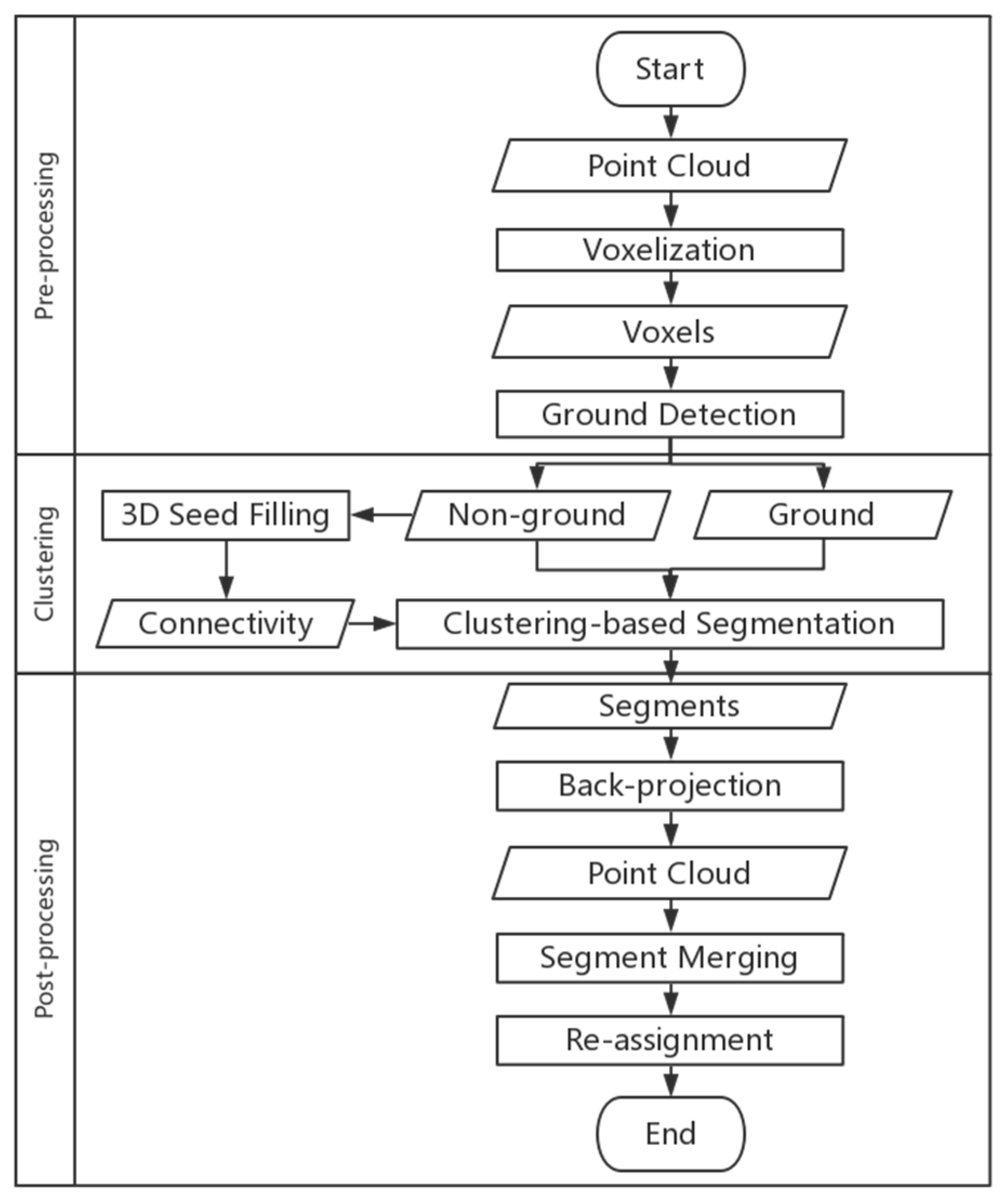
- Pre-processing: Original un-organized MLS data are cleaned and re-organized based on voxels; then, the whole scene is classified into ground and non-ground voxels.
- Clustering: A density-based clustering method is utilized to segment the non-ground voxels into discrete clusters.
- Post-processing: Voxels with cluster labels are back-projected points to merge clusters that belong to an individual street object accurately, and noise points generated in the clustering stage are re-assigned to the clusters.
3.1. Pre-Processing
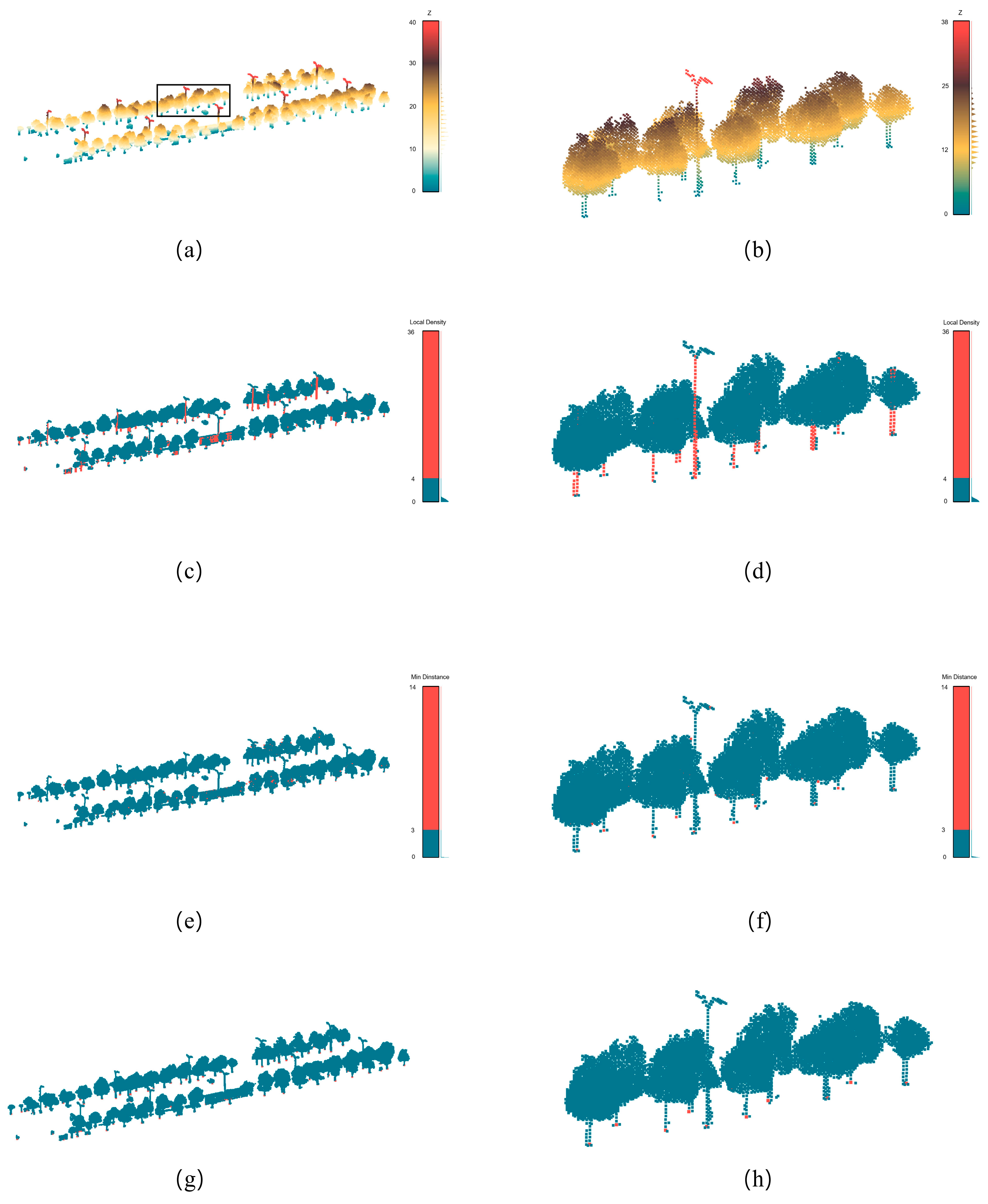
3.1.1. Voxelization
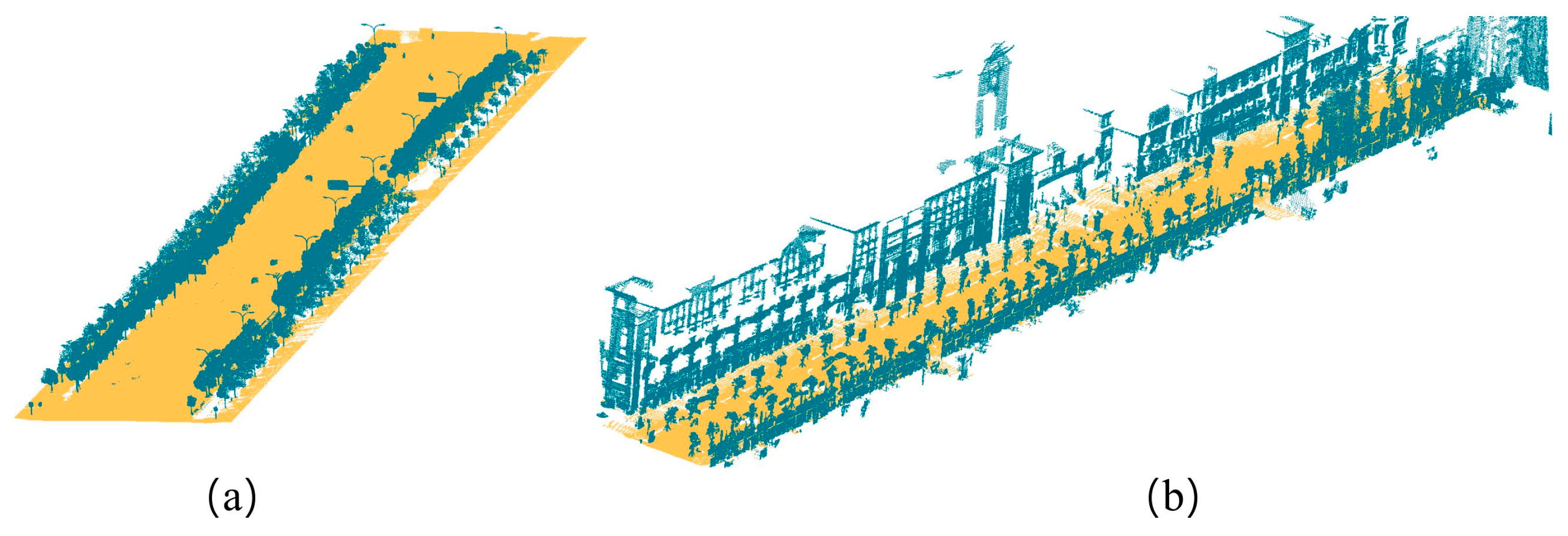
3.1.2. Ground Detection
3.2. Clustering
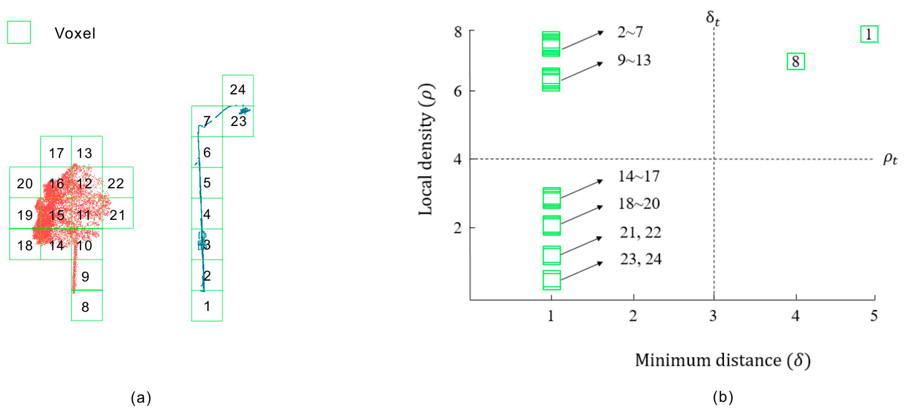
3.2.1. Generation of Cluster Centers
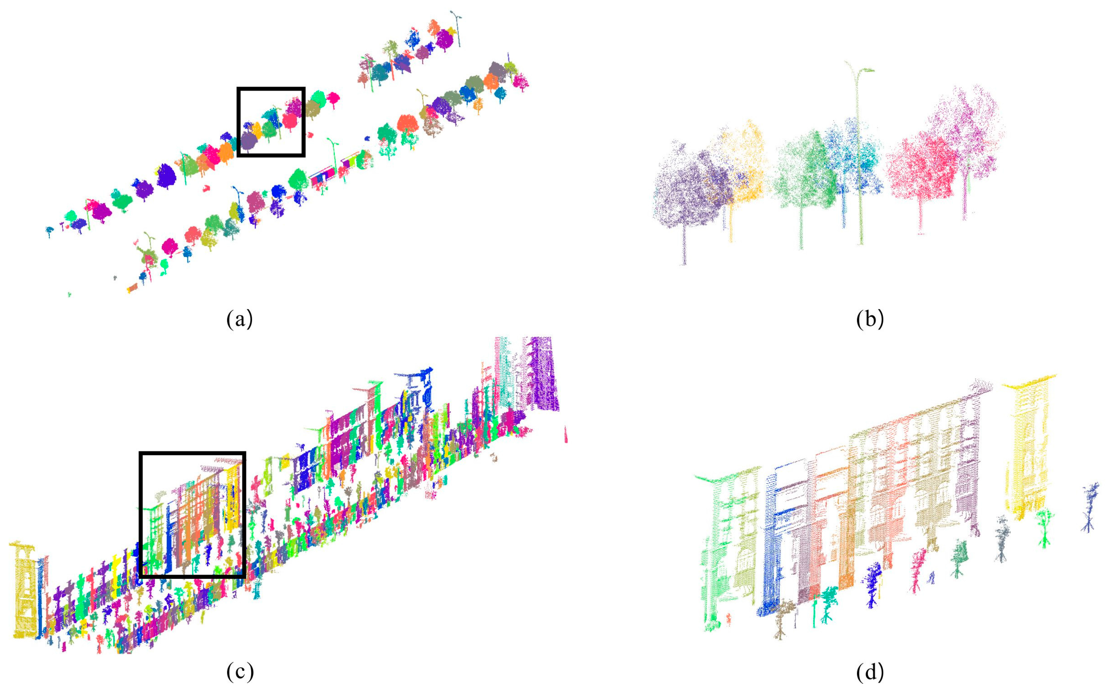
3.2.2. Clustering
| Algorithm 1: Clustering |
| Input: |
| : voxel set for clustering |
| Parameters: |
| N: total amount of voxel |
| : radius for searching closest neighbors |
| Start: |
| (1) Calculate R = based on Equation (3). |
| (2) Sort R by descending order SR = . |
| (3) Calculate D = from Equation (6). |
| (4) Calculate CN = from Equation (9). |
| (5) Initialize the label of each voxel from Equation (8). |
| (6) for each voxel in SR repeat: |
| (7) if |
| (8) |
| End |
| Output: |
| C: cluster labels of |
3.3. Post-Processing
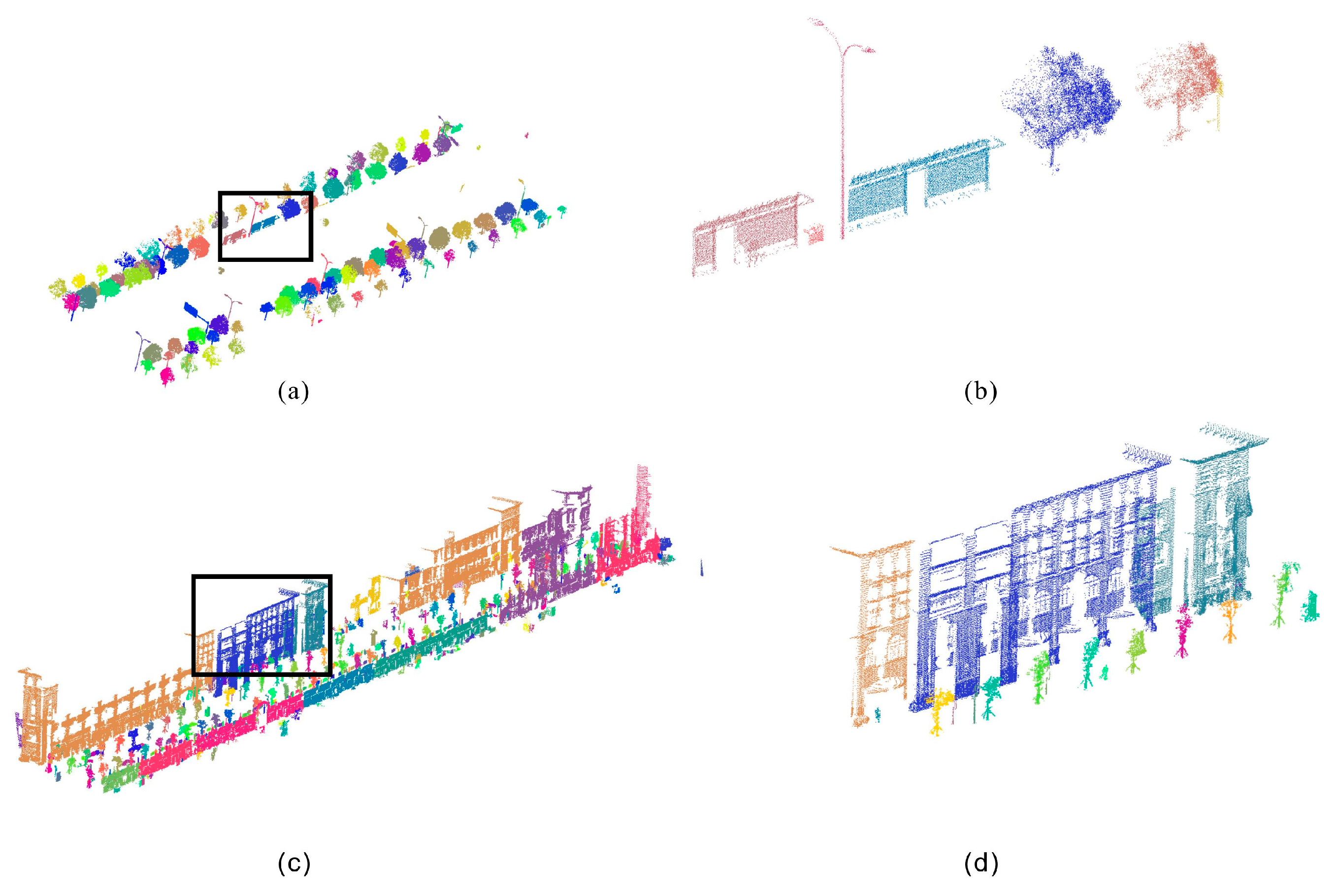
3.3.1. Merging of Clusters
3.3.2. Re-Assignment
4. Experiments
4.1. Voxelization and Ground Detection Results
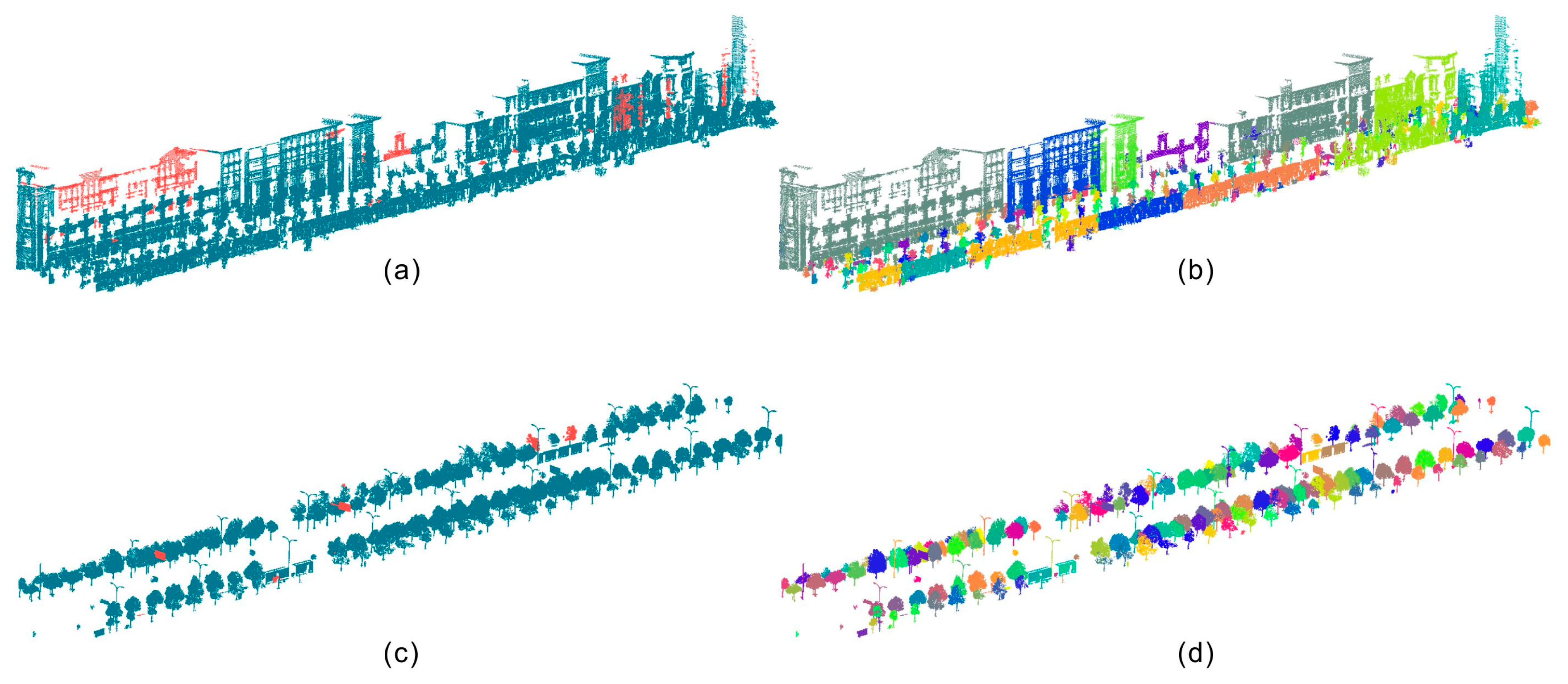
4.2. Clustering Results
4.3. Merging and Re-Assignment Results
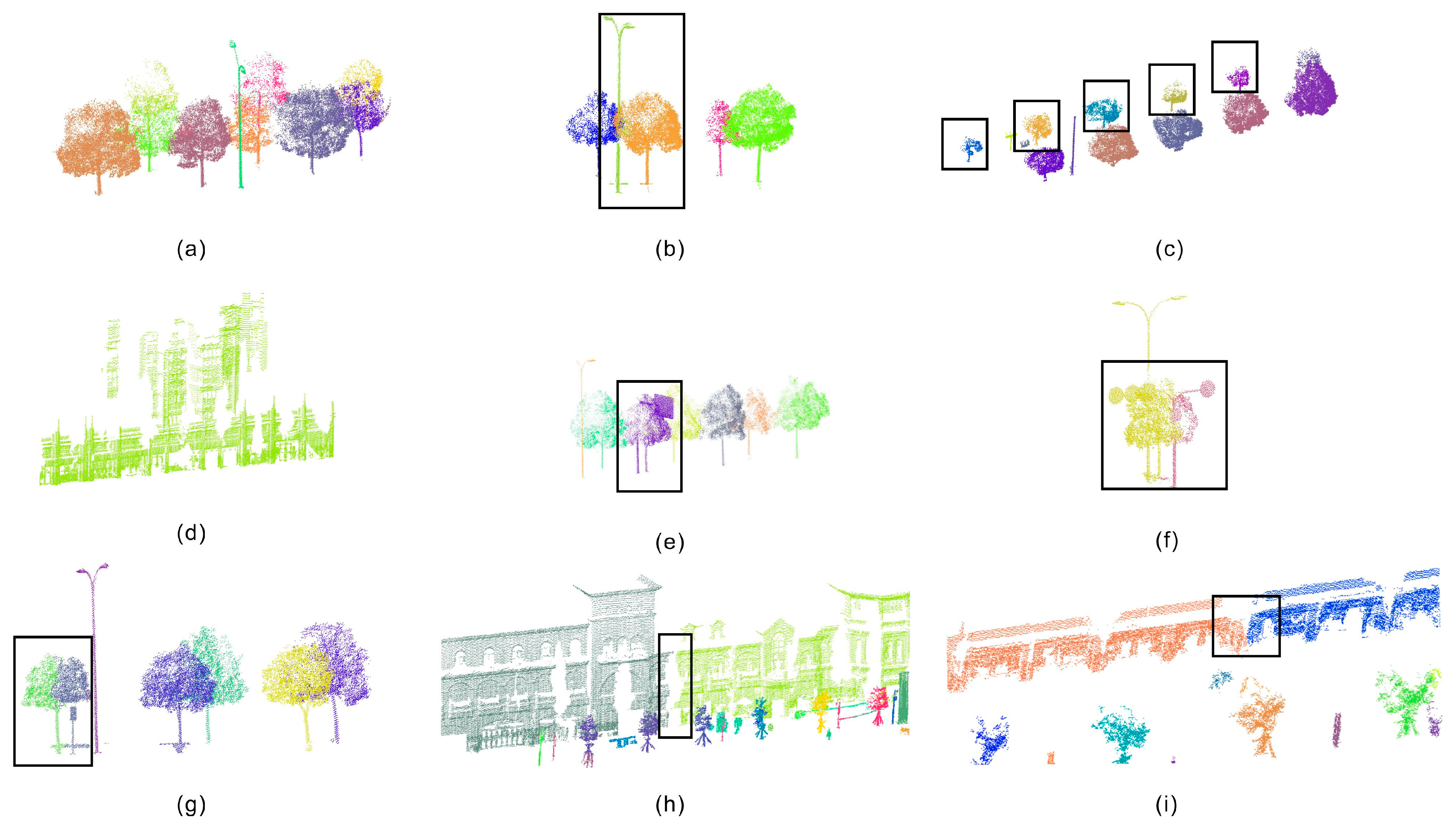
4.4. Performance Analysis of the Final Results
5. Conclusions
Acknowledgments
Author Contributions
Conflicts of Interest
References
- Sampath, A.; Shan, J. Segmentation and reconstruction of polyhedral building roofs from aerial LIDAR point clouds. IEEE Trans. Geosci. Remote Sens. 2010, 48, 1554–1567. [Google Scholar] [CrossRef]
- Rodríguez-Cuenca, B.; García-Cortés, S.; Ordóñez, C.; Alonso, M.C. An approach to detect and delineate street curbs from MLS 3D point cloud data. Autom. Constr. 2015, 51, 103–112. [Google Scholar] [CrossRef]
- Pu, S.; Rutzinger, M.; Vosselman, G.; Oude Elberink, S. Recognizing basic structures from mobile laser scanning data for road inventory studies. ISPRS J. Photogramm. Remote Sens. 2011, 66, S28–S39. [Google Scholar] [CrossRef]
- Brenner, C. Global localization of vehicles using local pole patterns. In Pattern Recognition; Springer: Berlin/Heidelberg, Germany, 2009; pp. 61–70. [Google Scholar]
- Zhang, C.; Zhou, Y.; Qiu, F. Individual tree segmentation from lidar point clouds for urban forest inventory. Remote Sens. 2015, 7, 7892–7913. [Google Scholar] [CrossRef]
- Yang, B.; Fang, L.; Li, J. Semi-automated extraction and delineation of 3D roads of street scene from mobile laser scanning point clouds. ISPRS J. Photogramm. Remote Sens. 2013, 79, 80–93. [Google Scholar] [CrossRef]
- Chen, D.; He, X. Fast automatic three-dimensional road model reconstruction based on mobile laser scanning system. Opt. Int. J. Light Electron Opt. 2015, 126, 725–730. [Google Scholar] [CrossRef]
- Yang, B.; Fang, L.; Li, Q.; Li, J. Automated extraction of road markings from mobile LIDAR point clouds. Photogramm. Eng. Remote Sens. 2012, 78, 331–338. [Google Scholar] [CrossRef]
- Li, L.; Zhang, D.; Ying, S.; Li, Y. Recognition and reconstruction of zebra crossings on roads from mobile laser scanning data. ISPRS Int. J. Geo-Inf. 2016, 5, 125. [Google Scholar] [CrossRef]
- Guan, H.; Li, J.; Yu, Y.; Wang, C.; Chapman, M.; Yang, B. Using mobile laser scanning data for automated extraction of road markings. ISPRS J. Photogramm. Remote Sens. 2014, 87, 93–107. [Google Scholar] [CrossRef]
- Pu, S.; Vosselman, G. Knowledge based reconstruction of building models from terrestrial laser scanning data. ISPRS J. Photogramm. Remote Sens. 2009, 64, 575–584. [Google Scholar] [CrossRef]
- Jochem, A.; Höfle, B.; Rutzinger, M. Extraction of vertical walls from mobile laser scanning data for solar potential assessment. Remote Sens. 2011, 3, 650–667. [Google Scholar] [CrossRef]
- Vo, A.-V.; Truong-Hong, L.; Laefer, D.F.; Bertolotto, M. Octree-based region growing for point cloud segmentation. ISPRS J. Photogramm. Remote Sens. 2015, 104, 88–100. [Google Scholar] [CrossRef]
- Li, L.; Li, Y.; Li, D. A method based on an adaptive radius cylinder model for detecting pole-like objects in mobile laser scanning data. Remote Sens. Lett. 2016, 7, 249–258. [Google Scholar] [CrossRef]
- Cabo, C.; Ordóñez, C.; García-Cortés, S.; Martínez, J. An algorithm for automatic detection of pole-like street furniture objects from mobile laser scanner point clouds. ISPRS J. Photogramm. Remote Sens. 2014, 87, 47–56. [Google Scholar] [CrossRef]
- Li, L.; Li, D.; Zhu, H.; Li, Y. A dual growing method for the automatic extraction of individual trees from mobile laser scanning data. ISPRS J. Photogramm. Remote Sens. 2016, 120, 37–52. [Google Scholar] [CrossRef]
- Wu, B.; Yu, B.; Yue, W.; Shu, S.; Tan, W.; Hu, C.; Huang, Y.; Wu, J.; Liu, H. A voxel-based method for automated identification and morphological parameters estimation of individual street trees from mobile laser scanning data. Remote Sens. 2013, 5, 584–611. [Google Scholar] [CrossRef]
- Rutzinger, M.; Pratihast, A.; Oude Elberink, S.; Vosselman, G. Detection and modelling of 3D trees from mobile laser scanning data. Int. Arch. Photogramm. Remote Sens. Spat. Inf. Sci. 2010, 38, 520–525. [Google Scholar]
- Zhou, Y.; Yu, Y.; Lu, G.; Du, S. Super-segments based classification of 3d urban street scenes. Int. J. Adv. Robot. Syst. 2012. [Google Scholar] [CrossRef]
- Yang, B.; Zhen, D. A shape based segmentation method for mobile laser scanning point clouds. ISPRS J. Photogramm. Remote Sens. 2013, 81, 19. [Google Scholar] [CrossRef]
- Yang, B.; Dong, Z.; Zhao, G.; Dai, W. Hierarchical extraction of urban objects from mobile laser scanning data. ISPRS J. Photogramm. Remote Sens. 2015, 99, 45–57. [Google Scholar] [CrossRef]
- Vosselman, G. Point cloud segmentation for urban scene classification. ISPRS Int. Arch. Photogramm. Remote Sens. Spat. Inf. Sci. 2013, 1, 257–262. [Google Scholar] [CrossRef]
- Aijazi, A.; Checchin, P.; Trassoudaine, L. Segmentation based classification of 3D urban point clouds: A super-voxel based approach with evaluation. Remote Sens. 2013, 5, 1624–1650. [Google Scholar] [CrossRef]
- Barnea, S.; Filin, S. Segmentation of terrestrial laser scanning data using geometry and image information. ISPRS J. Photogramm. Remote Sens. 2013, 76, 33–48. [Google Scholar] [CrossRef]
- Filin, S.; Pfeifer, N. Segmentation of airborne laser scanning data using a slope adaptive neighborhood. ISPRS J. Photogramm. Remote Sens. 2006, 60, 71–80. [Google Scholar] [CrossRef]
- Oude Elberink, S.; Kemboi, B. User-assisted object detection by segment based similarity measures in mobile laser scanner data. ISPRS Int. Arch. Photogramm. Remote Sens. Spat. Inf. Sci. 2014. [Google Scholar] [CrossRef]
- Zhou, Y.; Wang, D.; Xie, X.; Ren, Y.; Li, G.; Deng, Y.; Wang, Z. A fast and accurate segmentation method for ordered lidar point cloud of large-scale scenes. IEEE Geosci. Remote Sens. Lett. 2014, 11, 1981–1985. [Google Scholar] [CrossRef]
- El-Halawanya, S.I.; Lichtia, D.D. Detecting road poles from mobile terrestrial laser scanning data. GISci. Remote Sens. 2013, 50, 704–722. [Google Scholar]
- Golovinskiy, A.; Kim, V.G.; Funkhouser, T. Shape-based recognition of 3d point clouds in urban environments. In Proceedings of the 2009 IEEE 12th International Conference on Computer Vision, Kyoto, Japan, 27 September–4 October 2009. [Google Scholar]
- Vosselman, G.; Gorte, B.; Sithole, G.; Rabbani, T. Recognising structure in laser scanner point clouds. Int. Arch. Photogramm. Remote Sens. Spat. Inf. Sci. 2004. [Google Scholar] [CrossRef]
- Rabbani, T.; van den Heuvel, F.; Vosselmann, G. Segmentation of point clouds using smoothness constraint. Int. Arch. Photogramm. Remote Sens. Spat. Inf. Sci. 2006, 36, 248–253. [Google Scholar]
- Rodríguez-Cuenca, B.; García-Cortés, S.; Ordóñez, C.; Alonso, M. Automatic detection and classification of pole-like objects in urban point cloud data using an anomaly detection algorithm. Remote Sens. 2015, 7, 12680–12703. [Google Scholar] [CrossRef]
- Demantké, J.; Mallet, C.; David, N.; Vallet, B. Dimensionality based scale selection in 3d lidar point clouds. Int. Arch. Photogramm. Remote Sens. Spat. Inf. Sci. 2011. [Google Scholar] [CrossRef]
- Toth, C.; Paska, E.; Brzezinska, D. Using road pavement markings as ground control for lidar data. Int. Arch. Photogramm. Remote Sens. Spat. Inf. Sci. 2008, 37, 189–195. [Google Scholar]
- Riveiro, B.; González-Jorge, H.; Martínez-Sánchez, J.; Díaz-Vilariño, L.; Arias, P. Automatic detection of zebra crossings from mobile lidar data. Opt. Laser Technol. 2015, 70, 63–70. [Google Scholar] [CrossRef]
- Kumar, P.; McElhinney, C.P.; Lewis, P.; McCarthy, T. Automated road markings extraction from mobile laser scanning data. Int. J. Appl. Earth Obs. Geoinf. 2014, 32, 125–137. [Google Scholar] [CrossRef]
- Chen, X.; Kohlmeyer, B.; Stroila, M.; Alwar, N.; Wang, R.; Bach, J. Next generation map making: Geo-referenced ground-level lidar point clouds for automatic retro-reflective road feature extraction. In Proceedings of the 17th ACM SIGSPATIAL International Conference on Advances in Geographic Information Systems, Seattle, WA, USA, 4–6 November 2009; pp. 488–491. [Google Scholar]
- Tighe, J.; Niethammer, M.; Lazebnik, S. Scene parsing with object instances and occlusion ordering. In Proceedings of the 2014 IEEE Conference on Computer Vision and Pattern Recognition, Columbus, OH, USA, 23–28 June 2014; pp. 3748–3755. [Google Scholar]
- Golparvar-Fard, M.; Balali, V.; Garza, J.M.D.L. Segmentation and recognition of highway assets using image-based 3d point clouds and semantic texton forests. J. Comput. Civ. Eng. 2012, 29. [Google Scholar] [CrossRef]
- Balali, V.; Golparvar-Fard, M. Segmentation and recognition of roadway assets from car-mounted camera video streams using a scalable non-parametric image parsing method. Autom. Constr. 2015, 49, 27–39. [Google Scholar] [CrossRef]
- Balali, V.; Golparvarfard, M. Recognition and 3d localization of traffic signs via image-based point cloud models. In Proceedings of the 2015 International Workshop on Computing in Civil Engineering, Austin, TX, USA, 21–23 June 2015. [Google Scholar]
- Guan, H.; Li, J.; Yu, Y.; Chapman, M.; Wang, H.; Wang, C.; Zhai, R. Iterative tensor voting for pavement crack extraction using mobile laser scanning data. IEEE Trans. Geosci. Remote Sens. 2015, 53, 1527–1537. [Google Scholar] [CrossRef]
- Rodriguez, A.; Laio, A. Clustering by fast search and find of density peaks. Science 2014, 344, 1492–1496. [Google Scholar] [CrossRef] [PubMed]
- Serna, A.; Marcotegui, B. Detection, segmentation and classification of 3d urban objects using mathematical morphology and supervised learning. ISPRS J. Photogramm. Remote Sens. 2014, 93, 243–255. [Google Scholar] [CrossRef]


| Test Sites | Length (m) | Average Width (m) | Points (million) | Density (Points/m2) |
|---|---|---|---|---|
| Test site 1 (TS-1) | 303 | 60 | 6.8 | 374 |
| Test site 2(TS-2) | 285 | 30 | 2 | 234 |
| Parameters | Values | Number of Voxels |
|---|---|---|
| Local density threshold | 1.2 m | 4 |
| Minimum distance threshold | 0.9 m | 3 |
| Ground distance threshold ( | 1.5 m | 5 |
| Neighbor search radius () | 3.9 m | 13 |
| Sites | Trees | Pole-like objects | Cars | Buildings | Overall accuracy (OA) | |
|---|---|---|---|---|---|---|
| TS-1 | Under-segmentation rate(USR) | 2/140 | 3/28 | 0/9 | 0/0 | 98.3% |
| Over-segmentation rate (OSR) | 1/140 | 0/28 | 0/9 | 0/0 | ||
| TS-2 | Under-segmentation rate(USR) | 2/66 | 2/51 | 0/8 | 0/7 | 97% |
| Over-segmentation rate(OSR) | 1/66 | 0/51 | 0/8 | 3/7 |
© 2017 by the authors. Licensee MDPI, Basel, Switzerland. This article is an open access article distributed under the terms and conditions of the Creative Commons Attribution (CC BY) license (http://creativecommons.org/licenses/by/4.0/).
Share and Cite
Li, Y.; Li, L.; Li, D.; Yang, F.; Liu, Y. A Density-Based Clustering Method for Urban Scene Mobile Laser Scanning Data Segmentation. Remote Sens. 2017, 9, 331. https://doi.org/10.3390/rs9040331
Li Y, Li L, Li D, Yang F, Liu Y. A Density-Based Clustering Method for Urban Scene Mobile Laser Scanning Data Segmentation. Remote Sensing. 2017; 9(4):331. https://doi.org/10.3390/rs9040331
Chicago/Turabian StyleLi, You, Lin Li, Dalin Li, Fan Yang, and Yu Liu. 2017. "A Density-Based Clustering Method for Urban Scene Mobile Laser Scanning Data Segmentation" Remote Sensing 9, no. 4: 331. https://doi.org/10.3390/rs9040331
APA StyleLi, Y., Li, L., Li, D., Yang, F., & Liu, Y. (2017). A Density-Based Clustering Method for Urban Scene Mobile Laser Scanning Data Segmentation. Remote Sensing, 9(4), 331. https://doi.org/10.3390/rs9040331