Texture-Guided Multisensor Superresolution for Remotely Sensed Images

Abstract

This paper presents a novel technique, namely texture-guided multisensor superresolution (TGMS), for fusing a pair of multisensor multiresolution images to enhance the spatial resolution of a lower-resolution data source. TGMS is based on multiresolution analysis, taking object structures and image textures in the higher-resolution image into consideration. TGMS is designed to be robust against misregistration and the resolution ratio and applicable to a wide variety of multisensor superresolution problems in remote sensing. The proposed methodology is applied to six different types of multisensor superresolution, which fuse the following image pairs: multispectral and panchromatic images, hyperspectral and panchromatic images, hyperspectral and multispectral images, optical and synthetic aperture radar images, thermal-hyperspectral and RGB images, and digital elevation model and multispectral images. The experimental results demonstrate the effectiveness and high general versatility of TGMS.

1. Introduction

Multisensor superresolution is a technique for enhancing the spatial resolution of a low-resolution (LR) image by fusing it with an auxiliary high-resolution (HR) image obtained by a different imaging sensor. The spatial resolution of remote sensing instruments is often designed at a moderate or large scale due to the trade-off between sensor specifications, such as spatial resolution, spectral resolution, swath width, and signal-to-noise ratio. Therefore, there is always demand for enhancing the spatial resolution of remotely sensed images. Multisensor superresolution has been widely used in the remote sensing community to address the issue of spatial resolution by using complementary data sources.

Pan-sharpening is the most common multisensor superresolution technique, where an LR multispectral (MS) image is sharpened by fusing it with an HR panchromatic (PAN) image. Nowadays, many spaceborne MS sensors are mounted together with PAN sensors, and pan-sharpened products are distributed as default. Many pan-sharpening algorithms have been developed over the last three decades [1,2,3]. Component substitution (CS) methods [4,5,6] and multiresolution analysis (MRA) methods [7,8] are representative techniques and widely used as benchmark methods. Geostatistical methods based on kriging have been successfully applied to pan-sharpening [9] and multiband image fusion [10,11,12]. Sparse representation-based methods have recently demonstrated their promising performance [13,14,15].

With the advance of anticipated upcoming spaceborne hyperspectral (HS) missions [16,17,18,19,20,21,22], the resolution enhancement of spaceborne HS imagery has received considerable attention recently [23,24,25,26]. HS pan-sharpening [25] is naturally one option for enhancing the resolution of HS data using PAN imagery possibly obtained from the same platform (e.g., PRISMA [18] and SHALOM [22]). HS and MS data fusion is one of the most actively addressed tasks for creating HR-HS data with high spectral quality [26]. Subspace-based methods have been actively developed for HS-MS fusion [27,28,29], and pan-sharpening methods have also been adapted to the HS-MS fusion problem [30,31].

Enormous efforts have also been made to design multisensor superresolution techniques for multimodal data, where two input images are acquired by measuring entirely different characteristics of the surface via heterogeneous imaging systems. For instance, the fusion of visible near-infrared and thermal images to create an HR thermal image has been studied using Landsat data sets as early as 1990 [32]. The resolution enhancement of a digital elevation model (DEM) using an HR image was discussed for urban analysis in [33,34]. In [35], with the advent of HR synthetic aperture radar (SAR), an attempt has been made to increase the spatial resolution of optical (MS and PAN) images using SAR images as supporting materials.

Most of the multisensor superresolution methods in the literature have been designed for specific fusion problems. To develop a general framework for multisensor superresolution, there are challenges involved in dealing with sensor types and combinations and spatial characteristics, including the resolution ratio and misregistration. To the best of the author’s knowledge, a versatile multisensor superresolution methodology has not been fully developed.

This paper presents a novel technique, namely texture-guided multisensor superresolution (TGMS), for a wide variety of multisensor superresolution tasks. TGMS is based on MRA, considering object structures and texture information. Multiscale gradient descent is applied to MRA and improve superresolution performance at object boundaries by considering object structures at a high level (low resolution). Texture-guided filtering is proposed as a new intensity modulation technique where texture information is exploited to improve robustness against misregistration. The main contributions of this work are summarized as follows.

• Versatile methodology: This paper proposes a versatile methodology for multisensor superresolution in remote sensing.
• Comprehensive evaluation: This paper demonstrates six different types of multisensor superresolution, which fuse the following image pairs: MS-PAN images (MS pan-sharpening), HS-PAN images (HS pan-sharpening), HS-MS images, optical-SAR images, long-wavelength infrared (LWIR) HS and RGB images, and DEM-MS images. The performance of TGMS is evaluated both quantitatively and qualitatively.

The remainder of the paper is organized as follows. Section 2 describes the proposed technique. Section 3 is devoted to evaluation methodology. Section 4 and Section 5 present experimental results on optical data fusion and multimodal data fusion, respectively. Section 6 discusses findings and limitations of this work. Section 7 wraps up the paper by providing the main concluding remarks.

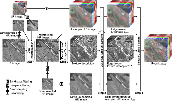
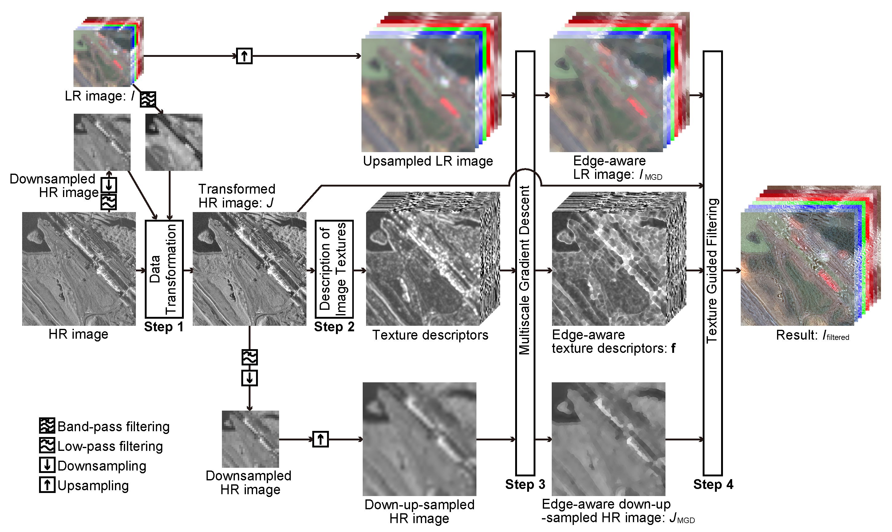
2. Texture-Guided Multisensor Superresolution

Figure 1 illustrates the flowchart describing the fusion process of the proposed technique (TGMS), using optical-SAR fusion as an example. TGMS is mainly composed of the following four steps: (1) data transformation of the HR image; (2) description of image textures in the HR image; (3) multiscale gradient descent; (4) texture-guided filtering. TGMS can be regarded as an MRA-based technique taking object structures and HR texture information into consideration. The key idea is to add spatial details to the LR image on the basis of local objects derived from the texture information of the HR image. The assumption behind this idea is that pixels recognized as belonging to the same object according to texture descriptors in the HR image have similar pixel features (e.g., spectral features in the case that spectral data is used for the LR image) in the output image. The four steps are detailed in the following subsections.

2.1. Data Transformation

The first step of the proposed methodology is data transformation of the HR image to make its pixel values correlated and consistent with the LR image. This procedure is important because proportionality of pixel values between the transformed HR and LR images is assumed on each object in the final step (i.e., texture-guided filtering). Depending on different types of data fusion regarding numbers of bands in the input LR-HR images, the first step adopts two kinds of data transformation for the HR image—namely, histogram matching and linear regression (see

Table 1. Data transformation of HR images for six types of data fusion under investigation.

Type of Fusion	Num. of Bands		Data Transform of HR Data
	LR	HR
MS-PAN	Multiple	One	Histogram matching
HS-PAN	Multiple	One	Histogram matching
Optical-SAR	Multiple	One	Histogram matching
HS-MS	Multiple	Multiple	Linear regression
DEM-MS	One	Multiple	Local linear regression
LWIR-HS-RGB	Multiple	Multiple	Linear regression

).

When the number of bands in the HR image is equal to one and that of the LR image is more than one, we first create a synthetic (or band-pass filtered) LR image as a linear combination of the LR bands using coefficients obtained by performing nonnegative least squares regression using the LR bands as explanatory variables and the downsampled HR image as a response variable. Next, histogram matching is performed on the HR image with the synthetic LR image being the target. If the regression error is very small in the first step (e.g., the coefficient of determination is larger than 0.9), the data transformation procedure is not required for the HR image (e.g., pan-sharpening experiments in this work).

When the HR image includes multiple bands (e.g., HS-MS fusion and LWIR-HS-RGB fusion), linear regression is used for data transformation. If the LR-HR images are of the same type, linear regression is performed for each LR band at the low resolution. By transforming the HR image using the obtained weighting coefficient, an HR synthetic image corresponding to each band of the LR image is obtained. If the input images are completely different types (or multimodal), a more particular technique is required depending on their data types. For example, in the case of DEM-MS fusion, linear regression is performed locally using segmentation (e.g., k-means) of the HR image. For LWIR-HS-RGB fusion, linear regression is performed only once, with the mean image of the LWIR-HS bands being the target. The transformed HR image is used to enhance the spatial resolution of all bands of the LWIR-HS image so that the fused image includes only natural spectral signatures (linear combinations of the measured spectra) but not artifacts.

2.2. Texture Descriptors

Description of texture information in the HR image is a key process in the proposed methodology to recognize local objects (or structures) based on similarity of texture descriptors. TGMS uses statistical texture descriptors presented in [36] based on region covariance [37,38] because of its efficient and compact way of encoding local structure and texture information via first- and second-order statistics in local regions.

Region covariance captures the underlying spatial characteristic by computing second-order statistics on d-dimensional image features, including the intensity and the gradient. Let $\mathbf{z}\left(\mathbf{p}\right)$ denote a d-dimensional feature vector at a pixel $\mathbf{p}=(x,y)$. The region covariance ${\mathbf{C}}_r\in {\mathbb{R}}^{d\times d}$ is defined by

$${\mathbf{C}}_r\left(\mathbf{p}\right)=\frac{1}{W}\sum _{{\mathbf{p}}_i\in {\Omega }_r}(\mathbf{z}\left({\mathbf{p}}_i\right)-{\overline{\mathbf{z}}}_r){(\mathbf{z}\left({\mathbf{p}}_i\right)-{\overline{\mathbf{z}}}_r)}^T{w}_r(\mathbf{p},{\mathbf{p}}_i),$$

(1)

where ${\Omega }_r$ is the $(2r+1)\times (2r+1)$ window centered at $\mathbf{p}$ and ${\overline{\mathbf{z}}}_r$ is the mean feature vector in the window. $w_r$ is a Gaussian weighting function defined by $w_r(\mathbf{p},{\mathbf{p}}_i)=exp\left(\frac{-9\parallel \mathbf{p}-{\mathbf{p}}_i{\parallel }_2^2}{2r^2}\right)$ to make local spatial features smoothly defined in the spatial domain and W is its normalization coefficient defined by $W={\sum }_{{\mathbf{p}}_i\in {\Omega }_r}{w}_r(\mathbf{p},{\mathbf{p}}_i)$. The scale r is set to be one half of the ratio between ground sampling distances (GSDs) of the input LR-HR images. For d-dimensional features of a grayscale image I, we use six features ($d=6$) composed of the original pixel value, and the first and second derivatives as

$$\mathbf{z}\left(\mathbf{p}\right)={\left[I(x,y)\left|\frac{\partial I}{\partial x}\right|\left|\frac{\partial I}{\partial y}\right|\left|\frac{{\partial }^{2}I}{\partial x^2}\right|\left|\frac{{\partial }^{2}I}{\partial y^2}\right|\left|\frac{{\partial }^{2}I}{\partial x\partial y}\right|\right]}^T.$$

(2)

Similarity measures between texture descriptors form the basis of texture-guided filtering. Since similarity measures between covariance matrices are computationally expensive, TGMS adopts the technique presented in [38] that uses the Cholesky decomposition to transform covariance matrices into vectors, which can be easily compared and combined with first-order statistics. Finally, the texture descriptor $\mathbf{f}\in {\mathbb{R}}^{\frac{d(d+3)}{2}}$ is defined as

$$\mathbf{f}={\left[{{\mathbf{L}}_r^1}^T...{{\mathbf{L}}_r^d}^T{{\overline{\mathbf{z}}}_r}^T\right]}^T,$$

(3)

where ${\mathbf{L}}_r^k\in {\mathbb{R}}^{d-k+1}$ ($k=1,...,d$) is the kth column of the lower triangular matrix ${\mathbf{L}}_r\in {\mathbb{R}}^{d\times d}$ removing the first $k-1$ elements. ${\mathbf{L}}_r$ is obtained by the Cholesky decomposition: ${\mathbf{C}}_r={\mathbf{L}}_r{\mathbf{L}}_r^T$.

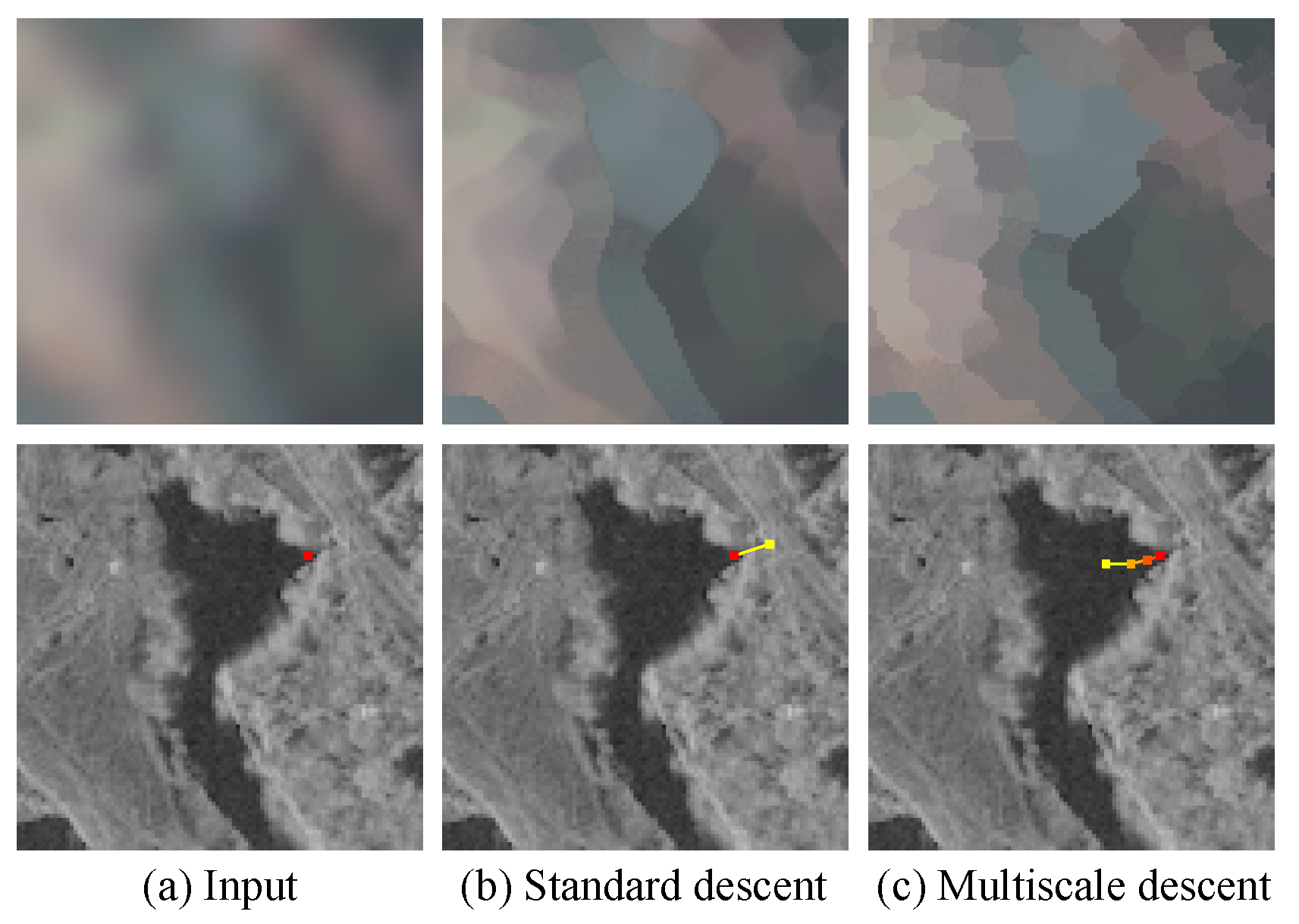
2.3. Multiscale Gradient Descent

Multiscale gradient descent [36] is performed on the upsampled-LR, down-up-sampled-HR, and texture-descriptor images to create their edge-aware versions. Here, “down-up-sampled” means a process composed of low-pass filtering, downsampling, and upsampling to generate a blurred version of the HR image, and “edge” refers to boundaries of objects recognizable in the LR image. The edge-aware LR and down-up-sampled HR images are denoted as $I_{MGD}$ and $J_{MGD}$, respectively. The multiscale gradient descent has two important roles: (1) unmixing boundaries of objects; and (2) dealing with local misregistration between the input LR-HR images, which is always the case for the fusion of multimodal images, such as optical-SAR fusion, LWIR-HS-RGB fusion, and DEM-MS fusion.

Let us consider a blurred LR image and an HR guidance image. The multiscale gradient descent transfers edges in the guidance image into the blurred LR image for objects (or structures) recognizable in the LR image. Figure 2 illustrates the gradient descent and the multiscale gradient descent using the color and SAR images for the blurred LR and HR guidance images, respectively. The gradient descent replaces the pixel values of the LR image around the edges in the HR image with those of more homogeneous neighboring pixels (see Figure 2b). The gradient is calculated using a blurred version of the gradient magnitude image of the HR guidance image. A blurring scale can be defined by the GSD ratio. If the GSD ratio between the LR-HR images is large, some pixel values may not be replaced by those of correct objects because complex transitions between different objects are smoothed out (e.g., the water’s edge in the color image of Figure 2b). To overcome this issue, the multiscale gradient descent is effective by iteratively performing the gradient descent while gradually blurring the HR guidance image at a larger scale [36]. In Figure 2c, we can see that the complex water’s edge is aware in the color image. In this work, a Gaussian filter is used for blurring, where its full width at half maximum (FWHM) is set to two to the GSD ratio between the input LR-HR images for the second- and higher-scale gradient descent procedures, respectively.

2.4. Texture-Guided Filtering

This paper proposes texture-guided filtering as a new intensity modulation technique to transfer spatial details in the HR image to the LR image. At each target pixel, its high-frequency component is obtained via a texture-guided version of MRA where the high-level (low-resolution) components are calculated by weighted summation of neighborhood pixel values in the edge-aware images (i.e., $I_{MGD}$ and $J_{MGD}$) obtained by the previous step. Texture-guided filtering is defined as

$$I_{\mathrm{filtered}}\left(\mathbf{p}\right)=\frac{J\left(\mathbf{p}\right){\sum }_{{\mathbf{p}}_i\in {\Omega }_R}{I}_{\mathrm{MGD}}\left({\mathbf{p}}_i\right)g(\mathbf{f}\left({\mathbf{p}}_i\right)-\mathbf{f}\left(\mathbf{p}\right))}{{\sum }_{{\mathbf{p}}_i\in {\Omega }_R}{J}_{\mathrm{MGD}}\left({\mathbf{p}}_i\right)g(\mathbf{f}\left({\mathbf{p}}_i\right)-\mathbf{f}\left(\mathbf{p}\right))}$$

(4)

where $I_{\mathrm{filtered}}$ is the filtered image and J is the transformed HS image. ${\Omega }_R$ is the $(2R+1)\times (2R+1)$ window centered at $\mathbf{p}$, $g\left(\mathbf{y}\right)=exp\left(\frac{-\parallel \mathbf{y}\parallel }{2{\sigma }^2}\right)$ is the texture kernel for smoothing differences in texture descriptors, and $\sigma$ controls how many of the neighboring pixels having similar textures are considered when obtaining the pixel values of the high-level image in MRA. R is set to be the GSD ratio. Similar to smoothing filtered-based intensity modulation (SFIM) [7], the proposed method assumes that the ratio of pixel values between an image to be estimated ($I_{\mathrm{filtered}}$) and its high-level image is proportional to that between the transformed HS image (J) and the corresponding high-level image. The edge-aware LR image ($I_{\mathrm{MGD}}$) and the edge-aware down-up-sampled HR image ($J_{\mathrm{MGD}}$) are used to calculate the high-level components in MRA with weighting factors for neighboring pixels based on texture similarity. Neighboring pixels (${\mathbf{p}}_i\in \Omega$) are taken into account for obtaining the high-level components to cope with misregistration between the two input images. If the two input images can be co-registered accurately (e.g., pan-sharpening and HS-MS fusion), TGMS directly uses $I_{\mathrm{MGD}}$ and $J_{\mathrm{MGD}}$ for the high-level components, and therefore, Equation (4) can be simplified as $I_{\mathrm{filtered}}\left(\mathbf{p}\right)=J\left(\mathbf{p}\right)I_{\mathrm{MGD}}\left(\mathbf{p}\right)/J_{\mathrm{MGD}}\left(\mathbf{p}\right)$.

3. Evaluation Methodology

3.1. Three Evaluation Scenarios

The experimental part (Section 4 and Section 5) presents six different types of multisensor superresolution problems under three different evaluation scenarios, namely, synthetic, semi-real, and real data evaluation depending on the availability of data sets (see

Table 2. Evaluation scenarios and quality indices used for six specific fusion problems under investigation.

Coarse Category	Optical Data Fusion			Multimodal Data Fusion
Fusion problem	MS-PAN	HS-PAN	HS-MS	Optical-SAR	LWIR-HS-RGB	DEM-MS
Evaluation scenario	Semi-real	Synthetic	Synthetic	Real	Real	Semi-real
Quality indices	PSNR, SAM, ERGAS, $Q{2}^n$			—	—	Q index

). The characteristics of the three evaluation scenarios are summarized in the following subsections.

3.1.1. Synthetic Data Evaluation

Two input images are synthesized from the same data source by degrading it via simulated observations. The reference image is available and, therefore, the synthetic data evaluation is suitable for assessing the performance of spatial resolution enhancement quantitatively. This evaluation procedure is known as Wald’s protocol in the community [39]. The input images are very ideal. For example, in the case of HS-MS fusion, simplified data acquisition simulations that take into account sensor functions and noise are often used in the literature [25], and there is no mismatch between the input images due to errors in the data processing chain, including radiometric, geometric, and atmospheric correction. As a result, the performance of spatial resolution enhancement is likely to be overvalued compared with that for semi-real or real data. Realistic simulations are required to evaluate the robustness of fusion algorithms against various residuals contained in the input images [40]. In this paper, versions of Wald’s protocol presented in [25,41] are adopted for the quantitative assessment of HS pan-sharpening and HS-MS fusion, respectively.

3.1.2. Semi-Real Data Evaluation

Two input images are synthesized from the different data sources using degradation simulations. The HR image is degraded spatially to the same (or lower) resolution as the original LR image. If the original images have the same spatial resolution, only the one for the LR image is degraded spatially. The original LR image is used as the reference image, and the quantitative assessment is feasible at the target spatial resolution. The semi-real data evaluation is widely used in the pan-sharpening community [3]. Since the original data sources are acquired by different imaging sensors, they potentially include real mismatches between the input images. Therefore, the performance of spatial resolution enhancement can be evaluated in more realistic situations than the synthetic data evaluation.

3.1.3. Real Data Evaluation

Two images are acquired from different sensors and directly used as the input of data fusion. Since there is no HR reference image, the quantitative assessment of fused data at the target spatial resolution is not possible. In the pan-sharpening community, the standard technique for quantitative quality assessment of real data is to investigate consistency between the input images and degraded versions of the fused image using quality indices [42]. The quality with no reference index [43] has been widely used as another alternative. If there is any mismatch between the input images, which is always the case in multimodal data fusion, the fused image is either biased to one of them or intermediate. Therefore, an objective numerical comparison is very challenging and visual assessment takes on an important role.

3.2. Quality Indices

Four well-established quality indices are used for the quantitative assessment of multisensor superresolution with synthetic and semi-real data: (1) peak signal-to-noise ratio (PSNR); (2) spectral angle mapper (SAM); (3) erreur relative globale adimensionnelle de synthèse (ERGAS); (4) $Q{2}^n$. This section briefly describes these indices.

Let $\mathbf{X}\in {\mathbb{R}}^{B\times P}$ denote the reference image with B bands and P pixels. $\mathbf{X}={[{\mathbf{x}}_1,...,{\mathbf{x}}_B]}^T=[{\mathbf{x}}_1,...,{\mathbf{x}}_P]$, where ${\mathbf{x}}_i\in {\mathbb{R}}^{P\times 1}$ is the ith band ($i=1,...,B$) and ${\mathbf{x}}_j\in {\mathbb{R}}^{B\times 1}$ is the feature vector of the jth pixel ($j=1,...,P$). $\widehat{\mathbf{X}}$ denotes the estimated image.

3.2.1. PSNR

PSNR qualifies the spatial reconstruction quality of reconstructed images. PSNR is defined as the ratio between the maximum power of a signal and the power of residual errors. The PSNR of the ith band is defined as

$$\mathrm{PSNR}({\mathbf{x}}_i,{\widehat{\mathbf{x}}}_i)=10·{\log }_{10}\left(\frac{\max {\left({\mathbf{x}}_i\right)}^2}{\parallel {\mathbf{x}}_i-{\widehat{\mathbf{x}}}_i{\parallel }_2^2/P}\right),$$

(5)

where $\max \left({\mathbf{x}}_i\right)$ is the maximum pixel value in the ith reference band image. A larger PSNR value indicates a higher quality of spatial reconstruction (for identical data, the PSNR is infinite). If $B>1$, the average PSNR over all bands represents the quality index of the entire image.

3.2.2. SAM

The SAM index [44] is widely used to assess the spectral information preservation at each pixel. SAM determines the spectral distortion by calculating the angle between two vectors of the estimated and reference spectra. The SAM index at the jth pixel is defined as

$$\mathrm{SAM}({\mathbf{x}}_j,{\widehat{\mathbf{x}}}_j)=\arccos \left(\frac{{\mathbf{x}}_j^T{\widehat{\mathbf{x}}}_j}{\parallel {\mathbf{x}}_j{\parallel }_2{\parallel {\widehat{\mathbf{x}}}_j\parallel }_2}\right).$$

(6)

The best value is zero. The average SAM value over all pixels represents the quality index of the entire image.

3.2.3. ERGAS

ERGAS is a global statistical measure of the quality of the resolution-enhanced image [45] with the best value at 0. ERGAS is defined as

$$\mathrm{ERGAS}(\mathbf{X},\widehat{\mathbf{X}})=100d\sqrt{\frac{1}{B}\sum _{i=1}^B\frac{\parallel {\mathbf{x}}_i-{\widehat{\mathbf{x}}}_i{\parallel }_2^2}{{\left(\frac{1}{P}{\mathbf{1}}_P^T{\mathbf{x}}_i\right)}^2}},$$

(7)

where d is the GSD ratio defined as $d=\sqrt{\frac{P_l}{P}}$, $P_l$ is the number of pixels of the LR image, and ${\mathbf{1}}_P={[1,...,1]}^T\in {\mathbb{R}}^{P\times 1}$. ERGAS is the band-wise normalized root-mean-square error multiplied by the GSD ratio to take the difficulty of the fusion problem into consideration.

3.2.4. $Q{2}^n$

The $Q{2}^n$ index [46] is a generalization of the universal image quality index (UIQI) [47] and an extension of the $Q4$ index [35] to spectral images based on hypercomplex numbers. Wang and Bovik proposed the UIQI (or the Q index) [47] to measure any image distortion as the product of three factors: loss of correlation, luminance distortion, and contrast distortion. The UIQI between the reference image ($\mathbf{x}$) and the target image ($\mathbf{y}$) is defined as

$$\mathrm{Q}(\mathbf{x},\mathbf{y})=\frac{{\sigma }_{xy}}{{\sigma }_x{\sigma }_y}\frac{2\overline{x}\overline{y}}{{\overline{x}}^2+{\overline{y}}^2}\frac{2{\sigma }_x{\sigma }_y}{{\sigma }_x^2+{\sigma }_y^2}$$

(8)

where $\overline{x}=\frac{1}{P}{\sum }_{j=1}^P{x}_j$, $\overline{y}=\frac{1}{P}{\sum }_{j=1}^P{y}_j$, ${\sigma }_x=\sqrt{\frac{1}{P}{\sum }_{j=1}^P{(x_j-\overline{x})}^2}$, ${\sigma }_y=\sqrt{\frac{1}{P}{\sum }_{j=1}^P{(y_j-\overline{y})}^2}$, and ${\sigma }_{xy}=\frac{1}{P}{\sum }_{j=1}^P(x_j-\overline{x})(y_j-\overline{y})$. The three components in Equation (8) correspond to correlation, luminance distortion, and contrast distortion, respectively. UIQI has been designed for monochromatic images. To take into account spectral distortion additionally, the $Q4$ index has been developed for four-band images based on modeling each pixel spectrum as a quaternion [35]. $Q{2}^n$ further extends the $Q4$ index by modeling each pixel spectrum (${\mathbf{x}}_j$) as a hypercomplex number, namely a $2^n$-ons represented as

$${\mathbf{x}}_j=x_{j,0}+x_{j,1}{i}_1+x_{j,2}{i}_2+...+x_{j,2^n-1}{i}_{2^n-1}.$$

(9)

$Q{2}^n$ can be computed by using the hypercomplex correlation coefficient, which jointly quantifies spectral and spatial distortions [46].

4. Experiments on Optical Data Fusion

The proposed methodology is applied to the following three optical data fusion problems, namely, MS pan-sharpening, HS pan-sharpening, and HS-MS fusion. The fusion results are evaluated both visually and quantitatively using quality indices.

4.1. Data Sets

4.1.1. MS Pan-Sharpening

Two semi-real MS-PAN data sets were simulated from WorldView-3 images. Brief descriptions of the two data sets are given below.

• WorldView-3 Sydney: This data set was acquired by the visible and near-infrared (VNIR) and PAN sensors of WorldView-3 over Sydney, Australia, on 15 October 2014. (Available Online: https://www.digitalglobe.com/resources/imagery-product-samples/standard-satellite-imagery). The MS image has eight spectral bands in the VNIR range. The GSDs of the MS-PAN images are 1.6 m and 0.4 m, respectively. The study area is a 1000 × 1000 pixel size image at the resolution of the MS image, which includes parks and urban areas.
• WorldView-3 Fukushima: This data set was acquired by the VNIR and PAN sensors of WorldView-3 over Fukushima, Japan, on 10 August 2015. The MS image has eight spectral bands in the VNIR range. The GSDs of the MS-PAN images are 1.2 m and 0.3 m, respectively. The study area is a 1000×1000 pixel size image at the resolution of the MS image taken over a town named Futaba.

MS-PAN data sets are simulated based on the semi-real data evaluation in Section 3.1.2. Spatial simulation is performed to generate the LR versions of the two images using an isotropic Gaussian point spread function (PSF) with an FWHM of the Gaussian function equal to the downscaling factor. For each data set, two synthetic data sets with different GSD ratios (four and eight) were simulated. A GSD of eight was considered for two reasons: (1) to investigate the robustness of the proposed method against the GSD ratio; (2) to conduct parameter sensitivity analysis with different GSD ratios in Section 4.2.4.

4.1.2. HS Pan-Sharpening

Two synthetic HS-PAN data sets were simulated from airborne HS images. Brief descriptions of the two data sets are given below.

• ROSIS-3 University of Pavia: This data was acquired by the reflective optics spectrographic imaging system (ROSIS-3) optical airborne sensor over the University of Pavia, Italy, in 2003. A total of 103 bands covering the spectral range from 0.430 to 0.838 $\mathsf{\mu }$m are used in the experiment after removing 12 noisy bands. The study scene is a 560 × 320 pixel size image with a GSD of 1.3 m.
• Hyperspec-VNIR Chikusei: The airborne HS data set was taken by Headwall’s Hyperspec-VNIR-C imaging sensor over agricultural and urban areas in Chikusei, Ibaraki, Japan, on 19 July 2014. The data set comprises 128 bands in the spectral range from 0.363 to 1.018 $\mathsf{\mu }$m. The study scene is a 540 × 420 pixel size image with a GSD of 2.5 m. More detailed descriptions regarding the data acquisition and processing are given in [48].

HS-PAN data sets are simulated using a version of Wald’s protocol presented in [25]. The PAN image is created by averaging all bands of the original HS image, assuming a uniform spectral response function for simplicity. Spatial simulation is performed to generate the LR-HS image using an isotropic Gaussian PSF with an FWHM of the Gaussian function equal to the GSD ratio between the input HS-PAN images. A GSD ratio of five is used for both data sets.

4.1.3. HS-MS Data Fusion

Two synthetic HS-MS data sets are simulated from HS images taken by the airborne visible/infrared imaging spectrometer (AVIRIS). Brief descriptions of the two HS images are given below.

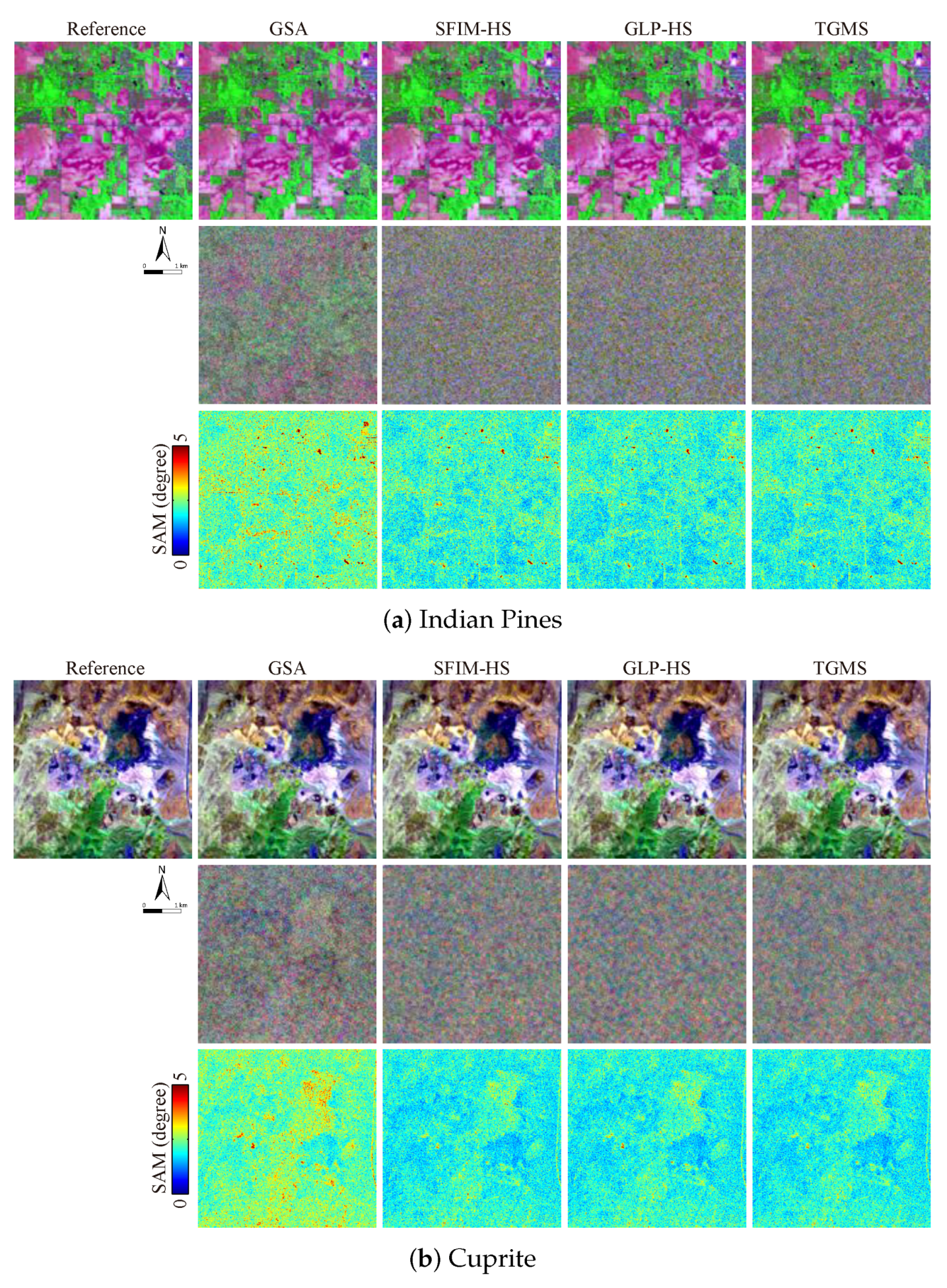
• AVIRIS Indian Pines: This HS image was acquired by the AVIRIS sensor over the Indian Pines test site in northwestern Indiana, USA, in 1992 [49]. The AVIRIS sensor acquired 224 spectral bands in the wavelength range from 0.4 to 2.5 $\mathsf{\mu }$m with an FWHM of 10 nm. The image consists of 512 × 614 pixels at a GSD of 20 m. The study area is a 360 × 360 pixel size image with 192 bands after removing bands of strong water vapor absorption and low SNRs.
• AVIRIS Cuprite: This data set was acquired by the AVIRIS sensor over the Cuprite mining district in Nevada, USA, in 1995. (Available Online: http://aviris.jpl.nasa.gov/data/free_data.html). The entire data set comprises five reflectance images and this study used one of them saved in the file named f970619t01p02_r02_sc03.a.rfl. The full image consists of 512 × 614 pixels at a GSD of 20 m. The study area is a 420 × 360 pixel size image with 185 bands after removing noisy bands.

HS-MS data sets are simulated using a version of Wald’s protocol presented in [41]. Spectral simulation is performed to generate the MS image by degrading the reference image in the spectral domain, using the spectral response functions of WorldView-3 as filters. Spatial simulation is carried out to generate the LR-HS image using an isotropic Gaussian PSF with an FWHM of the Gaussian function equal to the GSD ratio between the input HS-MS images. GSD ratios of six and five are used for the Indian Pines and Cuprite data sets, respectively. After spectral and spatial simulations, band-dependent Gaussian noise was added to the simulated HS-MS images. For realistic noise conditions, an SNR of 35 dB was simulated in all bands.

4.2. Results

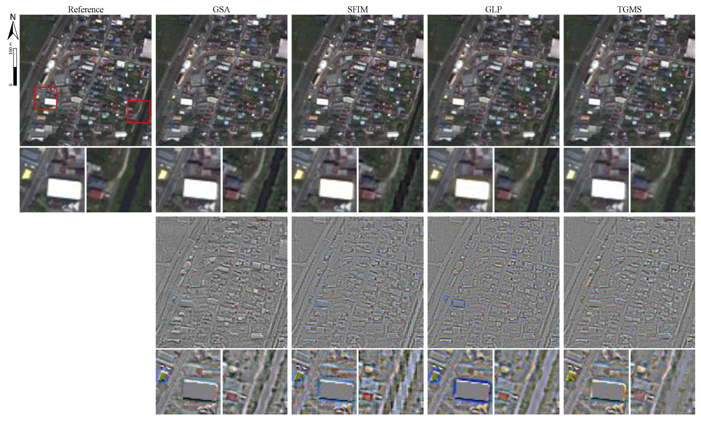
4.2.1. MS Pan-Sharpening

The proposed method is compared with three benchmark pan-sharpening methods—namely, Gram-Schmidt adaptive (GSA) [6], SFIM [7], and generalized Laplacian pyramid (GLP) [8]. GSA is based on component substitution, and SFIM and GLP are MRA-based methods. GSA and GLP showed great and stable performance for various data sets in a recent comparative study in [3].

The upper images in Figure 3 show the color composite images of the reference and pan-sharpened images for the Fukushima data set with a GSD ratio of four. The lower images in Figure 3 present the error images of color-composites relative to the reference after contrast stretching, where gray pixels mean no error and colored pixels indicate local spectral distortion. From the enlarged images, we observe that TGMS mitigates errors in boundaries of objects. For instance, blurring and mixing effects are visible around bright buildings in the results of GLP, whereas the proposed method reduces such artifacts. In the third enlarged images of the WorldView-3 Fukushima data set for GSA, SFIM, and GLP, artifacts can be seen in the stream: the center of the stream is bright while its boundaries with grass regions are dark. TGMS overcomes these artifacts and shows visual results similar to the reference image.

Table 3. Quality indices for WorldView-3 Sydney and Fukushima Data Sets.

Data Set	WorldView-3 Sydney
GSD Ratio	4				8
Method	PSNR	SAM	ERGAS	$\mathit{Q}\mathbf{8}$	PSNR	SAM	ERGAS	$\mathit{Q}\mathbf{8}$
GSA	30.5889	7.0639	4.8816	0.84731	29.5442	8.9376	2.7818	0.80189
SFIM	30.284	7.4459	4.9078	0.80717	29.0397	9.3161	2.8346	0.75794
GLP	30.0165	7.5339	5.0067	0.819	28.634	9.7685	2.9399	0.76188
TGMS	30.5383	7.061	4.8447	0.84063	29.3084	8.8521	2.7895	0.79366
Data Set	WorldView-3 Fukushima
GSD Ratio	4				8
Method	PSNR	SAM	ERGAS	$\mathit{Q}\mathbf{8}$	PSNR	SAM	ERGAS	$\mathit{Q}\mathbf{8}$
GSA	35.2828	3.5409	2.1947	0.86497	32.6051	5.3814	1.5341	0.7814
SFIM	34.4099	3.5878	2.2865	0.82623	31.9744	5.1626	1.5426	0.7534
GLP	34.9059	3.4938	2.162	0.84492	32.1053	5.2448	1.5273	0.76752
TGMS	35.2873	3.2785	2.0986	0.86442	32.5916	4.9253	1.4623	0.78618

summarizes the quality indices obtained by all methods under comparison for both data sets with the two cases of the GSD ratio. TGMS shows the best or second-best indices for all pan-sharpening problems. In particular, the proposed method demonstrates the advantage in the spectral quality measured by SAM. Although the differences of SAM values between TGMS and the other methods are small, they are statistically significant as the p-values of the two-sided Wilcoxon rank sum test for SAM values are all much less than $0.05$. Furthermore, TGMS shows robust performance against the GSD ratio. In general, the quality of pan-sharpened images decreases as the GSD ratio increases, as shown in Table 3. The performance degradation of TGMS is smaller than those of the other methods for most of the indices. Note that all data sets include misregistration between the MS and PAN images due to the different imaging systems. GSA shows the best results in some indices because of its higher robustness against misregistration than MRA-based algorithms [2].

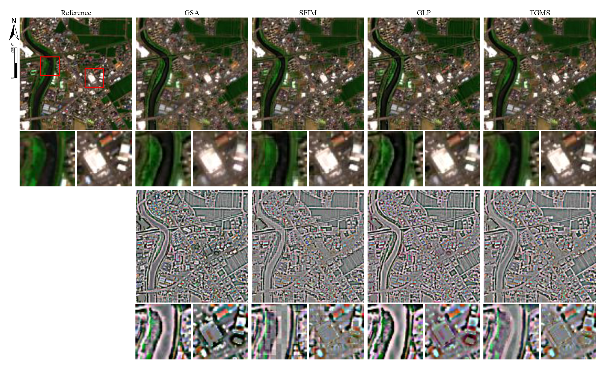
4.2.2. HS Pan-Sharpening

Like the pan-sharpening experiments, the proposed method is compared with GSA, SFIM, and GLP. GLP was one of the high-performance methods in a recent review paper on HS pan-sharpening, followed by SFIM and GSA [25].

Figure 4 shows the visual results for the Hyperspec-VNIR Chikusei data set: the color composite images of the reference and pan-sharpened images in the upper and the color-composite error images in the lower. Similar to the results of pan-sharpening, errors in boundaries of objects obtained by TGMS are smaller than those of the other methods, as can be seen in the enlarged color-composite error images. For instance, the advantage of TGMS is observed in the boundaries of the stream and the white buildings in the first and second enlarged images, respectively.

Table 4. Quality indices for ROSIS-3 University of Pavia and Hyperspec-VNIR Chikusei Data Sets.

	ROSIS University of Pavia				Hyperspec-VNIR Chikusei
Method	PSNR	SAM	ERGAS	Q${\mathbf{2}}^{\mathit{n}}$	PSNR	SAM	ERGAS	Q${\mathbf{2}}^{\mathit{n}}$
GSA	31.085	6.8886	3.6877	0.63454	33.8284	6.9878	4.7225	0.81024
SFIM	31.0686	6.7181	3.6715	0.60115	34.5728	6.409	4.3559	0.84793
GLP	31.6378	6.5862	3.4586	0.6462	33.9539	7.201	4.6249	0.81834
TGMS	31.8983	6.2592	3.3583	0.6541	35.3262	6.1197	4.0381	0.86051

summarizes the quality indices obtained by all methods under comparison for both data sets. TGMS clearly outperforms the other methods for both problems, showing the best results in all indices. The advantage of TGMS over the comparison methods in the quantitative assessment is larger than that observed in the MS pan-sharpening experiments.

4.2.3. HS-MS Fusion

The proposed method is compared with three HS-MS fusion methods based on GSA, SFIM, and GLP, respectively. GSA is applied to HS-MS fusion by constructing multiple image sets for pan-sharpening subproblems where each set is composed of one MS band and corresponding HS bands grouped by correlation-based analysis. SFIM and GLP are adapted to HS-MS fusion by hypersharpening, which synthesizes an HR image for each HS band using a linear regression of MS bands via least squares methods [31]. Here, these two methods are referred to as SFIM-HS and GLP-HS.

Figure 5 presents visual results for the two data sets. All methods considered in this paper show good visual results, and it is hard to visually discern the differences between the reference and fused images from the color composites. The errors of the fusion results are visualized by differences of color composites (where gray pixels mean no fusion error and colored pixels indicate local spectral distortion) and SAM images. The results of TGMS are very similar to those of SFIM-HS and GLP-HS.

Table 5. Quality indices for AVIRIS Indian Pines and Cuprite Data Sets.

	AVIRIS Indian Pines				AVIRIS Cuprite
Method	PSNR	SAM	ERGAS	Q${\mathbf{2}}^{\mathit{n}}$	PSNR	SAM	ERGAS	Q${\mathbf{2}}^{\mathit{n}}$
GSA	40.0997	0.96775	0.44781	0.95950	39.2154	0.98265	0.37458	0.98254
SFIM-HS	40.7415	0.84069	0.40043	0.91297	40.8674	0.79776	0.31375	0.97017
GLP-HS	41.2962	0.82635	0.37533	0.95236	40.8240	0.80250	0.31570	0.97838
TGMS	40.8867	0.83001	0.39279	0.9187	40.9704	0.78922	0.30984	0.97852

shows the quality indices obtained by all methods under comparison for both data sets. TGMS demonstrates comparable or better results for both data sets compared to those of the other methods. More specifically, PSNR, SAM, and ERGAS values obtained by the proposed method are the second-best for the Indian Pines data set, while these values are the best for the Cuprite data set.

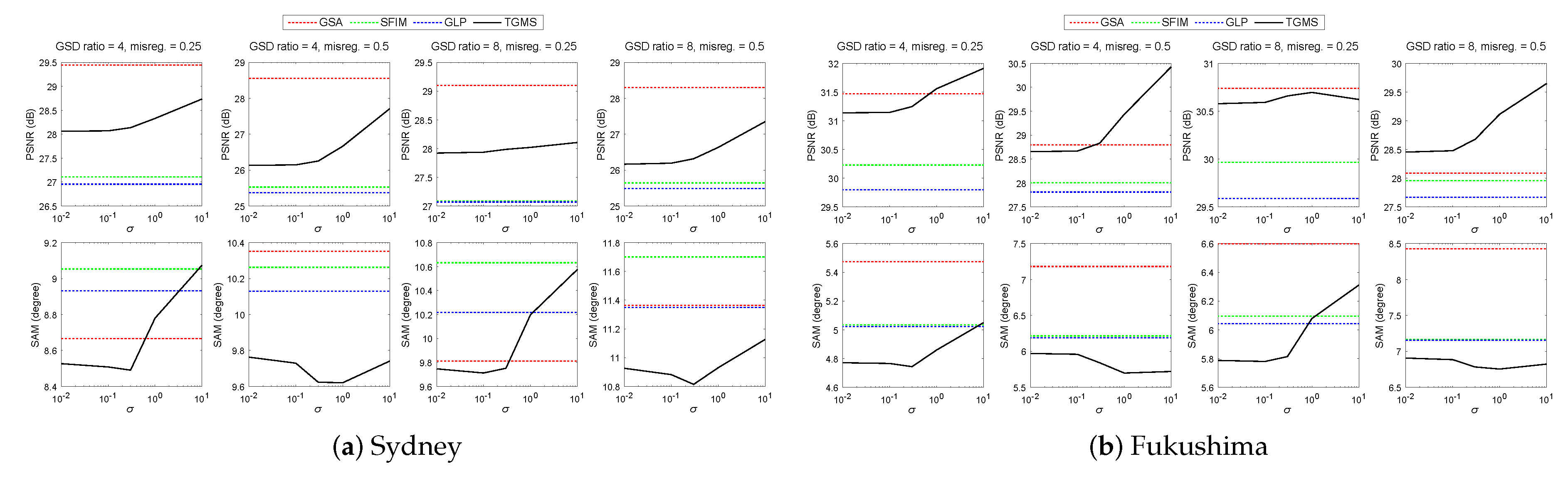
4.2.4. Parameter Sensitivity Analysis

In Section 4.2.1 and Section 4.2.2, since the input MS-PAN images are co-registered well, the simplified version of texture-guided filtering was used as mentioned in Section 2.4. If there is any misregistration between the input images, the parameter $\sigma$ is the most important parameter for the proposed method. Here, we analyze the sensitivity of TGMS to the change of $\sigma$ in case the input images are not accurately co-registered, using pan-sharpening problems as examples. Two cases of global misregistration, namely, 0.25 and 0.5 pixels in the lower resolution, are simulated for both data sets with the two scenarios of the GSD ratio.

Figure 6a,b plots the PSNR and SAM performance as a function of $\sigma$ under four different scenarios for the WorldView-3 Sydney and Fukushima data sets, respectively. We can observe the optimal range of $\sigma$ for the maximum SAM value of each pan-sharpening problem. When $\sigma$ increases, there is a trade-off between the spatial and spectral quality: both PSNR and SAM increase. Considering the optimal range of $\sigma$ for SAM and the trade-off between PSNR and SAM regarding $\sigma$, we found that the range of $0.1\le \sigma \le 1$ is effective for dealing with misregistration.

5. Experiments on Multimodal Data Fusion

This section demonstrates applications of the proposed methodology to three multimodal data fusion problems: optical-SAR fusion, LWIR-HS-RGB fusion, and DEM-MS fusion. The parameter $\sigma$ was set to be $0.3$ according to the parameter sensitivity analysis in Section 4.2.3. The fusion results are qualitatively validated.

5.1. Data Sets

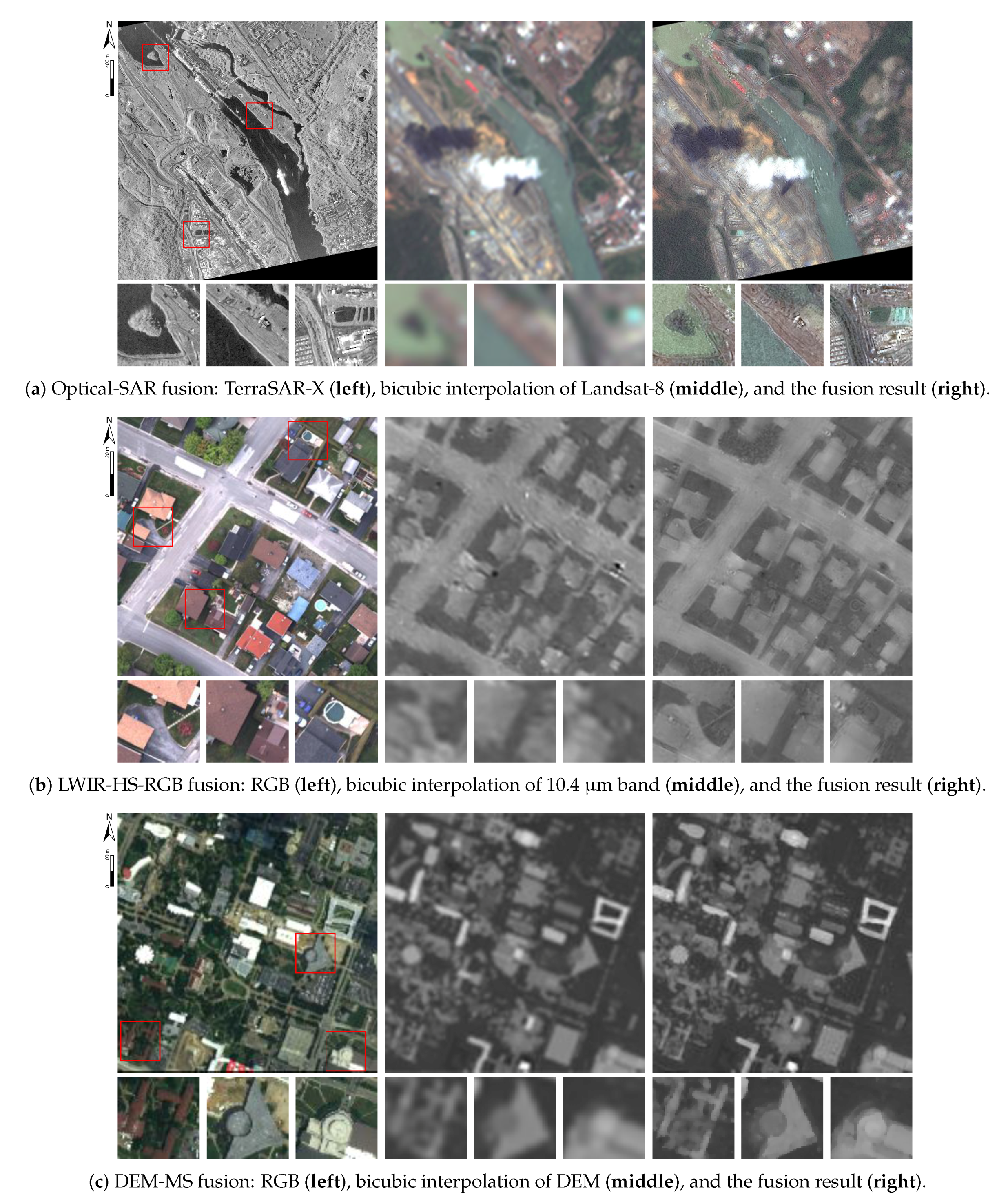
• Optical-SAR fusion: This data set is composed of Landsat-8 and TerraSAR-X images taken over the Panama Canal, Panama. The Landsat-8 image was acquired on 5 March 2015. Bands 1–7 at a GSD of 30 m are used for the LR image of multisensor superresolution. The TerraSAR-X image was acquired with the sparing spotlight mode on 12 December 2013, and distributed as the enhanced ellipsoid corrected product at a pixel spacing of 0.24 m. (Available Online: http://www.intelligence-airbusds.com/en/23-sample-imagery). To reduce the speckle noise, the TerraSAR-X image was downsampled using a Gaussian filter for low-pass filtering so that the pixel spacing is equal to 3 m. The study area is a 1000 × 1000 pixel size image at the higher resolution. The backscattering coefficient is used for the experiment.
• LWIR-HS-RGB fusion: This data set comprises LWIR-HS and RGB images taken over an urban area near Thetford Mines in Québec, Canada, simultaneously on 21 May 2013. The data set was provided for the IEEE 2014 Geoscience and Remote Sensing Society (GRSS) Data Fusion Contest by Telops Inc. (Québec, QC, Canada) [50]. The LWIR-HS image was acquired by the Hyper-Cam, which is an airborne LWIR-HS imaging sensor based on a Fourier-transform spectrometer, with 84 bands covering the wavelengths from 7.8 to 11.5 $\mathsf{\mu }$m at a GSD of 1 m. The RGB image was acquired by a digital color camera at a GSD of 0.2 m. The study area is a 600 × 600 pixel size image at the higher resolution. There is a large degree of local misregistration (more than one pixel in the lower resolution) between the two images. The LWIR-HS image was registered to the RGB image by a projective transformation with manually selected control points.
• DEM-MS fusion: The DEM-MS data set was simulated using LiDAR-derived DEM and HS data taken over the University of Houston and its surrounding urban areas. The original data set was provided for the IEEE 2013 GRSS Data Fusion Contest [51]. The HS image has 144 spectral bands in the wavelength range from 0.4 to 1.0 $\mathsf{\mu }$m with an FWHM of 5 nm. Both images consist of 349 × 1905 pixels at a GSD of 2.5 m. The study area is a 344 × 500 pixel size image mainly over the campus of the University of Houston. To set a realistic problem, only four bands in the wavelengths of 0.46, 0.56, 0.66, and 0.82 $\mathsf{\mu }$m of the HS image are used as the HR-MS image. The DEM is degraded spatially using filtering and downsampling. Filtering was performed using an isotropic Gaussian PSF with an FWHM of the Gaussian function equal to the GSD ratio, which was set to four.

5.2. Results

In Figure 7a, the SAR image and the color composite images of interpolated MS and fused data are shown from left to right. Spatial details obtained from the SAR image are added to the MS data while keeping natural colors (spectral information). The fused image inherits mismatches between the two input images (e.g., clouds and their shadows in the MS image and the ship in the SAR image). Note that speckle noise will be problematic if a lower-resolution SAR image (e.g., TerraSAR-X StripMap data) is used for the HR data source; thus, despeckling plays a critical role [35].

Figure 7b presents the RGB image, the interpolated 10.4 $\mathsf{\mu }$m band of the input LWIR-HS data, and that of the resolution-enhanced LWIR-HS data from left to right. The resolution-enhancement effect can be clearly observed particularly from the enlarged images. Small objects that cannot be recognized in the RGB image are smoothed out (e.g., black spots in the input LWIR-HS image).

In Figure 7c, the color composite of the MS image, the interpolated DEM, and the resolution-enhanced DEM are shown from left to right. It can be seen that the edges of buildings are sharpened. Some artifacts can also be observed. For instance, the elevation of pixels corresponding to cars in the parking lot located south of the triangular building (shown in the second enlarged image) is overestimated. The Q index of the resolution-enhanced DEM is 0.9011, whereas those of interpolated DEMs using nearest neighbor and bicubic interpolation are 0.8787 and 0.9009, respectively. The difference in the Q index between the result of TGMS and the interpolated ones is not large, even though the result of TGMS clearly demonstrates the resolution-enhancement effect. This result is due to local misregistration between the original DEM and HS images. The interpolated DEMs are spatially consistent with the reference DEM, whereas the fused DEM is spatially biased to the input MS image.

6. Discussion

This paper proposed a new methodology for multisensor superresolution. The author’s attention was concentrated on establishing a methodology that is applicable to various multisensor superresolution problems, rather than focusing on a specific fusion problem to improve reconstruction accuracy. The originality of the proposed technique lies in its high general versatility.

The experiments on six different types of fusion problems showed the potential of the proposed methodology for various multisensor superresolution tasks. The high general versatility of TGMS is achieved based on two concepts.

The first concept is, if the LR image has multiple bands, to preserve the shapes of the original feature vectors for the resolution-enhanced image by creating new feature vectors as linear combinations of those at local regions in the input LR image, while spatial details are modulated by scaling factors. This concept was inspired by intensity modulation techniques (e.g., SFIM [7]) and bilateral filtering [52]. The effectiveness of the first concept was evidenced by the high spectral performance of TGMS in the experiments on optical data fusion. TGMS does not generate artifacts having unrealistic shapes of feature vectors even in the case of multimodal data fusion owing to this concept.

The second concept is to improve the robustness against spatial mismatches (e.g., local misregistration and GSD ratio) between input images by exploiting spatial structures and image textures in the HR image via MGD and texture-guided filtering. In the case of multimodal data fusion, local misregistration is very troublesome as discussed in the context of image registration [53]. The experimental results on multimodal data fusion implied that this problem could be handled by TGMS owing to the second concept.

In the experiments on optical data fusion, TGMS showed comparable or superior results in both quantitative evaluation and visual evaluation compared with the benchmark techniques. In particular, the proposed method clearly outperformed the other algorithms in HS pan-sharpening. This finding suggests that the concepts mentioned above are suited to the problem setting of HS pan-sharpening, where we need to minimize spectral distortions and avoid spatial over- or under-enhancement. These results are in good agreement with other studies which have shown that a vector modulation-based technique is useful for HS pan-sharpening [54].

The proposed method was assessed mainly by visual analysis for multimodal data fusion because there is no benchmark method and also no evaluation methodology has been established. The visual results of multimodal data fusion suggested a possible beneficial effect of TGMS sharpening boundaries of objects recognizable in the LR image using spatial structures and image textures. Note that the results of multimodal data fusion are not conclusive and its evaluation methodology remains an open issue. TGMS assumes proportionality of pixel values between the two input images after data transformation of the HR image. The main limitation of the proposed method is that spatial details at each object level can include artifacts in pixel-wise scaling factors if this assumption does not hold at local regions or objects. For instance, water regions of the optical-SAR fusion result are noisy as shown in the enlarged images on the right of Figure 7a. If one region is spatially homogeneous or flat, scaling factors for vector modulation can be defined by SNRs. Since water regions in the SAR image have low SNRs, the noise effect was added to the fusion result.

7. Conclusions and Future Lines

This paper proposed a novel technique, namely texture-guided multisensor superresolution (TGMS), for enhancing the spatial resolution of an LR image by fusing it with an auxiliary HR image. TGMS is based on MRA, where the high-level component is obtained taking object structures and HR texture information into consideration. This work presented experiments on six types of multiresolution superresolution problems in remote sensing: MS pan-sharpening, HS pan-sharpening, HS-MS fusion, optical-SAR fusion, LWIR-HS-RGB fusion, and DEM-MS fusion. The quality of the resolution-enhanced images was assessed quantitatively for optical data fusion compared with benchmark methods and also evaluated qualitatively for all problems. The experimental results demonstrated the effectiveness and high versatility of the proposed methodology. In particular, TGMS presented high performance in spectral quality and robustness against misregistration and the resolution ratio, which make it suitable for the resolution enhancement of upcoming spaceborne HS data.

Future work will involve investigating efficient and fast texture descriptors suited to remotely sensed images. Clearly, research on quantitative evaluation methodology for multimodal data fusion is still required.

References

1. Alparone, L.; Wald, L.; Chanussot, J.; Thomas, C.; Gamba, P.; Bruce, L.M. Comparison of pan sharpening algorithms: Outcome of the 2006 GRS-S data fusion contest. IEEE Trans. Geosci. Remote Sens. 2007, 45, 3012–3021. [Google Scholar] [CrossRef]
2. Aiazzi, B.; Alparone, L.; Baronti, S.; Garzelli, A.; Selva, M. 25 years of pansharpening: A critical review and new developments. In Signal Image Processing for Remote Sensing, 2nd ed.; Chen, C.H., Ed.; CRC Press: Boca Raton, FL, USA, 2011; Chapter 28; pp. 533–548. [Google Scholar]
3. Vivone, G.; Alparone, L.; Chanussot, J.; Mura, M.D.; Garzelli, A.; Licciardi, G.; Restaino, R.; Wald, L. A critical comparison among pansharpening algorithms. IEEE Trans. Geosci. Remote Sens. 2015, 53, 2565–2586. [Google Scholar] [CrossRef]
4. Carper, W.; Lillesand, T.M.; Kiefer, P.W. The use of Intensity-Hue-Saturation transformations for merging SPOT panchromatic and multispectral image data. Photogramm. Eng. Remote Sens. 1990, 56, 459–467. [Google Scholar]
5. Laben, C.A.; Brower, B.V. Process for Enhancing the Spatial Resolution of Multispectral Imagery Using Pan-Sharpening. U.S. Patent 6,011,875 A, 4 January 2000. [Google Scholar]
6. Aiazzi, B.; Baronti, S.; Selva, M. Improving component substitution pansharpening through multivariate regression of MS + Pan data. IEEE Trans. Geosci. Remote Sens. 2007, 45, 3230–3239. [Google Scholar] [CrossRef]
7. Liu, J.G. Smoothing Filter-based Intensity Modulation: A spectral preserve image fusion technique for improving spatial details. Int. J. Remote Sens. 2000, 21, 3461–3472. [Google Scholar] [CrossRef]
8. Aiazzi, B.; Alparone, L.; Baronti, S.; Garzelli, A.; Selva, M. MTF-tailored multiscale fusion of high-resolution MS and Pan imagery. Photogramm. Eng. Remote Sens. 2006, 72, 591–596. [Google Scholar] [CrossRef]
9. Pardo-Igúzquiza, E.; Chica-Olmo, M.; Atkinson, P.M. Downscaling cokriging for image sharpening. Remote Sens. Environ. 2006, 102, 86–98. [Google Scholar] [CrossRef]
10. Sales, M.H.R.; Souza, C.M.; Kyriakidis, P.C. Fusion of MODIS images using kriging with external drift. IEEE Trans. Geosci. Remote Sens. 2013, 51, 2250–2259. [Google Scholar] [CrossRef]
11. Wang, Q.; Shi, W.; Atkinson, P.M.; Zhao, Y. Downscaling MODIS images with area-to-point regression kriging. Remote Sens. Environ. 2015, 166, 191–204. [Google Scholar] [CrossRef]
12. Wang, Q.; Shi, W.; Li, Z.; Atkinson, P.M. Fusion of Sentinel-2 images. Remote Sens. Environ. 2016, 187, 241–252. [Google Scholar] [CrossRef]
13. Li, S.; Yang, B. A New Pan-Sharpening Method Using a Compressed Sensing Technique. IEEE Trans. Geosci. Remote Sens. 2011, 49, 738–746. [Google Scholar] [CrossRef]
14. Zhu, X.X.; Bamler, R. A sparse image fusion algorithm With application to pan-sharpening. IEEE Trans. Geosci. Remote Sens. 2013, 51, 2827–2836. [Google Scholar] [CrossRef]
15. He, X.; Condat, L.; Bioucas-Dias, J.M.; Chanussot, J.; Xia, J. A new pansharpening method based on spatial and spectral sparsity priors. IEEE Trans. Image Process. 2014, 23, 4160–4174. [Google Scholar] [CrossRef] [PubMed]
16. Guanter, L.; Kaufmann, H.; Segl, K.; Förster, S.; Rogaß, C.; Chabrillat, S.; Küster, T.; Hollstein, A.; Rossner, G.; Chlebek, C.; et al. The EnMAP spaceborne imaging spectroscopy mission for earth observation. Remote Sens. 2015, 7, 8830–8857. [Google Scholar] [CrossRef]
17. Iwasaki, A.; Ohgi, N.; Tanii, J.; Kawashima, T.; Inada, H. Hyperspectral imager suite (HISUI)—Japanese hyper-multi spectral radiometer. In Proceedings of the IEEE International Geoscience and Remote Sensing Symposium, Vancouver, BC, Canada, 24–29 July 2011; pp. 1025–1028. [Google Scholar]
18. Stefano, P.; Angelo, P.; Simone, P.; Filomena, R.; Federico, S.; Tiziana, S.; Umberto, A.; Vincenzo, C.; Acito, N.; Marco, D.; et al. The PRISMA hyperspectral mission: Science activities and opportunities for agriculture and land monitoring. In Proceedings of the IEEE International Geoscience and Remote Sensing Symposium, Melbourne, VIC, Australia, 21–26 July 2013; pp. 4558–4561. [Google Scholar]
19. Green, R.; Asner, G.; Ungar, S.; Knox, R. NASA mission to measure global plant physiology and functional types. In Proceedings of the IEEE Aerospace Conference, Big Sky, MT, USA, 1–8 March 2008; pp. 1–7. [Google Scholar]
20. Michel, S.; Gamet, P.; Lefevre-Fonollosa, M.J. HYPXIM—A hyperspectral satellite defined for science, security and defense users. In Proceedings of the IEEE Hyperspectral Image and Signal Processing: Evolution in Remote Sensing (WHISPERS), Lisbon, Portugal, 6–9 June 2011; pp. 1–4. [Google Scholar]
21. Eckardt, A.; Horack, J.; Lehmann, F.; Krutz, D.; Drescher, J.; Whorton, M.; Soutullo, M. DESIS (DLR Earth sensing imaging spectrometer for the ISS-MUSES platform. In Proceedings of the IEEE International Geoscience and Remote Sensing Symposium, Milan, Italy, 26–31 July 2015; pp. 1457–1459. [Google Scholar]
22. Feingersh, T.; Dor, E.B. SHALOM—A Commercial Hyperspectral Space Mission. In Optical Payloads for Space Missions; Qian, S.E., Ed.; John Wiley & Sons, Ltd.: Chichester, UK, 2015; Chapter 11; pp. 247–263. [Google Scholar]
23. Chan, J.C.W.; Ma, J.; Kempeneers, P.; Canters, F. Superresolution enhancement of hyperspectral CHRIS/ Proba images with a thin-plate spline nonrigid transform model. IEEE Trans. Geosci. Remote Sens. 2010, 48, 2569–2579. [Google Scholar] [CrossRef]
24. Yokoya, N.; Mayumi, N.; Iwasaki, A. Cross-calibration for data fusion of EO-1/Hyperion and Terra/ASTER. IEEE J. Sel. Top. Appl. Earth Obs. Remote Sens. 2013, 6, 419–426. [Google Scholar] [CrossRef]
25. Loncan, L.; Almeida, L.B.; Dias, J.B.; Briottet, X.; Chanussot, J.; Dobigeon, N.; Fabre, S.; Liao, W.; Licciardi, G.A.; Simões, M.; et al. Hyperspectral pansharpening: A review. IEEE Geosci. Remote Sens. Mag. 2015, 3, 27–46. [Google Scholar] [CrossRef]
26. Yokoya, N.; Grohnfeldt, C.; Chanussot, J. Hyperspectral and multispectral data fusion: A comparative review. IEEE Geosci. Remote Sens. Mag. 2017, in press. [Google Scholar]
27. Eismann, M.T.; Hardie, R.C. Application of the stochastic mixing model to hyperspectral resolution enhancement. IEEE Trans. Geosci. Remote Sens. 2004, 42, 1924–1933. [Google Scholar] [CrossRef]
28. Yokoya, N.; Yairi, T.; Iwasaki, A. Coupled nonnegative matrix factorization unmixing for hyperspectral and multispectral data fusion. IEEE Trans. Geosci. Remote Sens. 2012, 50, 528–537. [Google Scholar] [CrossRef]
29. Simões, M.; Dias, J.B.; Almeida, L.; Chanussot, J. A convex formulation for hyperspectral image superresolution via subspace-based regularization. IEEE Trans. Geosci. Remote Sens. 2015, 53, 3373–3388. [Google Scholar] [CrossRef]
30. Chen, Z.; Pu, H.; Wang, B.; Jiang, G.M. Fusion of hyperspectral and multispectral images: A novel framework based on generalization of pan-sharpening methods. IEEE Geosci. Remote Sens. Lett. 2014, 11, 1418–1422. [Google Scholar] [CrossRef]
31. Selva, M.; Aiazzi, B.; Butera, F.; Chiarantini, L.; Baronti, S. Hyper-sharpening: A first approach on SIM-GA data. IEEE J. Sel. Top. Appl. Earth Obs. Remote Sens. 2015, 8, 3008–3024. [Google Scholar] [CrossRef]
32. Moran, M.S. A Window-based technique for combining Landsat Thematic Mapper thermal data with higher-resolution multispectral data over agricultural land. Photogramm. Eng. Remote Sens. 1990, 56, 337–342. [Google Scholar]
33. Haala, N.; Brenner, C. Extraction of buildings and trees in urban environments. ISPRS J. Photogramm. Remote Sens. 1999, 54, 130–137. [Google Scholar] [CrossRef]
34. Sirmacek, B.; d’Angelo, P.; Krauss, T.; Reinartz, P. Enhancing urban digital elevation models using automated computer vision techniques. In Proceedings of the ISPRS Commission VII Symposium, Vienna, Austria, 5–7 July 2010. [Google Scholar]
35. Alparone, L.; Baronti, S.; Garzelli, A.; Nencini, F. A global quality measurement of pan-sharpened multispectral imagery. IEEE Geosci. Remote Sens. Lett. 2004, 1, 313–317. [Google Scholar] [CrossRef]
36. Arbelot, B.; Vergne, R.; Hurtut, T.; Thollot, J. Automatic texture guided color transfer and colorization. In Proceedings of the Expressive, Lisbon, Portugal, 7–9 May 2016. [Google Scholar]
37. Tuzel, O.; Porikli, F.; Meer, P. A fast descriptor for detection and classification. In Proceedings of the 9th European Conference on Computer Vision, Graz, Austria, 7–13 May 2006; pp. 589–600. [Google Scholar]
38. Karacan, L.; Erdem, E.; Erdem, A. Structure-preserving image smoothing via region covariances. ACM Trans. Graph. 2013, 32, 176:1–176:11. [Google Scholar] [CrossRef]
39. Wald, L.; Ranchin, T.; Mangolini, M. Fusion of satellite images of different spatial resolutions: Assessing the quality of resulting images. Photogramm. Eng. Remote Sens. 1997, 63, 691–699. [Google Scholar]
40. Yokoya, N.; Chan, J.C.W.; Segl, K. Potential of resolution-enhanced hyperspectral data for mineral mapping using simulated EnMAP and Sentinel-2 images. Remote Sens. 2016, 8, 172. [Google Scholar] [CrossRef]
41. Veganzones, M.; Simões, M.; Licciardi, G.; Yokoya, N.; Bioucas-Dias, J.; Chanussot, J. Hyperspectral super-resolution of locally low rank images from complementary multisource data. IEEE Trans. Image Process. 2016, 25, 274–288. [Google Scholar] [CrossRef] [PubMed]
42. Palsson, F.; Sveinsson, J.R.; Ulfarsson, M.O.; Benediktsson, J.A. Quantitative Quality Evaluation of Pansharpened Imagery: Consistency Versus Synthesis. IEEE Trans. Geosci. Remote Sens. 2016, 54, 1247–1259. [Google Scholar] [CrossRef]
43. Alparone, L.; Aiazzi, B.; Baronti, S.; Garzelli, A.; Nencini, F.; Selva, M. Multispectral and panchromatic data fusion assessment without reference. Photogramm. Eng. Remote Sens. 2008, 74, 193–200. [Google Scholar] [CrossRef]
44. Kruse, F.A.; Lefkoff, A.B.; Boardman, J.W.; Heidebrecht, K.B.; Shapiro, A.T.; Barloon, J.P.; Goetz, A.F.H. The spectral image processing system (SIPS)—Interactive visualization and analysis of imaging spectrometer data. Remote Sens. Environ. 1993, 44, 145–163. [Google Scholar] [CrossRef]
45. Wald, L. Quality of High Resolution Synthesised Images: Is There a Simple Criterion? In Proceedings of the Fusion of Earth Data: Merging Point Measurements, Raster Maps and Remotely Sensed Images, Sophia Antipolis, France, 26 January 2000; pp. 99–103. [Google Scholar]
46. Garzelli, A.; Nencini, F. Hypercomplex quality assessment of multi/hyperspectral images. IEEE Geosci. Remote Sens. Lett. 2009, 6, 662–665. [Google Scholar] [CrossRef]
47. Wang, Z.; Bovik, A.C. A universal image quality index. IEEE Signal Process. Lett. 2002, 9, 81–84. [Google Scholar] [CrossRef]
48. Yokoya, N.; Iwasaki, A. Airborne Hyperspectral Data over Chikusei; Technical Report SAL-2016-05-27; Space Application Laboratory, The University of Tokyo: Tokyo, Japan, 2016. [Google Scholar]
49. Baumgardner, M.F.; Biehl, L.L.; Landgrebe, D.A. 220 Band AVIRIS Hyperspectral Image Data Set: June 12, 1992 Indian Pine Test Site 3. Purdue Univ. Res. Repos. 2015. [Google Scholar] [CrossRef]
50. Liao, W.; Huang, X.; Van Coillie, F.; Gautama, S.; Pižurica, A.; Philips, W.; Liu, H.; Zhu, T.; Shimoni, M.; Moser, G.; et al. Processing of multiresolution thermal hyperspectral and digital color data: Outcome of the 2014 IEEE GRSS data fusion contest. IEEE J. Sel. Top. Appl. Earth Obs. Remote Sens. 2015, 8, 2984–2996. [Google Scholar] [CrossRef]
51. Debes, C.; Merentitis, A.; Heremans, R.; Hahn, J.; Frangiadakis, N.; van Kasteren, T.; Liao, W.; Bellens, R.; Piz̆urica, A.; Gautama, S.; et al. Hyperspectral and LiDAR Data Fusion: Outcome of the 2013 GRSS Data Fusion Contest. IEEE J. Sel. Top. Appl. Earth Obs. Remote Sens. 2014, 7, 2405–2418. [Google Scholar] [CrossRef]
52. Tomasi, C.; Manduchi, R. Bilateral filtering for gray and color images. In Proceedings of the IEEE International Conference on Computer Vision, Bombay, India, 4–7 Jaunary 1998; pp. 839–846. [Google Scholar]
53. Suri, S.; Reinartz, P. Mutual-information-based registration of TerraSAR-X and Ikonos imagery in urban areas. IEEE Trans. Geosci. Remote Sens. 2010, 48, 939–949. [Google Scholar] [CrossRef]
54. Garzelli, A.; Capobianco, L.; Alparone, L.; Aiazzi, B.; Baronti, S.; Selva, M. Hyperspectral pansharpening based on modulation of pixel spectra. In Proceedings of the IEEE 2nd Workshop on Hyperspectral Image and Signal Processing: Evolution in Remote Sensing (WHISPERS), Reykjavìk, Iceland, 14–16 June 2010; pp. 1–4. [Google Scholar]
Figure 1. Overview of texture-guided multisensor superresolution in case of optical-SAR fusion.
Remotesensing 09 00316 g001
Figure 2. Illustrations of gradient descent methods.
Remotesensing 09 00316 g002
Figure 3. (Upper) Color composites of reference, GSA, SFIM, GLP, and TGMS images with two enlarged regions from left to right columns, respectively, for 300 × 300 pixels sub-areas of WorldView-3 Fukushima data (©DigitalGlobe). (Lower) Error images relative to the reference data visualized by differences of color composites.
Remotesensing 09 00316 g003
Figure 4. (Upper) Color composites of reference, GSA, SFIM, GLP, and TGMS images with two enlarged regions from left to right columns, respectively, for 300 × 300 pixels sub-areas of Hyperspec-VNIR Chikusei data. (Lower) Error images relative to the reference data visualized by differences of color composites.
Remotesensing 09 00316 g004
Figure 5. HS-MS fusion results for AVIRIS (a) Indian Pines and (b) Cuprite data sets. (1st row) Color composites of reference, GSA, SFIM-HS, GLP-HS, and TGMS images are displayed for a 240 × 240 pixels sub-area. Bands used for red, green, and blue are 2.20, 0.80, and 0.46 μ m for Indian Pines data and 2.20, 1.6, and 0.57 μ m for Cuprite data. Error images relative to the reference data visualized by differences of color composites (2nd row) and SAM images (3rd row).
Remotesensing 09 00316 g005
Figure 6. Sensitivity to the parameter σ measured by PSNR (upper row) and SAM (lower row) for WorldView-3 (a) Sydney and (b) Fukushima data sets. Different columns indicate the results with various combinations of the GSD ratio and the degree (pixel) of misregistration at low resolution.
Remotesensing 09 00316 g006
Figure 7. Multisensor superresolution results. (a) Fusion of MS-SAR images: TerraSAR-X with the staring stoplight mode downsampled at 3-m GSD, bicubic interpolation of Landsat-8 originally at 30-m GSD, and resolution-enhanced Landsat-8 from left to right. (b) Fusion of LWIR-HS-RGB images: RGB at 0.2-m GSD, bicubic interpolation of 10.4 μ m band originally at 1-m GSD, and resolution-enhanced 10.4 μ m band from left to right. (c) Fusion of DEM-MS images: RGB at 2.5-m GSD, bicubic interpolation of DEM originally at 10-m GSD, and resolution-enhanced DEM from left to right.
Remotesensing 09 00316 g007