Fluorescence-Based Approach to Estimate the Chlorophyll-A Concentration of a Phytoplankton Bloom in Ardley Cove (Antarctica)

Abstract

A phytoplankton bloom occurred in Ardley Cove, King George Island in January 2016, during which maximum chlorophyll-a reached 9.87 mg/m³. Records show that blooms have previously not occurred in this area prior to 2010 and the average chlorophyll-a concentration between 1991 and 2009 was less than 2 mg/m³. Given the lack of in situ measurements and the poor performance of satellite algorithms in the Southern Ocean and Antarctic waters, we validate and assess several chlorophyll-a algorithms and apply an improved baseline fluorescence approach to examine this bloom event. In situ water properties including in vivo fluorescence, water leaving radiance, and solar irradiance were collected to evaluate satellite algorithms and characterize chlorophyll-a concentration, as well as dominant phytoplankton groups. The results validated the nFLH fluorescence baseline approach, resulting in a good agreement at this high latitude, high chlorophyll-a region with correlation at 59.46%. The dominant phytoplankton group within the bloom was micro-phytoplankton, occupying 79.58% of the total phytoplankton community. Increasing sea ice coverage and sea ice concentration are likely responsible for increasing phytoplankton blooms in the recent decade. Given the profound influence of climate change on sea-ice and phytoplankton dynamics in the region, it is imperative to develop accurate methods of estimating the spatial distribution and concentrations of the increasing occurrence of bloom events.

1. Introduction

Due to the extreme climate and the difficulties of conducting field research above 60° south, the Southern Ocean (SO), especially around Antarctica, lacks a systematic in situ sampling program of its peculiar bio-optics and micro-organism community structure [1,2,3]. As a result, satellite measurements from space still have large errors in estimating phytoplankton biomass [4,5] and global chlorophyll-a satellite algorithms typically underestimate chlorophyll-a in the Southern Ocean [6,7,8,9,10,11].

There are three main reasons for global algorithm underestimation. First is the difference in optical properties between global and SO waters. Compared with the global ocean, the SO has a narrower water leaving radiance in the green band [12]. This narrow gap leads to underestimation of chlorophyll-a in blue-green band ratio algorithms such as OC3 or OC4 [13,14]. Second, seasonal sea ice causes contaminated pixels, which underestimate chlorophyll-a in > 1.5 mg/m³ and overestimates in < 1.5 mg/m³ waters [15,16]. These are obvious patterns in the Arctic and are probably similar in Antarctica. Third, inappropriate atmospheric correction in the SO introduces error when converting top of atmosphere radiance into the water leaving radiance. The SO has unique aerosols and cloud coverage [17], and lacks a proper vertical atmospheric simulation to correct for aerosol influences [18].

In addition to band-ratio chlorophyll-a algorithms, state-of-the-art algorithms for global chlorophyll-a estimation include IOP (inherent optical property) bio-optical models (e.g., GSM01 [19] and QAA (quasi-analytical algorithm) [20]) and baseline algorithms, such as nFLH (normalized fluorescence line height). Bands setting at 667, 678, and 748 nm help MODIS become the only satellite to achieve the baseline nFLH approach, which estimates chlorophyll-a through fluorescence intensity from photosynthesis products [21].

$$\mathrm{F}\left({\lambda }_{em}\right)=\mathrm{E}\left({\lambda }_{ex}\right)a^{*}\left({\lambda }_{em}\right)\left[Chla\right]{\phi }_f{Q}_a^{*}\left({\lambda }_{em}\right)$$

(1)

where, $\mathrm{F}\left({\lambda }_{em}\right)$ is the fluorescence intensity (mol quanta m⁻³·s⁻¹), $\mathrm{E}\left({\lambda }_{ex}\right)$ is the incident intensity (mol quanta m⁻²·s⁻¹), $a^{*}\left({\lambda }_{ex}\right)$ is are chlorophyll-a absorption coefficients (m²·mg·Chla⁻¹) per chlorophyll unit (* average per [Chla]), $\left[Chla\right]$ is the chlorophyll-a concentration (mg·m⁻³), ${\phi }_f$ is the fluorescence yield (mol quanta), and $Q_a^{*}\left({\lambda }_{em}\right)$ is the re-absorption coefficients in cells. From this equation, $a^{*}\left({\lambda }_{ex}\right)Q_a^{*}\left({\lambda }_{em}\right)$ reflects the phytoplankton composition features and $\mathrm{E}\left({\lambda }_{ex}\right){\phi }_f$ is from the light acclimation mechanism (photosynthetic adjustment in response to light availability). Under stable phytoplankton community composition and light acclimation, chlorophyll-a will have a linear relationship with fluorescence intensity. The nFLH approach helps to avoid contamination of the chlorophyll-a signal by suspended sediments, detritus, and CDOM (colored dissolved organic matter) and typically produces more accurate results in case 2 coastal waters [22]. However, photosynthetic mechanisms are subject to NPQ (non-photochemical quenching) when phytoplankton encounters intense light [23]. Non-linearity then occurs between chlorophyll-a and fluorescence intensity, limiting the applications of nFLH in high-intensity light areas, such as midday direct solar radiation.

A phytoplankton bloom occurred in Ardley Cove near King George Island (KGI) in January 2016. Historical records showed that phytoplankton blooms had not previously occurred in this area prior to 2010 and the average of chlorophyll-a between 1991 and 2009 was less than 2 mg/m³ [24]. An obvious phytoplankton bloom was reported until 2010, during which maximum chlorophyll-a reached 20 mg/m³. In situ records show an increasing trend of phytoplankton biomass in this area, likely caused by increasing SST (sea surface temperature) related to global warming [25]. The aim of this study was to document an algal bloom in Ardley Cove through the validation and regionalization of the MODIS nFLH algorithm.

2. Materials and Methods

All the samples were collected on a Zodiac (an inflatable boat) in the Great Wall Cove and Ardley Cove near the China Great Wall Station on KGI between 6 and 27 January 2016 (Figure 1a,b). Clear sky, high solar evaluation (40°–50° in 10 am–2 pm), and light breeze (wind speed < 5m/s) were chosen as the threshold conditions during sampling to reduce the impact on above-water optical property retrieval.

2.1. Apparent Optical Properties

We applied (45°, 135°) angles for above-water measurements recommended by NASA Ocean color protocol [26], to normalize water radiance from simultaneous sky radiance and to remove interference from environmental light conditions. A hand-held VNIR spectroradiometer (HH2, ASD Inc., Boulder, Colorado, USA), with a high spectral resolution of 1 nm, was used to measure water leaving radiance. When measuring, the Zodiac stopped its engine to prevent white capping. However, without power, the boat did not drift far from its original location. The black hull of the boat decreased the probability of reflected light from contaminating the spectrometer readings. Furthermore, being close to the water allowed measurements to be made from 20 cm above the surface of the water, qualifying the measurement as an ‘at surface’ reading. Every station had duplicate measurements and each duplicate had 15 samples for water, sky and standard plaque. Averaging of the 15 samples improved the signal-noise ratio. Upwelling radiance was converted into normalized water leaving reflectance with Equation (2),

$$R_{rs}=\left[S_{water}-r{S}_{sky}\right]\times {\rho }_p/\pi S_p$$

(2)

where, $S_{water}, S_{sky}, S_p$ are signals for water, sky, and standard plaque respectively, ${\rho }_p$ is the reflectance rate for the standard plaque on whole bands (%, which is provided by factory calibration), and $r$ is the sea-air interface reflectance rate (%). As a response to wind speed, r varies from 2.5%–2.7% (see details in Tang, et al. [27]). Solar irradiance has significant impacts on water upwelling radiance, while lesser influences on water reflectance (see Figures 4 and 5 in Mobley [28]). Since reflectance takes into account environmental factors from solar irradiance after normalization and all measurements were conducted at the same angles, they can be directly compared with each other. Water reflectance then went through a baseline correction to shift the infrared band to 0 (Rrs(λ) − Rrs(763)), and was smoothed with a five-point median filter. We also simultaneous collected sky iPAR (instant photosynthetically available radiation) from a cosine receptor setup on an ASD HH2 at every station.

2.2. In Situ Chlorophyll-a Concentration

Duplicate surface water samples (500 ml for each) were collected at each station (Figure 1b). Water samples were filtered under 50 kpa onto a GF/F filter. The filter was immersed into a flask with 10 ml 90% acetone and wrapped with aluminum foil. All steps were conducted under low light conditions to prevent chlorophyll-a decomposition. Extracted chlorophyll-a was stored for 24 h in a freezer. The flask was then placed in a centrifuge for 10 min at 4000 revolutions/min (TDL-60B, Anke Ins., Ninbo, China). Total chlorophyll-a was measured from its supernatant with three readings using a fluorometer (AquaFluor® Handheld Fluorometer and Turbidimeter, Turner Design, San Jose, CA, USA), with an excitation band of 430 nm and an emission band of 660 nm. Pheophytin concentration was measured again with the fluorometer after the supernatant had a chemical reaction with 10% HCl for 1 min. The chlorophyll-a concentration responsible for photosynthesis is total chlorophyll-a concentration minus the pheophytin concentration after converting the fluorescence intensity to the chlorophyll-a value from a chlorophyll-a: fluorescence curve. All duplicates show a mean deviation lower than 5.3%. Prior to chlorophyll-a evaluation, a spectrophotometer (HITACHI F-2700, Hitachi High-Technologies Corporation, Tokyo, Japan) was used to calibrate the various chlorophyll-a concentration values on the fluorometer using standard stock chlorophyll-a diluted gradient solutions.

2.3. In Vivo Fluorescence

A fluorometer (AquaFluor® Handheld Fluorometer and Turbidimeter, Turner Design, San Jose, CA, USA.) was also used to measure in vivo fluorescence at all stations. Surface water was directly placed in the measuring window to retain phytoplankton light acclimation and physiology information. All samples were measured 3 times. The in vivo fluorometer has an excitation band at 430 nm and emission band at 660 nm. This instrument directly transfers water fluorescence intensity into chlorophyll-a concentration from a preset linear equation based on factory calibration.

2.4. Satellite/In Situ Match-Ups

We limited satellite/in situ match-ups with three criteria. First, we used a mean 3 × 3 spatial windows on the satellite image. Second, the gap between in situ and satellite image was limited to less than four hours. Lastly, an AOT (aerosol optical thickness) index lower than 0.15 was chosen. All satellite data were L2 products from the Ocean Color Website collected by MODIS Aqua and Terra. Before converting to water leaving reflectance, the L2 products were subject to pixel-by-pixel atmospheric correction with the 6S model and kept at a spatial resolution of 1.1 km without any resampling. Matchups between in situ chlorophyll-a concentration and water optical properties (Rrs) were processed with global algorithms (

Table 1. Various models application on chlorophyll-a estimations in KGI phytoplankton bloom area.

Model Algorithms	Relationship (R) with In situ Chlorophyll-a	Relative Error (%)	Regions	References
chl = 10(0.573 − 2.259X + 0.203X2 − 1.300X3) + 0.386; X = log((nlw 443 > nlw 460 > 520)/ nlw 545)	0.269214	0.367748	SO	Mitchell et.al. [33]
chl = 2.22X; chl < 1.5 mg/m3; X = log(nlw 440/ nlw 555)	0.191404	0.990063	WAP	Dierssen et.al. [7]
chl = 10(0.78 − 2.52X); chl > 1.5 mg/m3; X = log(nlw 520/ nlw 555)	0.260399	0.632074	WAP	Dierssen et.al. [7]
chl = 0.45 + 0.53X; chl > 1.5 mg/m3; X = log(nlw 520/ nlw 555)	0.261184	1.160298	WAP	Dierssen et.al. [7]
chl = 10 (0.641 − 2.058X − 0.442X2 − 1.140X3); X = log(rrs490/rrs555)	0.28514	0.733532	WAP	Dierssen et.al. [7]
chl = 10(0.3914 + 1.0176X − 0.3114X2 + 0.0186X3 + 0.0610X4); X = log(rrs490/rrs555)	0.28981	0.811026	WAP	Dierssen et.al. [7]

* nlw is water leaving radiance; WAP(West Antarctic Peninsula)

) to estimate chlorophyll-a concentration accuracy and error around Ardley and Great Wall Cove.

To obtain regional coefficients for the nFLH algorithm, we applied the ‘Leave One Out’ cross-validation method [29]. For each iteration, a matching pair was left out and residual error and curve fitting coefficients were estimated. The 27 coefficients and residual errors were then averaged to obtain the unbiased estimation.

$$\mathrm{RMSE}=\sqrt{{\left(nFL{H}_{in situ}-nFL{H}_{est}\right)}^2}$$

(3)

$$\mathrm{LH}=c_1 nl{w}_{678}+c_2 nl{w}_{667}+c_3 nl{w}_{748}$$

(4)

where, RMSE is the residual error, nFLH_{in situ} is the fluorescence value from the field and nFLH_est is the value estimated from the 26 matching pairs. Equation (4) is the fitting function and $c_1$, $c_2$, and $c_3$ are the fitting coefficients. The leave-one out approach helps to limit the problem of overfitting [29].

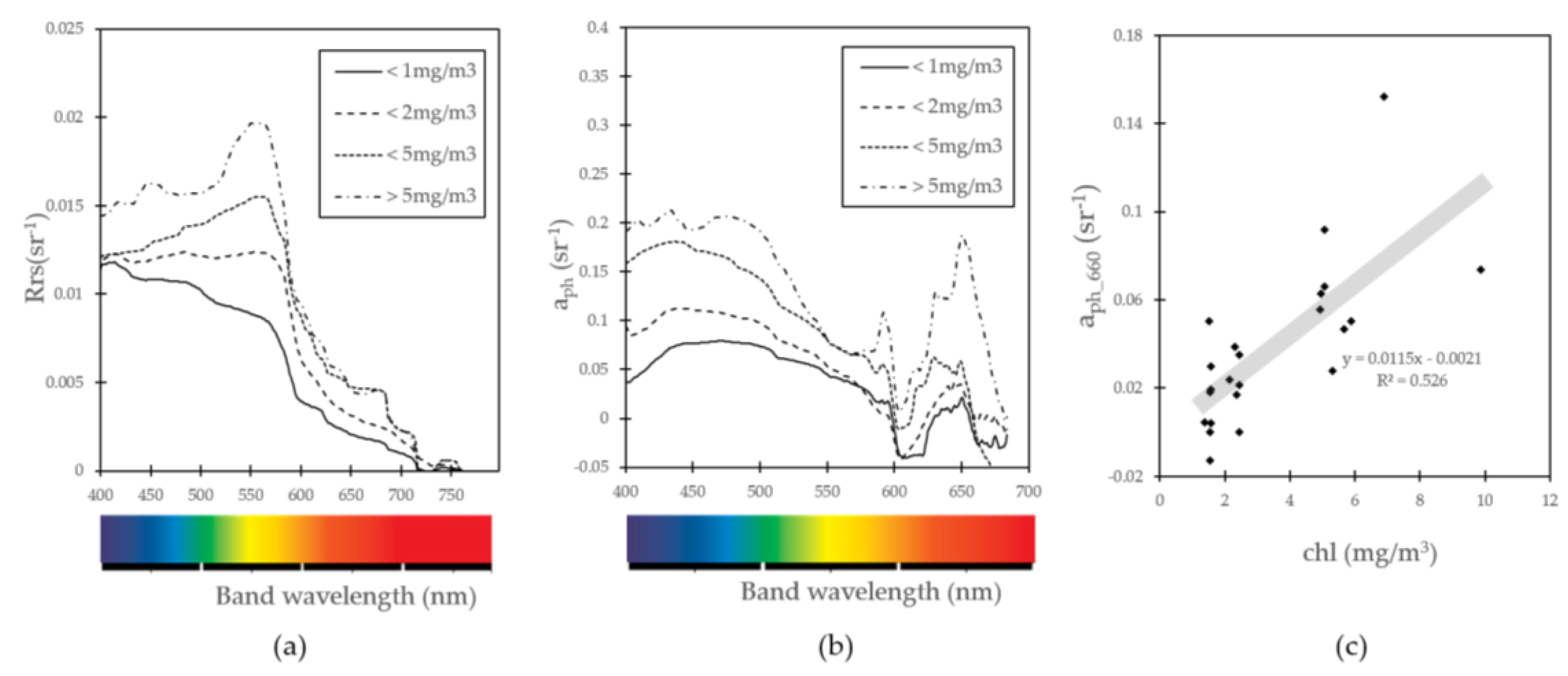
2.5. Phytoplankton Absorption Coefficent Spectrum

We applied bio-optical models to determine phytoplankton absorption coefficients from water leaving reflectance. There are two commonly used approaches in bio-optics, QAA [20] and GSM01 [19]. GSM01 retrieves simultaneous estimates for chlorophyll-a concentration, the absorption coefficients for dissolved, and detrital materials and particulate backscatter. Model parameters are then tuned through simulated annealing. The GSM01 model decreases residual errors from satellite and estimated Rrs through a multiple iteration approach (Maritorena, et al. [19]). The QAA (Lee, et al. [19]) analytically calculates coefficient values of total absorption and backscattering from remote sensing reflectance. In comparison to GSM01, the QAA approach has the benefit of not requiring any prior information about the spectral shape of a_Φ(λ) and thereby reduces potential errors and uncertainties with spectral models or inappropriate spectral shapes [19].

Considering the uniqueness of SO water optics [13,14], we intended to keep more original Rrs signals in phytoplankton absorption coefficients. Therefore, we applied QAA approach to invert the in situ Rrs and expanded the single band absorption into whole visible bands by introducing some of GSM01 equations. The QAA approach we applied here followed its V5 coefficients [30] and pure water absorption [31]. Details are shown in Appendix A.

Ciotti et al. [32] developed a micro-pico cell-size composition estimation approach from absorption coefficient spectrum. They used least-square fitting to gain abundance ($S_{\langle f\rangle }$) of micro and pico cells using whole bands.

$$\widehat{a_{\langle ph\rangle }}\left(\lambda \right)=\left[S_{\langle f\rangle }\cdot \overline{a_{\langle pico\rangle }}\left(\lambda \right)\right]+\left[(1-S_{\langle f\rangle })\cdot \overline{a_{\langle micro\rangle }}\left(\lambda \right)\right]$$

(5)

where $\widehat{a_{\langle ph\rangle }}\left(\lambda \right)$ are phytoplankton absorption coefficients, $S_{\langle f\rangle }$ is abundance of pico-phytoplankton, $\overline{a_{\langle pico\rangle }}\left(\lambda \right)$ and $\overline{a_{\langle micro\rangle }}\left(\lambda \right)$ are standard pico- and micro-absorption coefficients per unit from Table 3 in Ciotti, et al. [32]. This algorithm was used to estimate micro-phytoplankton fractions.

3. Results

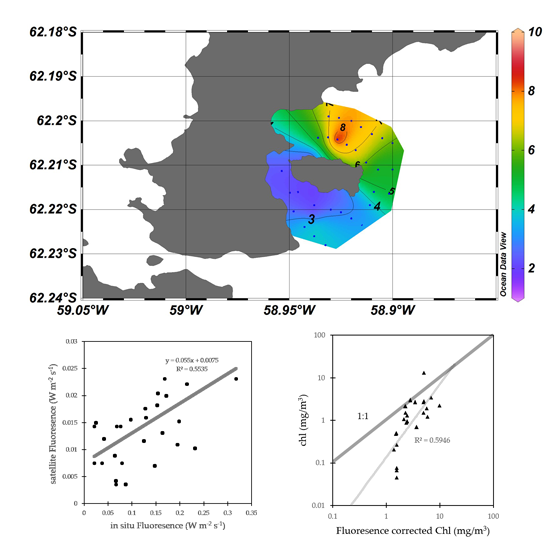
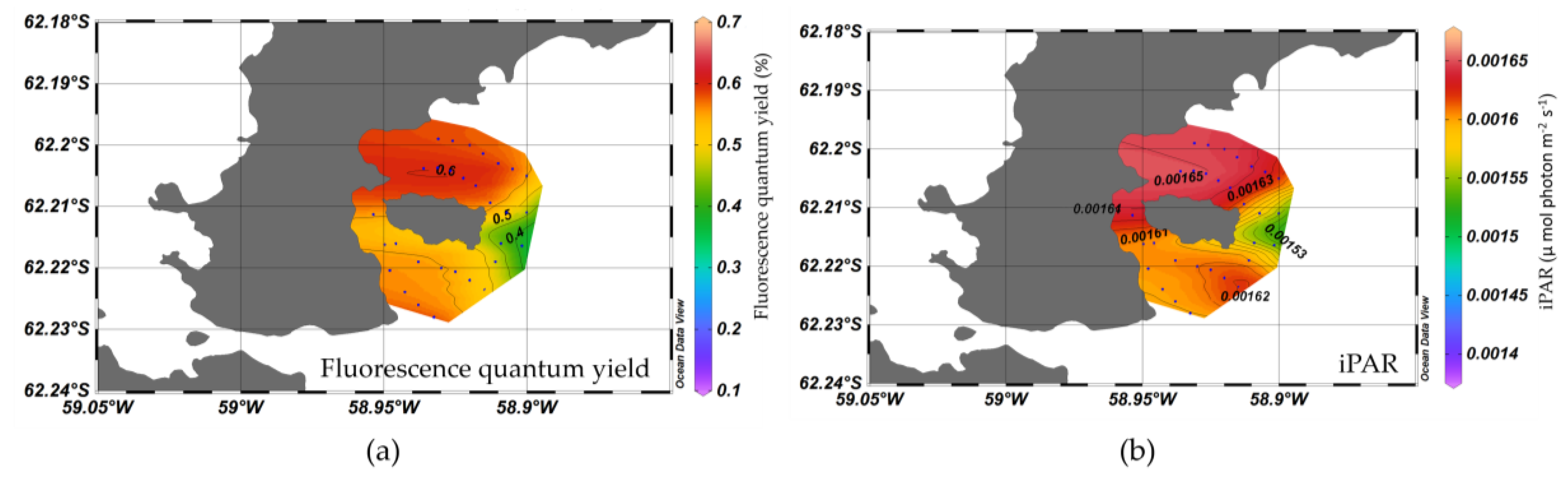
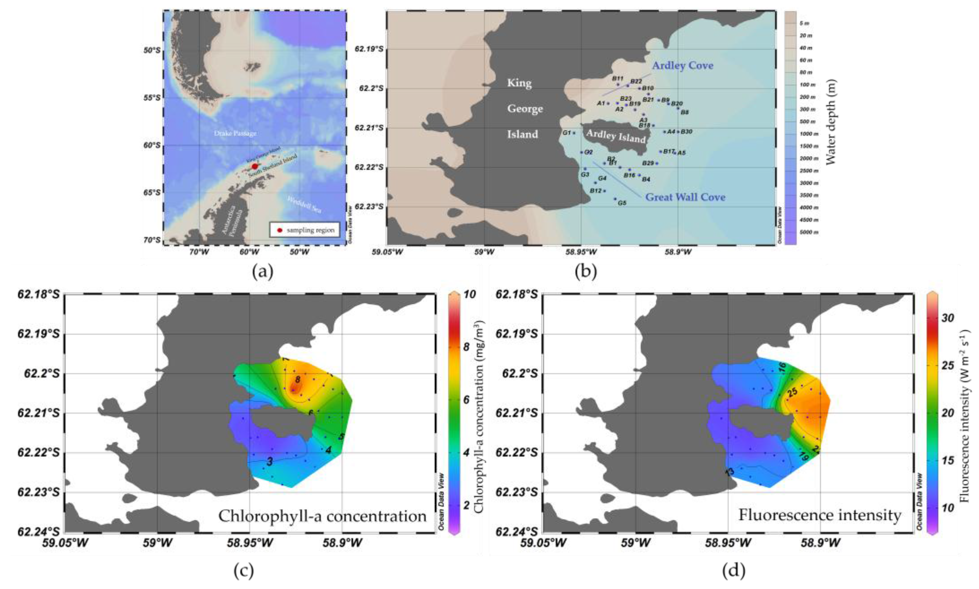
3.1. Spatial Distribution of Water Optical Properties

Chlorophyll-a varied significantly between Ardley Cove and Great Wall Cove (Figure 1c). Ardley Cove had a large phytoplankton bloom, with a maximum of chlorophyll-a at 9.87 mg/m³. Relatively low chlorophyll-a concentrations occurred in the Great Wall Cove, reaching only 1.37 mg/m³. Simultaneous in vivo fluorescence did not follow the same pattern, with the maximum occurring on the east side of Ardley Island instead of the north side (Figure 1d).

KGI Rrs spectrum produced 4 different shapes, with varied slopes between 550–560 nm (Figure 2a). These shapes were driven by chlorophyll-a concentration, with chlorophyll-a concentration increasing the overall Rrs value across all wavelengths less than 600 nm. For red bands higher than 600 nm, 4 Rrs spectra decreased significantly due to pure water absorption [32].

Despite the different Rrs spectral shapes for the various chlorophyll-a concentrations, the phytoplankton absorption coefficients showed similar curves after removing non-phytoplankton absorptions and particle backscattering coefficients (Figure 2b). Two obvious peaks appear in the blue and red bands of phytoplankton absorption spectra. Higher chlorophyll-a concentration has higher absorption coefficients, and the 660 nm absorption band has a good agreement with chlorophyll-a concentration (52.6%, p < 0.05) (Figure 2c).

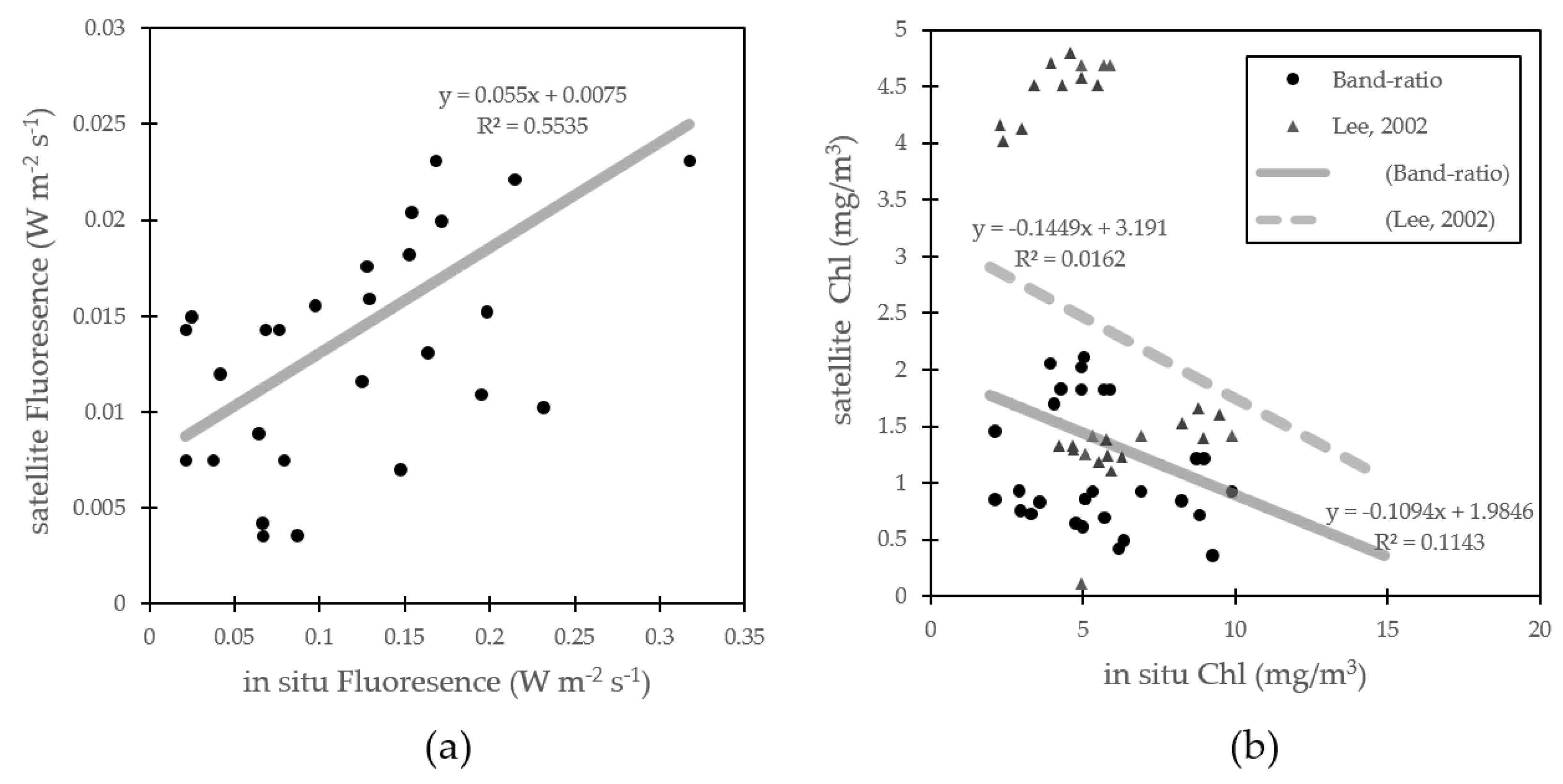
3.2. Algorithim Chlorophyll-a Estimation and In Situ/Satellite Match-Ups

Chlorophyll-a estimation from various algorithms were compared to in situ Rrs and residual errors were calculated. The results showed poor relationships with almost all previously developed algorithms (Table 1). All correlations were lower than 30%. An exception was the algorithm of Mitchell et.al [33]. Relative errors from estimated and in situ chlorophyll-a were greater than 60%. Although all these algorithms were built from the SO dataset, scarce samples in high latitude and high chlorophyll-a coastal water resulted in poor performance of chlorophyll-a estimation in KGI waters.

In addition, satellite-derived chlorophyll-a and fluorescence intensity from global empirical algorithms were evaluated. The comparison between in situ and satellite data showed a relatively good correlation with fluorescence intensity (55.35%) (Figure 3a). Direct band-ratio chlorophyll-a estimation showed a non-linear relationship with in situ chlorophyll-a with an 11.43% correlation (Figure 3b). Poor estimation was also apparent in the QAA bio-optical approach at a correlation of 1.62% (Figure 3b).

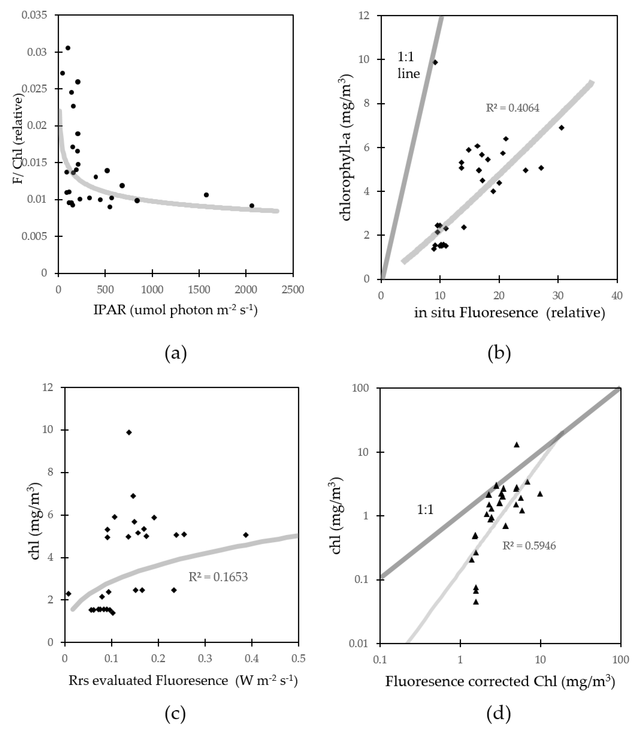
3.3. Fluorescence Approach Estimation for Chlorophyll-a

Based on the relatively good linear relationship between in situ and satellite fluorescence measurements, we explored the feasibility of using the fluorescence approach for estimating chlorophyll-a in KGI. This issue of non-linearity between in vivo fluorescence and chlorophyll-a, caused by NPQ under intense solar irradiance, was considered. Our measurements also showed a decreasing exponential phase of fluorescence per chlorophyll-a: iPAR (Figure 4a). Increasing solar irradiance decreases the fluorescence of chlorophyll-a yield, illustrating the impact of NPQ.

Previous research [23] reported a turning point of NPQ when iPAR reaches 100 μ mol/sec. After that point, NPQ will grow slowly. Since our measurements were collected in the southern summer with long daytime and high solar irradiance, the in vivo fluorescence influence on chlorophyll-a decreased (Figure 4a). Their correlation was 40.64%. High chlorophyll-a concentration samples had larger underestimation and deviation from 1:1 line than low chlorophyll-a concentration measurements (Figure 4b).

For the relationship between global empirical fluorescence from satellite and in situ chlorophyll-a (Figure 4c), the global coefficients do not work well in estimating chlorophyll-a in Ardley Cove since the fluorescence reacts a lot on phytoplankton physiology and iron stress [34]. Therefore, we optimized the three coefficients in the nFLH algorithm from the 30 in vivo fluorescence samples for the KGI region to produce the following algorithm:

$$\mathrm{nFLH}=\frac{13}{91}nl{w}_{678}+\frac{26}{91}nl{w}_{667}-\frac{53}{91}nl{w}_{748}, (r^2=65.15\%, \mathrm{rmse}=0.056)$$

(6)

where at 678, 667, and 748 nm, respectively. This optimization improved fluorescence estimation by about 10% from global empirical coefficients according to Figure 3a. Then, NPQ (FLH/iPAR) and phytoplankton absorption package correction (FLH/$\overline{a_{ph}}$, where $\overline{a_{ph}}$ is absorption mean between 300–700 nm per chlorophyll-a unit following Babin et al. [35]) were applied to the fluorescence estimation. The final fluorescence: chlorophyll-a relationship increased from original 40.64% to 59.46% (Figure 4d). Those two corrections referenced Behrenfeld et al. [23] correction in their Figure 2b,d. We do not introduce a global satellite average for iPAR and $a_{ph}$ to non-dimensionlization as they did in their correction. In our equation, the magnitude of in situ iPAR (10³) and $a_{ph}$ (10⁻³) balanced out and produced agreeable results.

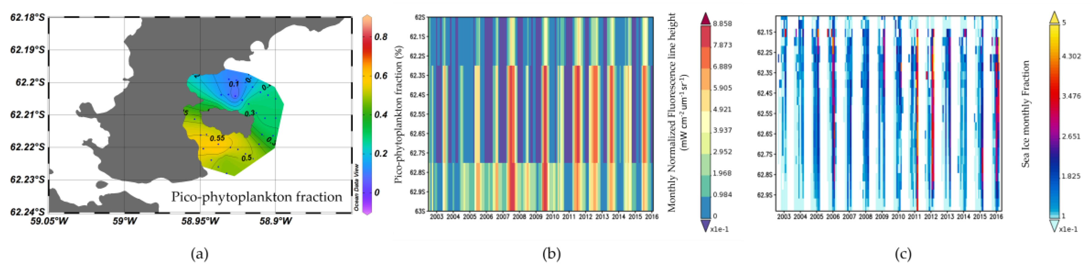
3.4. Nutrient, Light, and Phytoplankton Composition

Behrenfeld et al’s. [23] algorithm was useful in providing phytoplankton physiological status for our samples. According to Behrenfeld et al. [23], the remaining fluorescence signal divided by chlorophyll-a after NPQ and phytoplankton absorption package corrections are defined as fluorescence quantum yield and reflects the factors limiting phytoplankton growth (e.g., iron, light, or nitrogen/phosphorus). NPQ correction removes the photo-protection impacts on fluorescence intensity, and phytoplankton absorption package correction decreases the gaps between various phytoplankton communities. Fluorescence quantum yield is then quantified to global phytoplankton growth limitation factors where > 1.4% stands for iron limitation and < 1.4% means light, nitrogen/phosphorus limitation (in Figure 4 from their publication). The quantum yield in our samples was < 0.7% indicating that light and nitrogen/phosphorus limitation is greater in KGI Great Wall Cove than Ardley Cove (Figure 5a).

The spatial pattern of iPAR (Figure 5b) is similar to fluorescence quantum yield and chlorophyll-a in Figure 1c., which showed a stronger positive link between solar irradiance and phytoplankton biomass.

Phytoplankton size, deduced from the phytoplankton absorption coefficients, showed that the dominant phytoplankton in the bloom area are micro-size algae (> 20μm) (Figure 6a). The abundance of micro-size algae occupied 79.58% of the entire bloom phytoplankton community in Ardley Cove during our study. The mean residual error for Sf (pico-phytoplankton fraction estimation) is 16.54%.

Additionally, satellite-estimated chlorophyll-a and sea ice in this area show an increasing trend after 2002 (Figure 6b,c). When we focus on the year with extended sea ice coverage and high sea ice concentration (2009, 2011, and 2015), fluorescence intensity also increased in the following southern summer (2010, 2012, and 2016). Those years with high phytoplankton concentrations included 2010 [7]. It is noted that the fluorescence data shown here did not go through NPQ and phytoplankton absorption package corrections, so Figure 6b illustrates the relative trend with in the most recent decade.

4. Discussion

4.1. Fluorescence Approach Estimation for Chlorophyll-a

Light energy is an important factor regulating phytoplankton growth in KGI though photo-inhibition. The spatial pattern of IPAR (Figure 5b), which showed good agreement with chlorophyll-a concentration (Figure 1c), clearly illustrated the influence of light limitation on phytoplankton growth. This physical condition prevents optimal light for phytoplankton growth and this along with intense wind and terrigenous particles, typically leads to low primary productivity KGI [25]. From the perspective of this study, low light conditions ensured the reliability of the fluorescence approach and the nFLH algorithm.

Studies have shown improved application of the baseline fluorescence approach in case II waters over the global blue-green band-ratio algorithms [36]. The fluorescence approach also has higher effectiveness than the semi empirical algorithms like QAA (this study). Studies have also shown that inefficiencies in the SO bio-optics algorithms is generated from green band reflectance, leading to an obvious underestimation in chlorophyll-a when using global empirical coefficients [9]. In addition, the blue band is highly affected by CDOM, whose absorption coefficient was reported to occupy 70% of the non-water components in WAP (west of the Antarctica Peninsula) [37]. The absorption spectrum of CDOM has decreasing exponential influence, showing less influence on longer bands. Since the red band has longer wavelengths in the visible band, the selection of red bands will introduce less contamination in CDOM rich waters.

Conversely, this band selection has some issues. The red/NIR bands are more susceptible to atmospheric interference. Two recent programs, SOCTRATES [16] and WCRP [38] focused on the SO atmosphere, intend to improve the understanding of clouds, aerosols, air-sea exchanges over the SO. The improvement of SO atmospheric model will further meet the demands of input parameters for ocean color estimation in the near future.

SST-based corrections of fluorescence intensity have also been applied to SO waters. Browning et al. [39] found that extremely low SST in the SO has a strong connection with NPQ parameters and can be used to correct field chlorophyll-a fluorescence signals. They showed highly variable phytoplankton physiology features and communities under regional irradiance conditions and suggested more regional studies on NPQ capacity impacts. However, this correction needs an empirical relationship between SST and physiology coefficient B and was not applied in this study.

The byproduct of fluorescence quantum yield from the fluorescence approach also has a significant role in estimating primary productivity. State-of-the-art algorithms for primary productivity estimation are mainly based on chlorophyll-a absorption-fluorescence quantum yield equation or a photosynthesis-irradiance equation [40]. If we improve the estimation of fluorescence quantum yield from space, we will improve estimation for SO phytoplankton photosynthesis and carbon export. This will lead to a clearer understanding of the role of the SO in global climate change.

4.2. Factors on Phytoplankton Bloom in KGI

As an island hosting several international research stations, the ecological trend of the coastal waters surrounding KGI deserves attention. Historical records in KGI have shown that no phytoplankton blooms [6] occurred in these waters until 2010, during which maximum chlorophyll-a reached 20 mg/m³. Research has assumed that the increasing phytoplankton growth was exacerbated by global warming [25]. This manuscript documented another phytoplankton bloom in 2016 and attempted to determine its potential cause from optics and satellite history records. Iron limitation was widely observed in SO phytoplankton growth, which leads to ferredoxin deficiency in photosystem I and decreases photosynthetic efficiency. Iron depletion is reported as a major restriction for SO primary productivity [41,42]. However, previous research in KGI found no obvious nutrient or iron deficiencies in phytoplankton growth [43]. The microphytoplankton dominant features in this bloom (Figure 6a) further confirms iron enrichment because micro-size cells favor the iron abundant water. Micro-phytoplankton maintains a high growth rate in iron rich water, and their large size prevents zooplankton grazing [44].

Diatoms found around the WAP are larger in size than those found in other regions [44,45]. The phytoplankton bloom reported in 2010 was dominated by micro-algae (e.g., Porosira glacialis, Thalassiosira antarctica, and T. ritscheri [25]). Phytoplankton tends to adapt their cellular physiology to optimize light harvesting and photoreception [44]. Generally, small size algae benefit from light limited conditions due to their high absorption-photosynthesis effectiveness and small cellular shading [46]. Micro-size algae have more self-protection under high light conditions because their large surface area will cause low absorption-photosynthesis effectiveness. Therefore, for the micro-phytoplankton dominant bloom in KGI, nutrient support and zooplankton grazing has more influence on phytoplankton community composition than light limitation.

Owing to extended sea ice coverage and high sea ice concentration (Figure 6b,c), KGI has more fresh water input following southern summer to form strong stratification and keep phytoplankton in surface waters. This shallow mixed layer increases the probability for phytoplankton to absorb light energy. In addition, sea ice melt brings nutrients for algal growth [46,47,48,49]. The increasing trend of sea ice increases nutrients input (e.g., iron or micronutrients), which will lead to phytoplankton blooms in spring and summer. In addition, phytoplankton tends to bloom in marginal sea ice regions in the coastal ocean of the SO [46,47,48,49]. Therefore, increasing sea ice extent and coverage in KGI is a likely trigger for increased phytoplankton blooms.

4.3. Errors for Fluorescence Approach Estimating Chlorophyll-a

Two factors are responsible for accurate satellite estimation of chlorophyll-a. These include the sea-air model for calculating chlorophyll-a from water leaving Rrs and the atmospheric radiation transfer model to transfer top-of-atmosphere radiance into water leaving Rrs. Atmospheric correction has a large probability of introducing errors, because its signal occupies 90% of the total signal received at the satellite [50]. Therefore, atmospheric correction deserves great attention, particularly in improving its accuracy. Until now, there has not been a proper high latitude atmospheric correction model for the southern hemisphere and high cloud coverage in the SO creates a challenge for accurate atmospheric correction [16,17,51,52,53].

Atmospheric correction requires several steps to remove the influence of the atmosphere, such as single scattering, multiple molecular scattering, aerosol/ozone, and other gas absorption [54]. The procedure usually removes cloud contaminated pixels by the threshold of the near infrared band albedo. However, this method does not work well on cloud edges. Current satellite algorithms provide estimates of cloud optical thickness [55], which can be used to quantify the impacts of clouds on ocean color data in the near future.

The ocean color signal reflected from water is generally the integrated light reflected from the light penetration depth [56,57]. With increasing depth, deep waters have less contribution to the water modulated reflectance signals. However, we still cannot ignore it in chlorophyll-a inversion algorithms. In the SO, the deep chlorophyll-a maximum increases the contribution from deeper waters. Research seldom applies chlorophyll-a profiles and integrated chlorophyll-a signals to compare in situ and satellite match-ups. Current reports have already shown the obvious underestimation from satellite algorithms [6,7,8,9,10,11]. If considering the deep chlorophyll-a maximum and chlorophyll-a profile, there is a larger underestimation in SO chlorophyll-a retrieval. Chlorophyll-a profile estimation should be considered in future research. In fact, due to wind mixing, a deep chlorophyll-a maximum is a common situation in the SO [58,59]. Sullivan et al. [60] built a model on polar phytoplankton growth and reduction. They found that there is a high probability of maintaining a subsurface chlorophyll-a maximum during the post-bloom period.

5. Conclusions

Decades of development in satellite ocean color has produced multiple algorithms to detect, among other things, chlorophyll-a, fluorescence intensity, particulate organic carbon, photosynthetic available radiation. Satellites provide almost every parameter needed for observation and understanding the global ocean. However, the uncertainty of those parameters varies between regions. Our research validated the fluorescence approach to estimate chlorophyll-a concentration in KGI, resulting in a good agreement (59.46%) at this high latitude, high chlorophyll-a region. The phytoplankton bloom in 2016 showed that the dominant phytoplankton is micro-phytoplankton, occupying 79.58% of the total phytoplankton community in Ardley Cove. Increasing sea ice coverage and sea ice concentration are possible reasons for the increasing occurrence phytoplankton blooms in the recent decade. Due to NPQ, the fluorescence approach does not accurately estimate chlorophyll-a in places that have intense solar irradiance. However, the fluorescence approach and red band selection has notable advantages in avoiding CDOM interference from blue bands and decreasing gaps from the peculiar bio-optics of SO green bands. Our future work intends to validate and extend the application of this algorithm to the entire SO. The photosynthesis mechanism revealed by the fluorescence approach will provide more information on SO primary productivity estimation and its role on global carbon cycling.

References

1. Falkowski, P.G. The power of plankton. Nature 2012. [Google Scholar] [CrossRef] [PubMed]
2. Pope, A.; Wagner, P.; Johnson, R.; Baeseman, J.; Newman, L. Community review of Southern Ocean satellite data needs. Antarct. Sci. 2016. [Google Scholar] [CrossRef]
3. Babin, M.; Arrigo, K.; Bélanger, S.; Forge, M.-H. Ocean Colour Remote Sensing in Polar Seas; IOCCG Report Series, No. 16; International Ocean Colour Coordinating Group: Dartmouth, NS, Canada, 2015. [Google Scholar]
4. Reynolds, R.A.; Stramski, D.; Mitchell, B.G. A chlorophyll-a-dependent semi-analytical reflectance model derived from field measurements of absorption and backscattering coefficients within the Southern Ocean. J. Geophys. Res. 2001, 106, 7125–7138. [Google Scholar] [CrossRef]
5. Marrari, M.; Hu, C.; Daly, K. Validation of SeaWiFS chlorophyll-a a concentrations in the Southern Ocean: A revisit. Remote Sens. Environ. 2006, 105, 367–375. [Google Scholar] [CrossRef]
6. Moore, J.K.; Abbott, M.R. Phytoplankton chlorophyll-a distributions and primary production in the Southern Ocean. J. Geophys. Res. Ocean. 2000, 105, 28709–28722. [Google Scholar] [CrossRef]
7. Dierssen, H.M.; Smith, R.C. Bio-optical properties and remote sensing ocean color algorithms for Antarctic Peninsula waters. J. Geophys. Res. 2000, 105, 26301–26312. [Google Scholar] [CrossRef]
8. Gregg, W.W.; Casey, N.W. Global and regional evaluation of the SeaWiFS chlorophyll-a data set. Remote Sens. Environ. 2004, 93, 463–479. [Google Scholar] [CrossRef]
9. Kwok, R.; Comiso, J.C. Spatial patterns of variability in Antarctic surface temperature: Connections to the southern hemisphere annular mode and the southern oscillation. Geophys. Res. Lett. 2002. [Google Scholar] [CrossRef]
10. Gabric, A.J.; Shephard, J.M.; Knight, J.M.; Jones, G.; Trevena, A.J. Correlations between the satellite-derived seasonal cycles of phytoplankton biomass and aerosol optical depth in the Southern Ocean: Evidence for the influence of sea ice. Global Biogeochem. Cycles. 2005, 19, 1–10. [Google Scholar] [CrossRef]
11. Friedrichs, M.A.; Carr, M.E.; Barber, R.T.; Scardi, M.; Antoine, D.; Armstrong, R.A.; Asanuma, I.; Behrenfeld, M.J.; Buitenhuis, E.T.; Chai, F.; et al. Assessing the uncertainties of model estimates of primary productivity in the tropical Pacific Ocean. J. Mar. Syst. 2009, 76, 113–133. [Google Scholar] [CrossRef]
12. Zeng, C.; Xu, H.; Fischer, A. M. Chlorophyll-a estimation around the Antarctica peninsula using satellite algorithms: hints from field water leaving reflectance. Sensors 2016. [Google Scholar] [CrossRef] [PubMed]
13. Szeto, M.; Werdell, P.J.; Moore, T.S.; Campbell, J.W. Are the world’s oceans optically different? J. Geophys Res. 2011. [Google Scholar] [CrossRef]
14. Arrigo, K.R.; van Dijken, G.L.; Bushinsky, S. Primary production in the Southern Ocean, 1997–2006. J. Geophys. Res. 2008. [Google Scholar] [CrossRef]
15. Bélanger, S.; Ehn, J.K.; Babin, M. Impact of sea ice on the retrieval of water-leaving reflectance, chlorophyll-a a concentration and inherent optical properties from satellite ocean color data. Remote Sens. Environ. 2007, 111, 51–68. [Google Scholar] [CrossRef]
16. Wang, M.; Shi, W. Detection of ice and mixed ice–water pixels for MODIS ocean color data processing. IEEE Trans. Geosci. Remote Sens. 2009, 47, 2510–2518. [Google Scholar] [CrossRef]
17. McFarquhar, G.M.; Wood, R.; Bretherton, C.S.; Alexander, S.; Jakob, C.; Marchand, R.; Protat, A.; Quinn, P.; Siems, S.T.; Weller, R.A. The southern ocean clouds, radiation, aerosol transport experimental study (SOCRATES): An observational campaign for determining role of clouds, aerosolsand radiation in climate system. In Proceedings of the 2014 AGU Fall Meeting, San Francisco, CA, USA, 15–19 December 2014.
18. Kay, J.E.; Medeiros, B.; Hwang, Y.T.; Gettelman, A.; Perket, J.; Flanner, M.G. Processes controlling Southern Ocean shortwave climate feedbacks in CESM. Geophys. Res. Lett. 2014, 41, 616–622. [Google Scholar] [CrossRef]
19. Maritorena, S.; Siegel, D.A.; Peterson, A. Optimization of a semi-analytical ocean color model for global scale applications. Appl. Opt. 2002, 41, 2705–2714. [Google Scholar] [CrossRef] [PubMed]
20. Lee, Z.; Carder, K.L.; Arnone, R.A. Deriving inherent optical properties from water color: A multiband quasi-analytical algorithm for optically deep waters. Appl. Opt. 2002, 41, 5755–5772. [Google Scholar] [CrossRef] [PubMed]
21. Xing, X.; Claustre, H.; Blain, S.; D’Ortenzio, F.; Antoine, D.; Ras, J.; Guinet, C. Quenching correction for in vivo chlorophyll-a fluorescence acquired by autonomous platforms: A case study with instrumented elephant seals in the Kerguelen region (Southern Ocean). Limnol. Oceanogr. Method. 2012, 10, 483–495. [Google Scholar] [CrossRef]
22. Palmer, S.C.; Hunter, P.D.; Lankester, T.; Hubbard, S.; Spyrakos, E.; Tyler, A.N.; Presing, M.; Horvath, H.; Lamb, A.; Balzter, H.; et al. Validation of Envisat MERIS algorithms for chlorophyll-a retrieval in a large, turbid and optically-complex shallow lake. Remote Sens. Environ. 2015, 157, 158–169. [Google Scholar] [CrossRef] [Green Version]
23. Behrenfeld, M.J.; Westberry, T.K.; Boss, E.; O’Malley, R.T.; Siegel, D.A.; Wiggert, J.D.; Franz, B.A.; McClain, C.R.; Feldman, G.C.; Doney, S.C.; et al. Satellite-detected fluorescence reveals global physiology of ocean phytoplankton. Biogeosciences 2009, 6, 779–794. [Google Scholar] [CrossRef]
24. Schloss, I.R.; Abele, D.; Moreau, S.; Demers, S.; Bers, A.V.; González, O.; Ferreyra, G.A. Response of phytoplankton dynamics to 19-year (1991–2009) climate trends in Potter Cove (Antarctica). J. Marine Syst. 2012, 92, 53–66. [Google Scholar] [CrossRef]
25. Schloss, I.R.; Wasilowska, A.; Dumont, D.; Almandoz, G.O.; Hernando, M.P.; Michaud-Tremblay, C.A.; Saravia, L.; Rzepecki, M.; Monien, P.; Monien, D.; et al. On the phytoplankton bloom in coastal waters of southern King George Island (Antarctica) in January 2010: An exceptional feature? Limnol. Oceanogr. 2014. [Google Scholar] [CrossRef]
26. Mueller, J.L.; Fargion, G.S.; McClain, C.R.; Pegau, S.; Zanefeld, J.R.V.; Mitchell, B.G.; Kahru, M.; Wieland, J.; Stramska, M. Ocean Optics Protocols for Satellite Ocean Color Sensor Validation, Revision 4, Volume Iv: Radiometric Measurements and Data Analysis Protocols; Goddard Space Flight Space Center: Greenbelt, MD, USA, 2003. [Google Scholar]
27. Tang, J.W.; Tian, G.L.; Wang, X.Y.; Wang, X.M.; Song, Q.J. The methods of water spectra measurement and analysis i: Above-water method. J. Remote Sens. Beijing 2004, 8, 37–44. [Google Scholar]
28. Mobley, C. Overview of Optical Oceanography. Available online: http://www.oceanopticsbook.info/view/overview_of_optical_oceanography/reflectances (accessed on 25 June 2015).
29. Kohavi, R. A study of cross-validation and bootstrap for accuracy estimation and model selection. In Proceedings of the 14th International Joint Conference on Artificial Intelligence, Montreal, QB, Canada, 20–25 August 1995.
30. Lee, Z.P.; Lubac, B.; Werdell, J.; Arnone, R. An update of the Quasi-Analytical Algorithm (QAA_v5). Available online: http://www.ioccg.org/groups/Software_OCA/QAA_v5.pdf (accessed on 28 July 2009).
31. Pope, R.M.; Fry, E.S. Absorption spectrum (380–700 nm) of pure water. II. Integrating cavity measurements. Appl. Opt. 1997, 36, 8710–8723. [Google Scholar] [CrossRef] [PubMed]
32. Ciotti, Á.; Lewis, M.R.; Cullen, J.J. Assessment of the relationships between dominant cell size in natural phytoplankton communities and the spectral shape of the absorption coefficient. Limnol. Oceanogr. 2002, 2, 404–417. [Google Scholar] [CrossRef]
33. Mitchell, B.G.; Kahru, M. Bio-optical algorithms for ADEOS-2 GLI. J. Remote Sens. Soc. Jpn. 2009, 29, 80–85. [Google Scholar]
34. Behrenfeld, M. J.; Halsey, K.; Milligan, A. J. Evolved physiological responses of phytoplankton to their integrated growth environment. Phil. Trans. Royal Soc. B 2008, 363, 2687–2703. [Google Scholar] [CrossRef] [PubMed]
35. Babin, M.; Morel, A.; Gentili, B. Remote sensing of sea surface sun-induced chlorophyll-a fluorescence: consequences of natural variations in the optical characteristics of phytoplankton and the quantum yield of chlorophyll-a a fluorescence. Int. J. Remote Sens. 1996, 17, 2417–2448. [Google Scholar] [CrossRef]
36. Gower, J. On the use of satellite-measured chlorophyll fluorescence for monitoring coastal waters. Int. J. Remote Sens. 2016, 37, 2077–2086. [Google Scholar] [CrossRef]
37. Ortega-Retuerta, E.; Frazer, T.K.; Duarte, C.M.; Ruiz-Halpern, S.; Tovar-Sánchez, A.; Arrieta López de Uralde, J.M.; Reche, I. Biogeneration of chromophoric dissolved organic matter by bacteria and krill in the Southern Ocean. Limnol. Oceanogr. 2009, 54, 1941–1950. [Google Scholar] [CrossRef]
38. Bony, S.; Stevens, B.; Frierson, D.M.; Jakob, C.; Kageyama, M.; Pincus, R.; Shepherd, T.G.; Sherwood, S.C.; Siebesma, A.P.; Sobel, A.H.; et al. Clouds, circulation and climate sensitivity. Nat. Geosci. 2015, 8, 261–268. [Google Scholar] [CrossRef]
39. Browning, T.J.; Bouman, H.A.; Moore, C.M. Satellite-detected fluorescence: Decoupling nonphotochemical quenching from iron stress signals in the South Atlantic and Southern Ocean. Glob. Biogeochem. Cycles 2014, 28, 510–524. [Google Scholar] [CrossRef]
40. Sathyendranath, S.; Platt, T. Spectral effects in bio-optical control on the ocean system. Oceanologia. 2007, 49, 5–39. [Google Scholar]
41. Boyd, P.W.; Arrigo, K.R.; Strzepek, R.; Dijken, G.L. Mapping phytoplankton iron utilization: Insights into Southern Ocean supply mechanisms. J. Geophys. Res. Ocean. 2012, 117, 304–315. [Google Scholar] [CrossRef]
42. Boyd, P.W.; Watson, A.J.; Law, C.S.; Abraham, E.R.; Trull, T.; Murdoch, R.; Bakker, D.C.; Bowie, A.R.; Buesseler, K.O.; Chang, H.; et al. A mesoscale phytoplankton bloom in the polar Southern Ocean stimulated by iron fertilization. Nature 2000, 407, 695–702. [Google Scholar] [CrossRef] [PubMed]
43. Hewes, C.D.; Reiss, C.S.; Holm-Hansen, O. A quantitative analysis of sources for summertime phytoplankton variability over 18 years in the South Shetland Islands (Antarctica) region. Deep-Sea Res. Part I. Oceanogr. Res. Pap. 2009, 56, 1230–1241. [Google Scholar] [CrossRef]
44. Tripathy, S.C.; Pavithran, S.; Sabu, P.; Naik, R.K.; Noronha, S.B.; Bhaskar, P.V.; Anilkumar, N. Is phytoplankton productivity in the Indian Ocean sector of Southern? Curr. Sci. 2014, 107, 1019–1026. [Google Scholar]
45. Brody, E.; Mitchell, B.G.; Holm-Hansen, O.; Vernet, M. Species-dependent variations of the absorption coefficient in the Gerlache Strait. Antarct. J. USA 1992, 27, 160–162. [Google Scholar]
46. Finkel, Z.V.; Beardall, J.; Flynn, K.J.; Quigg, A.; Rees, T.A.V.; Raven, J.A. Phytoplankton in a changing world: cell size and elemental stoichiometry. J. Plankton Res. 2009, 32, 119–137. [Google Scholar] [CrossRef]
47. Smith, W.O.; Nelson, D.M. Phytoplankton bloom produced by a receding ice edge in the Ross Sea: Spatial coherence with the density field. Science 1985, 227, 163–166. [Google Scholar] [CrossRef] [PubMed]
48. Boetius, A.; Albrecht, S.; Bakker, K.; Bienhold, C.; Felden, J.; Fernández-Méndez, M.; Hendricks, S.; Katlein, C.; Lalande, C.; Krumpen, T.; et al. Export of algal biomass from the melting Arctic sea ice. Science 2013, 339, 1430–1432. [Google Scholar] [CrossRef] [PubMed]
49. Arrigo, K.R.; Lowry, K.E.; van Dijken, G.L. Annual changes in sea ice and phytoplankton in polynyas of the Amundsen Sea, Antarctica. Deep-Sea Res. Part II Top. Stud. Oceanogr. 2012, 71, 5–15. [Google Scholar] [CrossRef]
50. Gordon, H.R. Removal of atmospheric effects from the satellite imagery of the oceans. Appl. Opt. 1978, 17, 1631–1636. [Google Scholar] [CrossRef] [PubMed]
51. Behrangi, A.; Stephens, G.; Adler, R.F.; Huffman, G.J.; Lambrigtsen, B.; Lebsock, M. An update on the oceanic precipitation rate and its zonal distribution in light of advanced observations from space. J. Clim. 2014, 27, 3957–3965. [Google Scholar] [CrossRef]
52. Haynes, J.M.; L’Ecuyer, T.S.; Stephens, G.L.; Miller, S.D.; Mitrescu, C.; Wood, N.B.; Tanelli, S. Rainfall retrieval over the ocean with spaceborne W-band radar. J. Geophys. Res. 2009. [Google Scholar] [CrossRef]
53. Meskhidze, N.; Nenes, A. Phytoplankton and cloudiness in the Southern Ocean. Science 2006, 314, 1419–1423. [Google Scholar] [CrossRef] [PubMed]
54. Vermote, E.F.; Tanré, D.; Deuzé, J.L.; Herman, M.; Morcrette, J.J.; Kotchenova, S.Y. Second Simulation of A Satellite Signal in the Solar Spectrum-Vector (6SV), 6S User Guide Version 3. Available online: http://6s.ltdri.org/files/tutorial/6S_Manual_Part_1.pdf (accessed on 23 September 2016).
55. Marchand, R.; Ackerman, T.; Smyth, M.; Rossow, W.B. A review of cloud top height and optical depth histograms from MISR, ISCCP, and MODIS. J. Geophys. Res. 2010. [Google Scholar] [CrossRef]
56. Soppa, M.A.; Dinter, T.; Taylor, B.B.; Bracher, A. Satellite derived euphotic depth in the Southern Ocean: Implications for primary production modelling. Remote Sens. Environ. 2013, 137, 198–211. [Google Scholar] [CrossRef] [Green Version]
57. Lee, Z.; Weidemann, A.; Kindle, J.; Arnone, R.; Carder, K.L.; Davis, C. Euphotic zone depth: Its derivation and implication to ocean-color remote sensing. J. Geophys. Res. 2007. [Google Scholar] [CrossRef]
58. Schlitzer, R. Carbon export fluxes in the Southern Ocean: Results from inverse modeling and comparison with satellite-based estimates. Deep-Sea Res. Part II Top. Stud. Oceanogr. 2002, 49, 1623–1644. [Google Scholar] [CrossRef]
59. Uitz, J.; Claustre, H.; Griffiths, F.B.; Ras, J.; Garcia, N.; Sandroni, V. A phytoplankton class-specific primary production model applied to the Kerguelen Islands region (Southern Ocean). Deep-Sea Res. Part I. Oceanogr. Res. Pap. 2009, 56, 541–560. [Google Scholar] [CrossRef]
60. Sullivan, C.W.; McClain, C.R.; Comiso, J.C.; Smith, W.O. Phytoplankton standing crops within an Antarctic ice edge assessed by satellite remote sensing. J. Geophys. Res. Ocean. 1988, 93, 12487–12498. [Google Scholar] [CrossRef]
Figure 1. (a) Sampling area location. (b) Locations of in situ samples. (c) Chlorophyll-a spatial pattern interpolated from the in situ samples during January 2016. (d) In vivo fluorescence interpolated from the in situ samples during January 2016.
Remotesensing 09 00210 g001
Figure 2. (a) Four selected above water Rrs spectra. (b) Four featured phytoplankton absorption coefficients derived from Figure 2a using QAA v5 presented in Appendix A. (c) Correlation between phytoplankton absorption coefficients and in situ chlorophyll-a concentration.
Remotesensing 09 00210 g002
Figure 3. (a) Correlation between satellite derived fluorescence and in situ measured in vivo fluorescence (n = 28). The satellite fluorescence algorithm here is based on the global fluorescence coefficients from NASA ocean color group (https://oceancolor.gsfc.nasa.gov/atbd/nflh/). (b) Correlation between satellite and in situ chlorophyll-a concentrations. The satellite algorithm applied here is the OC3 global band-ratio (http://oceancolor.gsfc.nasa.gov/cms/atbd/chlor_a) and NASA IOP model derived absorption coefficient for phytoplankton (http://oceancolor.gsfc.nasa.gov/cms/atbd/giop).
Remotesensing 09 00210 g003
Figure 4. (a) Relationship between fluorescence per chlorophyll-a unit and iPAR. (b) Relationship between in situ chlorophyll-a and fluorescence intensity. (c) Relationship between in situ chlorophyll-a and in situ Rrs estimated fluorescence. (d) Relationship between in situ chlorophyll-a and in situ fluorescence estimated chlorophyll-a after regional coefficients improvement, NPQ correction and phytoplankton absorption package correction.
Remotesensing 09 00210 g004
Figure 5. (a) Fluorescence quantum yield interpolated from in situ samples during January 2016, and (b) iPAR spatial pattern interpolated from in situ samples during January 2016.
Remotesensing 09 00210 g005
Figure 6. (a) Pico-phytoplankton fraction spatial pattern retrieved from the in situ spectrum algorithm (Equation (5)) during January 2016 (b) Hovmoller longitude-average plots of satellite records on fluorescence estimated chlorophyll-a from Giovanni (http://giovanni.gsfc.nasa.gov/giovanni/). (c) Hovmoller longitude-average plots of satellite records on sea ice concentration from Giovanni.
Remotesensing 09 00210 g006