Article

Robinia pseudoacacia L. Flower Analyzed by Using An Unmanned Aerial Vehicle (UAV)

by
Christin Carl
1,2,*,
Dirk Landgraf
2,
Marieke Van der Maaten-Theunissen
3,
Peter Biber
1 and
Hans Pretzsch
1
1
Forest Growth and Yield Science, School of Life Sciences Weihenstephan, Technische Universität München, Hans-Carl-von-Carlowitz-Platz 2, 85354 Freising, Germany
2
Forestry and Ecosystem Management, University of Applied Science Erfurt, Leipziger Straße 77, 99085 Erfurt, Germany
3
Institute of Botany and Landscape Ecology, University of Greifswald, Soldmannstrasse 15, 17489 Greifswald, Germany
*
Author to whom correspondence should be addressed.
Remote Sens. 2017, 9(11), 1091; https://doi.org/10.3390/rs9111091
Submission received: 25 September 2017 / Revised: 21 October 2017 / Accepted: 24 October 2017 / Published: 26 October 2017
(This article belongs to the Section Forest Remote Sensing)

Abstract

:
Tree flowers are important for flower–insect relationships, seeds, fruits, and honey production. Flowers are difficult to analyze, particularly in complex ecosystems such as forests. However, unmanned aerial vehicles (UAVs) enable detailed analyses with high spatial resolution, and avoid destruction of sensitive ecosystems. In this study, we hypothesize that UAVs can be used to estimate the number of existing flowers, the quantity of nectar, and habitat potential for honeybees (Apis mellifera). To test this idea, in 2017 we combined UAV image analysis with manual counting and weighing of the flowers of eight-year-old black locust (Robinia pseudoacacia L.) trees to calculate the number of flowers, their surface area, and their volume. Estimates of flower surface area ranged from 2.97 to 0.03% as the flying altitude above the crowns increased from 2.6 m to 92.6 m. Second, for the horizontal analysis, a 133 m2 flower area at a one-hectare black locust plantation was monitored in 2017 by a UAV. Flower numbers ranged from 1913 to 15,559 per tree with an average surface area of 1.92 cm2 and average volume of 5.96 cm3. The UAV monitored 11% of the total surface and 3% of the total volume. Consequently, at the one-hectare black locust study area we estimate 5.3 million flowers (69 kg honey), which is sufficient for one bee hive to survive for one year.

1. Introduction

Flower production is essential for the survival of most plant species in the world, because it relates directly to the number of seeds produced. As a side effect, flowers provide ecosystem services, such as food for many insects via the flower-pollinator relationship. Moreover, humans have benefited for thousands of years; for example, by cultivating honeybees (Apis mellifera) for honey production or for the pollination of fruit trees. Furthermore, not only are tree flowers, but also the subsequent fruits and seeds, energy banks for many animals. However, detailed information about tree flowers, particularly those of black locust (Robinia pseudoacacia L.), is very limited.
Black locust is one of the most criticized non-native tree species in Germany and Europe [1] because its rootstocks spread into neighboring areas. Furthermore, black locust represses rare, native, and endangered species [2]. However, black locust also offers many advantages and thus may represent an opportunity for European forests in these times of climate change. For example, it is a fast growing, sun light loving, and unpretentious tree and can grow in poor-nutrient areas, such as former brown-coal mining areas. In addition, black locust starts flowering early, often at an age of six years [3] or younger. Many insects, especially Hymenoptera, such as A. mellifera, benefit from this service. Black locust honey is often sold as acacia honey [4], and in Hungary, the production of this type of honey is very common and economically important [3].
Many ecosystem structures and changes may be monitored via satellite data [5,6,7,8,9,10]. In forest ecosystems, the focus has been on the canopy structure [11,12,13], especially the leaf area index (LAI) [13,14,15,16,17], chlorophyll analysis [13,18,19], and discoloration caused by diseases or disturbance [20,21,22], particularly insects [23,24,25,26,27,28,29,30,31]. In Africa, flower cycles have been monitored by airplane remote sensing [32,33] as a guide for beekeepers. However, unmanned aerial vehicles (UAVs) allow monitoring with a much higher spatial resolution of small, specific, and detailed vegetation structures, such as flowers. In addition, UAVs combine quick turnaround times in combination with lower operational costs. Therefore, UAV data may provide an important supplement to data from satellites, airplanes, towers [34], and to field-collected data. In agriculture, the work done with information and communication technology is described as the fourth revolution. Smart farming is the key to developing sustainable agriculture, and UAVs are an important part of this strategy [35]. Scientific and practical examples of UAV use include the monitoring of agave crops [36], canola [37,38], maize [39,40], potato [41,42], wheat [42,43,44,45,46,47], sugarcane [48], viticulture [49,50], peach trees [51], olive trees [52,53,54], and papaya trees [55] in addition to the distribution of biological insecticides [56] and the control of drainage systems in agricultural areas [57]. UAVs are also a part of a new revolution in forestry management [58]. For example, UAVs are now used to find bark beetles as early as possible [59,60], to monitor the infestation levels of pests [61], to manage wild animals, develop forest inventories [58,62], monitor wind damage [63], schedule projects, exploit forests [64], and to quantify the expected seed production of beech trees [65]. In plant ecology, UAVs have been used for LAI analysis [66] and to analyze the structure of ultrafine dryland vegetation [67]. Furthermore, Mc Neil et al. [68] combined a UAV and ImageJ (a freeware Java-based image-processing program) to measure leaf-angle distribution in the canopies of broadleaved trees. MacInnis and Forrest [69] used ImageJ to quantify the pollen deposition of two Narcissus ssp. and strawberry (Fragaria x ananassa). Flower-health classification supported by digital-imaging techniques with ImageJ is the topic of Lino et al. [70].
In the present study, we use a UAV and flower analysis by ImageJ as an innovative and economical option to analyze the flowers of R. pseudoacacia and estimate the food base for Hymenoptera, especially A. mellifera. We investigate 13 different flying altitudes (Vertical Analysis), monitor a 50 × 50 m2 area (Horizontal Analysis), and seven sample trees (Flower Trees) in bloom in an eight-year-old black locust plantation. The flowers were counted, photographed, and weighed. Furthermore, we create two models: Model (1) solely base on the field-collected data, and Model (2), which combines the field-collected data with photographic data from the UAV.
The main idea of this study is to monitor the insect-biodiversity potential of black locust trees by indirect analysis. To demonstrate this method, we apply it to honeybees, although numerous opportunities exist for analyzing further insect species. Thus, this study represents a first step toward developing a method to analyze tree flowers, which may eventually evolve into an indirect method to analyze biodiversity. The research objectives of this study are (1) to adapt methods to classify flowers in black locust plantations via UAV red–green–blue (RGB) aerial imagery; and (2) to evaluate the number of flowers and the nectar production, and to assess the habitat for honeybees. The corresponding research questions are as follows:
Can UAVs be used to analyze flowers in R. pseudoacacia plantations?
(1)
What is the best flying altitude (FA) for the UAVs?
(2)
How much flower surface (2D) and volume (3D) can be detected by a UAV?
(3)
How many flowers are present per hectare, and per tree?
Is this method suitable to monitor the structure of the temporary habitat for honeybees?
(1)
What mass of nectar and honey (kg) can be produced by one hectare of eight-year-old R. pseudoacacia?
(2)
What population of honeybees can survive for one year from the flower production of a one-hectare black locust plantation?

2. Materials and Methods

2.1. Study Area

The study area is in northeastern Germany in the federal state of Brandenburg (13°50′57′′E, 51°32′20′′N, and 111 m above sea level). It has an annual precipitation of 555 mm and a mean annual temperature of 9.4 °C [71]. The study area was previously used for brown-coal mining and has now been recultivated with different tree species [72]. The black locust plantation under study was planted eight years ago. Blossoms flower at the end of May and at the beginning of June (29 May–2 June 2017). The analysis began with the flight of a hexacopter [56] on 29 May 2017.

2.2. Flower Analysis

The analysis was divided into three parts (Figure 1). First, a Vertical Analysis was done to determine differences in the detected study area and the best flying altitude. This was followed by a Horizontal Analysis to get an overview of the entire area. Finally, the Flower Trees were intensively analyzed to estimate the number of flowers and nectar for honeybees.

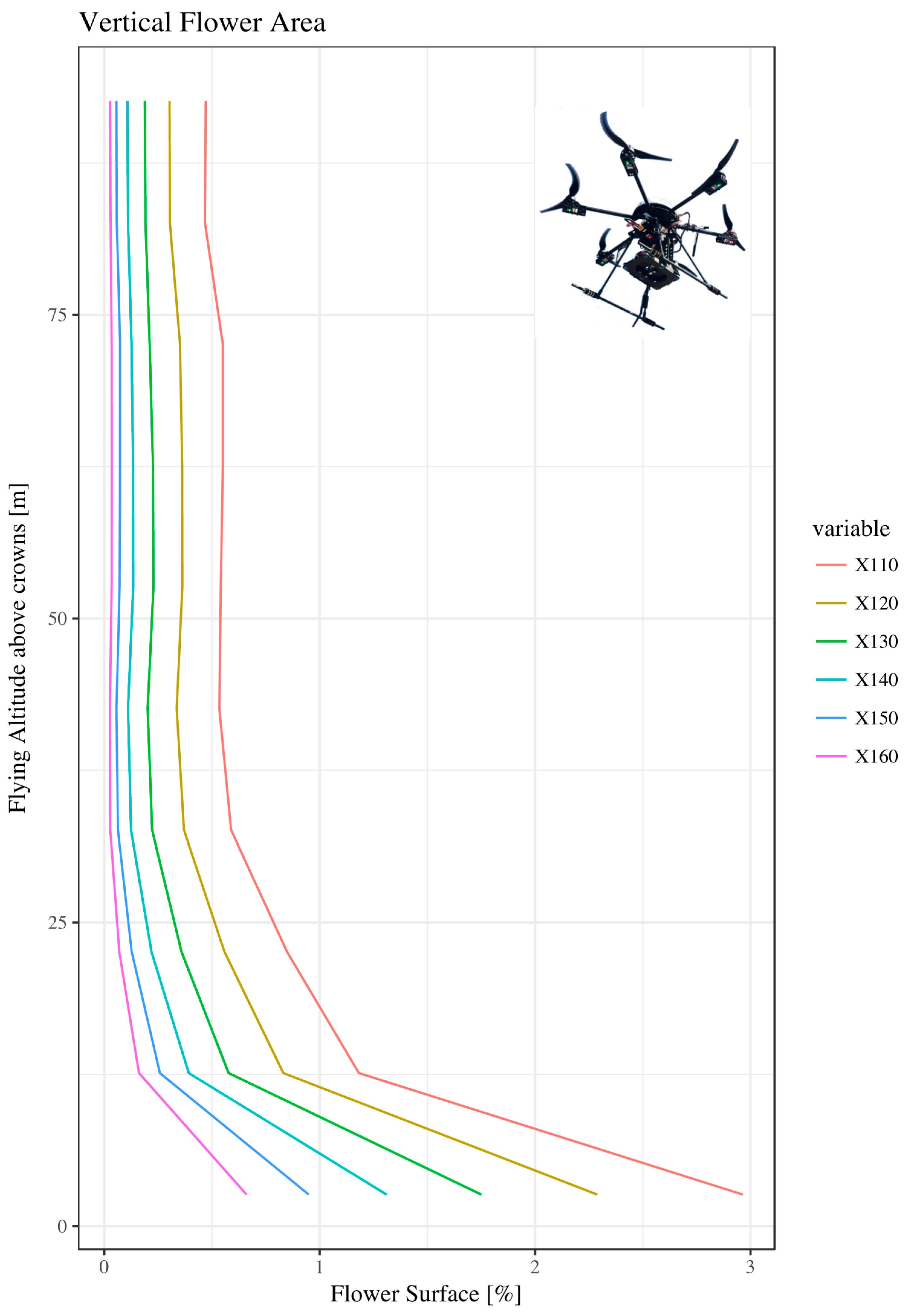
2.2.1. Vertical Analysis

For the Vertical Analysis we chose 13 different flying altitudes (FA) above the starting point: 20 to 50 m in 5 m steps, and 50 to 110 m in 10 m steps (Table 1). The FA above the starting point was determined by the UAV on-board computer. The FA above ground and above crown was calculated (Appendix A). A FA of 20 m above the starting point was chosen because it was the lowest FA the UAV could fly without significant buffeting of the canopy from rotor downwash. In total, 26 pictures were taken by the on-board MAPIR Survey2 RGB camera (MAPIR, San Diego, CA, USA) [74] for the Vertical Analysis.

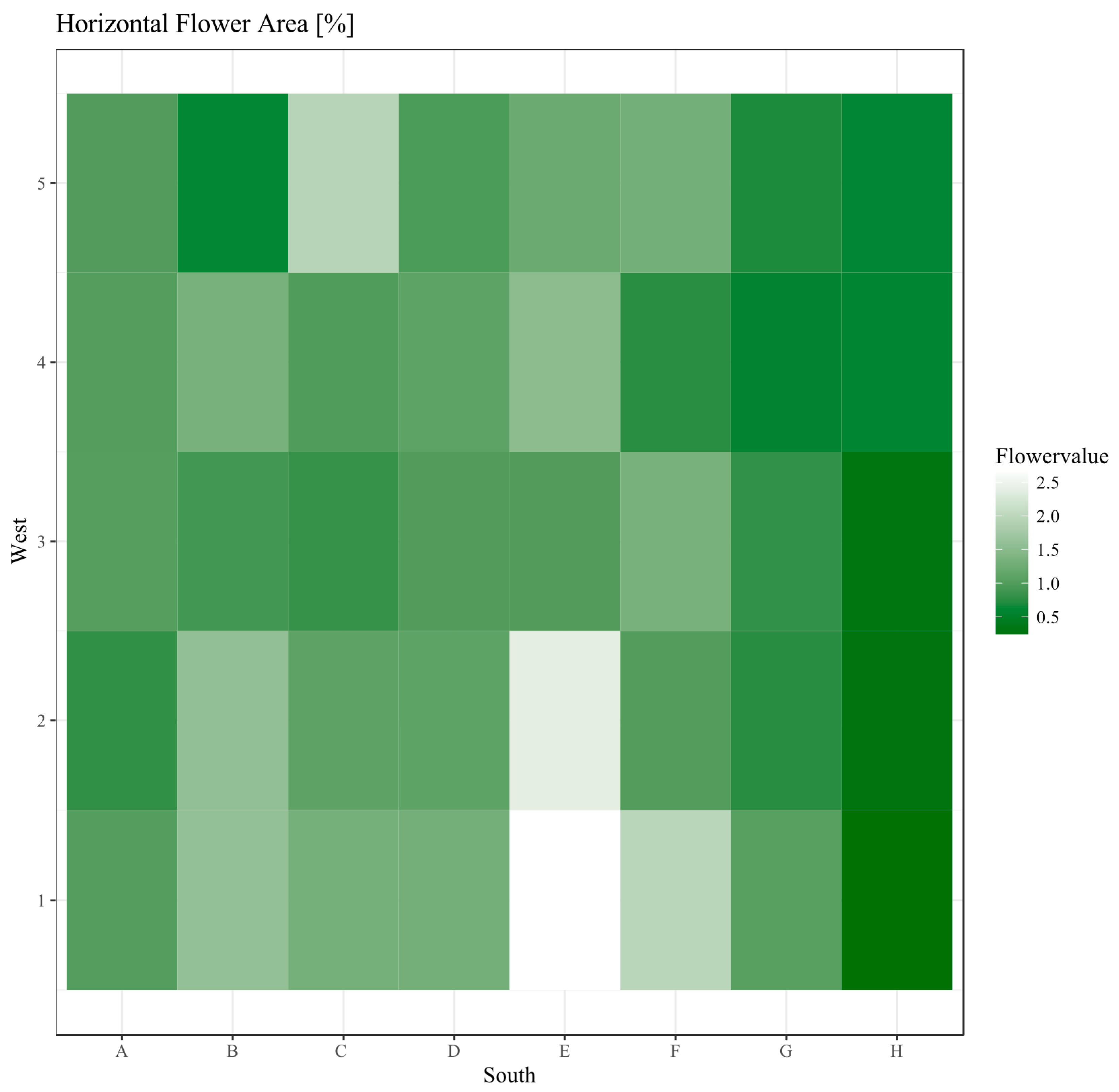
2.2.2. Horizontal Analysis

For the Horizontal Analysis, the hexacopter flew at a low FA (2.6–5.5 m above crowns, Table 2) above a 50 × 50 m2 square area. Therefore, 80 areas were delineated within a grid with a cell size of 6.2 m (8 x lines) by 5.0 m (10 y lines). Scale bars were positioned on the ground. The black border of each scale bar is 50 × 50 cm2 and the white panel is 25 × 25 cm2 (Figure 2). The Field of View (FOV) is based on sensor size (6.17472 mm × 4.63104 mm), focal distance (3.97 mm), and height above ground (m) (Table 2). The Ground Sample Distance (GSD) is calculated from the FOV and pixel values (4608 × 3456). Images are individually cropped to prevent the photographs from overlapping. All in all, 160 photographs (two photographs of each subarea) were created with a MAPIR Survey2 RGB camera (MAPIR, San Diego, CA, USA) [74] for the Horizontal Analysis. The FA is influenced by the slope of the area (Appendix A), and in each line the flying altitude above the starting point, ground, and crown varies (Table 2).

2.2.3. Flower Trees (UAV and Field Data Collection)

Seven Flower Trees were used to compare and supplement the UAV data with field-collected data. The scale bars were installed in the crowns of the Flower Trees, and the UAV flew to each Flower Tree separately. The flower area of each Flower Tree individually was calculated by using ImageJ (Section 2.2.4). The reference data consists of the manually analyzed flowers per tree. The Flower Trees are the base to estimate the relationship between flowers detected by UAV and the total number of manually counted flowers, the total flower surface, and the total flower volume. This relationship is used to calculate the number of flowers for the analyzed 50 × 50 m2 area and per hectare. For the field data collection, the seven marked Flower Trees were harvested shortly after the UAV flights (30 May–2 June 2017). Furthermore, each racemose inflorescence of each branch was analyzed, and the total number of flowers was counted. Next, 50 inflorescences were selected at random and the exact surface area of each flower was determined for 10 flowers from each inflorescence (500 flowers total). This was done by photographing each flower and using ImageJ [75,76] to determine the surface area. The binary function of ImageJ is helpful for measuring the surface area per flower. To calculate the flower volume (i.e., the 3-dimension flower surface (3D)), the flowers were weighed (digital precision scale ± 0.001 g, maximum 20 g). Therefore, we determine the total mass of each flower and the mass of a 1.0 cm2 area of each flower.
The relationship between the number of flowers and the percent of flower surface detected by the UAV is determined via a linear regression analysis and the coefficient of determination.

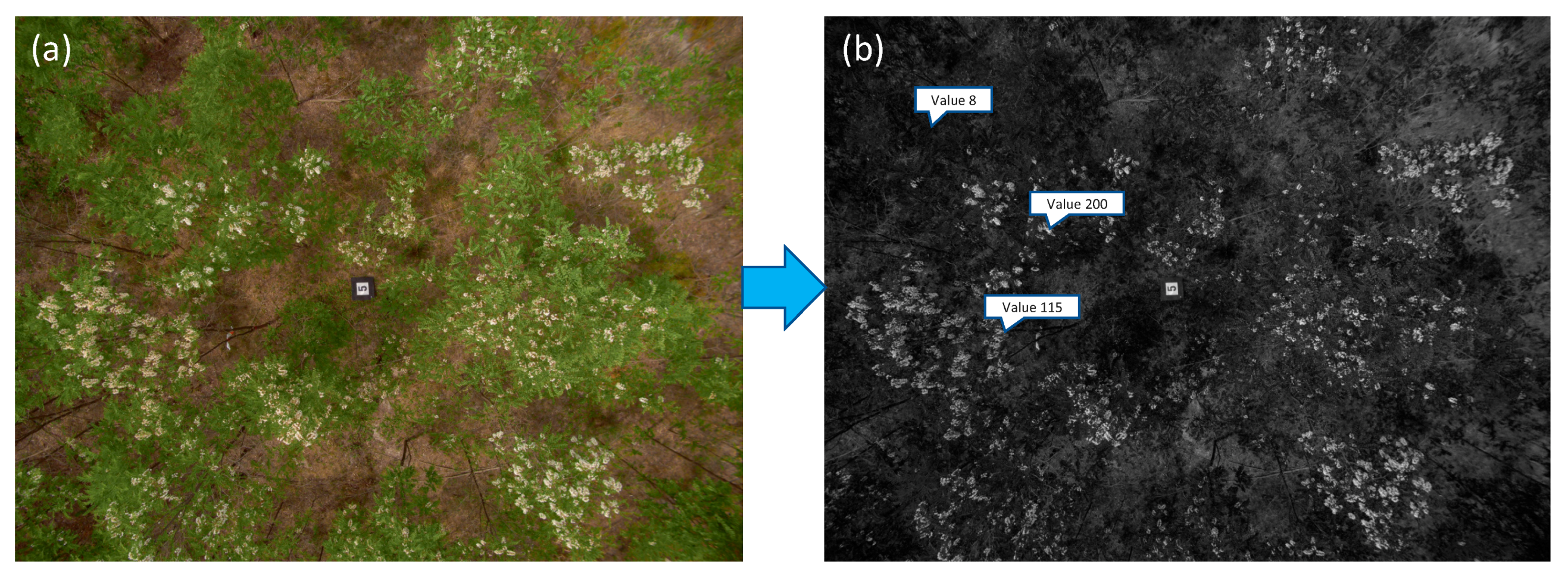
2.2.4. Image Analysis

ImageJ is used for image analysis. ImageJ is a free, Java-based image-processing program and Fiji is an open-source image-processing package that operates in the ImageJ software environment [75,76]. After converting the image to red, green, and blue channel, we used the blue channel for flower analyses. The advantage of the blue channel is that the tree biomass (leaves, weeds, branches) reflect poorly in the blue band. Therefore, a distinct boundary appears between flowers and tree (and weed) biomass (Figure 2).
The flower area was calculated after defining the threshold value for all three subdivisions: Vertical (threshold 110–160), Horizontal (threshold 140), and Flower Tree Analysis (threshold 140). By analyzing 12,500 pixels (ImageJ segmentation versus user/visual inspection of flowers), threshold 140 had the best Overall Accuracy (99.5%) and Kappa Coefficient (0.913) (Appendix A, Table A1). Threshold 120–150 had an almost perfect (0.81–1.0) level of agreement to the reference and threshold 110 and 160 were classified as substantial (0.61–0.81) by using the Kappa Coefficient [77,78]. Thresholds smaller than 140 had a low Users Accuracy for the Flower classification (Commission Error). Therefore, parts of the biomass and soil are classified as flowers. Increasing thresholds (>140) have a decreasing Producers Accuracy for the Flower classification (Omission Error). Consequently, flowers are classified as biomass. Hence, threshold 140 was used for Horizontal Analysis and the Flower Trees. The topology of the study area is rough; the angle of slope averaged 12°. Therefore, the FA at the starting point differs from the FA above the ground and crowns over the entire area (Vertical Analyses, Table 3), above Flower Trees, and in the Horizontal Analyses in each line (Figure 2, Table 2). Details of the computed FAs, scale bars, and the crown-correction factor appear in Appendix A, especially Figure A1 and Equations (A1)–(A7).

2.2.5. Models: Calculating Flower Number

We developed two models to calculate the number of flowers. First, by using only field-collected data, we calculate the flower number n flowers ( 1 ) by multiplying the average flower number n ¯ flowers of the Flower Trees and the counted number n trees of trees per hectare. Explicitly, Model (1) is calculated as follows:
n flowers ( 1 ) = n ¯ flowers n trees
In the second model, the flower number n flowers ( 2 ) is calculated based on the field-collected data combined with the UAV data. The flower area of one hectare (FoA) is determined by using the average percent yielded by the horizontal analysis of ¼ hectare and the average flower surface area FSU detected by the UAV. Explicitly, Model (2) is calculated as follows:
n flowers ( 2 ) = F o A F S U
All analyses were done by using R, version R 3.3.2 [79], with the R packages “stats” [79], “ape” [80], “ggplot2” [81], “png” [82], and “gridGraphics” [83].

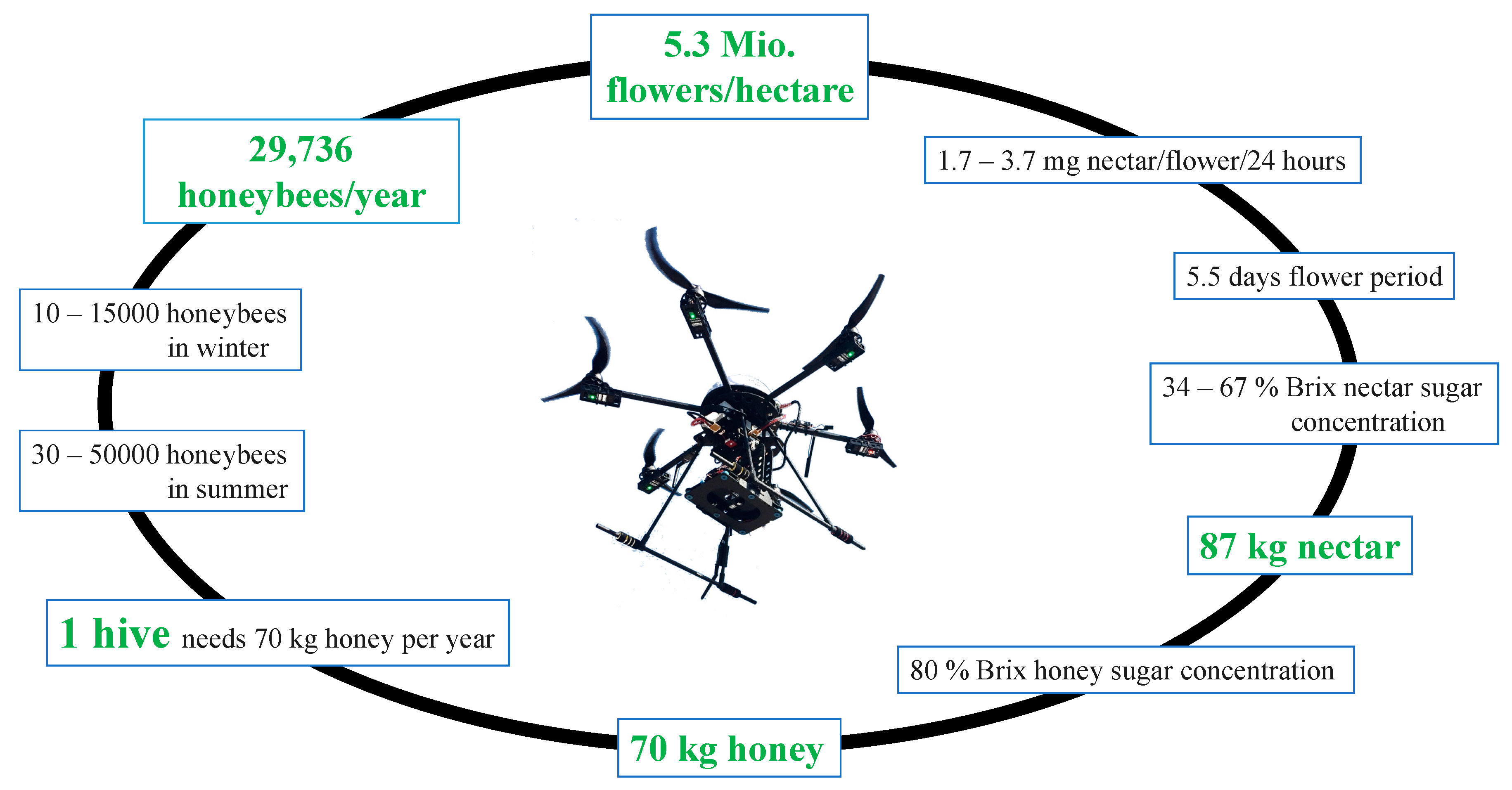
2.2.6. Nectar, Honey, and Honeybees

We use information from the literature [2,84,85,86,87] to estimate the nectar, honey production, and food base for A. mellifera in the study area. R. pseudoacacia blossoms flower for 5.5 days [2]. Black locust produces 1.7–3.7 mg nectar per flower over 24 h, and the nectar has a sugar concentration of 34–67%, so the sugar mass per flower over 24 h is 0.9–2.3 mg, and the honey production reaches 159–1000 kg per hectare [84]. On average, one bee hive requires 70 kg honey per year. In the summer (winter), 30–50,000 (10–15,000) honeybees live in each hive [85,86,87].
Additionally, one week after the flowering period for black locust, we collected the honey of two beekeepers with hives close to the study area. The honey analysis is done in the laboratory (University Hohenheim) and with a refractometer (Brix scale (sugar concentration): 58–90% with a precision 0.5%, Baumé (Bé) 38–43° with 0.5° Bé precision, 12–27% water with 1% precision). Water and sugar concentration and the pollen of both nectar-giving plants and nectarless plants are analyzed in each honey sample.

3. Results

3.1. Vertical Analysis

Figure 3 shows a bird’s-eye view from various FA above the crowns (2.6–92.6 m) with different variables in the blue channel (threshold 110–160). The image shows a decreasing flower surface with increasing FA. The relative flower surface ranges from 2.965% at threshold 110 (shaded and illuminated flowers, some parts of soil) at 2.6 m FA above the crowns to 0.027% threshold 160 (illuminated flowers) at 92.6 m FA above the crowns. The detected area for all FA greater than 42.6 m above crowns covers for each threshold 110–160 similar values such as FA 42.6 m. The strongest signal of decreasing detected flower area occurs at 12.6 m FA above crowns.

3.2. Horizontal Analysis

The analyzed 50 × 50 m2 area is summarized by dividing it into 40 by 80 subareas (Figure 4). Each subarea is represented by a 6.0 × 10.4 m2 grid. The average detected flower area covered 1.33% (threshold 140) out of the total area under study. The minimum (maximum) detected flower area is 0.212% (2.612%). The highest (lowest) flower concentration occurs in field E1 (H1). Figure 4 shows that fewer flowers are present in the southeastern part of the area.

3.3. Flower Trees, Flower Surface, and Volume (2- and 3-Dimensional)

The flower area per Flower Tree detected by the UAV ranges from 242 cm2 to 16,468 cm2 by using threshold 140. A manually count of the number of inflorescences per tree (Table 3) ranges from 84 to 658. On average, 20 flowers are counted per inflorescence. Flowers per tree range from 1913 to 15,559. Tree number two, which was one of the biggest trees in the stand, had a huge number of flowers. Tree two is the highest Flower Tree at 7.2 m (the average tree height was 5.7 m), has the biggest circular crown area of 3.1 m2 (average circular crown area is 1.8 m2) and diameter-at-breast height of 6.0 cm (average diameter-at-breast height is 4.8 cm). Therefore, a significant correlation exists between the greatest tree-size parameters and the highest flower number. For clarity, tree number two is deleted in Figure 5b. The 2D flower surface has a minimum of 0.81 cm2, a mean of 1.92 cm2, and a maximum of 3.26 cm2. The volume or 3D flower surface has a minimum of 3.29 cm3, a mean of 5.96 cm3, and a maximum of 12.19 cm3.
The 2D and 3D flower surfaces of the seven and six (without tree number two) Flower Trees are presented in Figure 5a,b, respectively. The standard error of the 2D flower surface is 7.7 by using all Flower Trees and 3.6 without tree number two. The standard error of the flower volume is 2.3 for all Flower Trees and 1.0 without tree number two. The coefficient of determination for both 2D and 3D measurements is much higher in Figure 5a then in Figure 5b. The detection method was relatively insensitive from 0 to 6000 flowers per tree. Based just on the seven sample trees, no significant correlation appears between flower number and flower surface as detected by the UAV. However, on average the UAV detected 10.86% of the total 2D flower surface and 3.34% of the total 3D flower surface. The average flower surface was 1.92 cm2 (2D), of which 0.21 cm2 were detected by the UAV. In addition, the mean flower volume was 5.96 cm3 (3D), of which 0.20 cm3 were detected by the UAV.

3.4. Flowers, Honey, Apies Mellifera

The two models used to calculate the number of flowers provide very different estimates. Model (1) estimates 11.9 million flowers per hectare and Model (2) uses the arithmetic mean of the horizontal area to estimate 5.3 million flowers per hectare. Using the minimum and maximum percent given by the Horizontal Analysis gives 1.0 to 12.5 million flowers per hectare. Model (1) does not consider flower failure. Model (2) may be used to calibrate Model (1), which overestimates by 56% the number of flowers. The food base for honeybees is calculated by using Model (2) and data from the literature [2,84,85,86,87]. Overall, 5.3 million flowers per hectare may provide 87 kg of nectar (69 kg of honey) and, if just R. pseudoacacia flower, may support a single bee hive for one year (Figure 6).
Honey analysis by refractometer shows 81% Brix honey sugar concentration and 16% water. In the laboratory, the microscopic investigation of pollen (DIN 10760 (a) (A)) [88] (535 and 551 pollen analyzed) reveals that the honey of both beekeepers can be considered R. pseudoacacia (acacia honey). The pollen of nectar-giving and nectarless plants is classified in Table 4. Overall, 19 different nectar-giving plants and 11 different nectarless plants were counted, in addition to R. pseudoacacia, by summing up all the data of honey samples 1 and 2.

4. Discussion

The use of UAVs in agriculture [36,37,38,56,57,62], horticulture [51], plant ecology [66,68,89], and forestry [59,61,62,65] is increasing worldwide. However, UAVs were not heretofore used to quantify the flower production of black locust. In this work, by using a hexacopter and image analysis, we test a method to analyze the flowers of black locust trees in a short-rotation coppice on a previous brown-coal mining area in northeastern Germany. In addition, the flowers of seven sample trees were analyzed manually to calculate the number of flowers and to estimate the nectar and the honey production available as the food base for honeybees.
Based on the UAV and field-collected data, our model estimates 5.3 million flowers at the eight-year-old one-hectare black locust for the year 2017. R. pseudoacacia produces a minimum of 1896 flowers, a mean of 5264 flowers, and a maximum of 15,559 flowers (analysis of Flower Trees). Williams et al. [90] analyzed Eucalyptus nitens flowers in Tasmania and found a minimum of 8 flowers per tree and a maximum of 211 flowers per tree [90]. The flower production of R. pseudoacacia is high compared with that of E. nitens, but the flowers of R. pseudoacacia are smaller than those of E. nitens and the flower-insect relationships differ between the two tree species. Furthermore, E. nitens flowers for three months (from January to March) [91], whereas R. pseudoacacia flowers only 5.5 days [2]. Williams et al. [90] counted flowers manually. An additional analysis done with the aid of UAVs would have been possible because the white color of E. nitens flowers differs significantly from the colors of other elements, such as leaves, and branches, and rocks.
In the present study, 11% of the total 2D surface and 5.5% of the total volume (3D) of the R. pseudoacacia flower area are captured by the UAV. For future studies, we recommend analyzing more than seven flower trees to obtain a more accurate coefficient of determination (regression) and more significant correlations between flower number and detected flower area. Horton et al. [51] obtained an average detection success rate of 84.3% for peach flowers. However, peach plantations have the advantage that the trees flower before foliation. In addition, the stand density is lower, and the peach trees are smaller than black locust trees. Horton et al. [51] explains that some of the white and light-pink flowers are similar in color to the branches and some parts of the ground. In Germany, R. pseudoacacia normally flower at the end of May after foliation. Therefore, many flowers are concealed by leaves, branches, or other flowers.
Near-infrared cameras were useful for collecting debilitation of plants caused by nutrient deficiency (potassium) or insect attacks (green peach aphid or bark beetle) and for calculating the normalized density vegetation index [37,59,61,92]. In the present study, the blue channel is used to analyze the flowers in the UAV pictures. This corresponds to the description of Horton et al. [51]: objects with high chlorophyll (weeds) reflect strongly in the near-infrared and green bands but poorly in the blue band. In our study, because of the chlorophyll, the leaves reflect strongly in the near-infrared and green bands. In the blue channel, the biomass (chlorophyll) reflects poorly, but the white flowers reflect strongly. Therefore, a noticeable boundary exists between flower and tree (and weed) biomass. Richardson et al. [34] used the relative brightness of the red channel (red%) to analyze flowers of red maple trees. Because the flowers of red maple trees are red, the best boundary is obtained by using the red channel. Overall, flower analysis is possible in most cases with a RGB camera. The use of the blue channel to analyze the flowers of black locust works well. We tested various thresholds in the blue channel (110–160). Shaded and illuminated flowers (and some parts of the soil) are detected at threshold 110, whereas only illuminated flowers are detected at threshold 160. Consequently, at threshold 160 the User Accuracy Flower and the Producer Accuracy Biomass were 100%. However, 46.6% from the flowers are detected as biomass and get lost for the calculations (Appendix A, Table A1). When comparing all thresholds, threshold 140 performed best with respect to Overall Accuracy and Kappa Coefficient [77,78] and was therefore used in Horizontal and Flower Tree analyses to measure the flower area.
The Vertical Analyses are similar to that applied by Severtson et al. [37] with the vertical FA ranging from 20 to 110 m above the starting point. The flower surface of the entire area (leaves, branches, stones, soil, etc.) ranges from 2.97% to 0.03% at FAs of 2.6 and 92.6 m above the crowns, respectively. This indicates that flowers occupy just a small fraction of the environment in black locust plantations, and that most flowers are detectable if the UAV flies as near as possible to the crowns. As of 12.6 m FA above crowns, the detected flower area decreases rapidly. The size of the flowers does not change, but the area monitored by the UAV increases. The GSD changes rapidly with increasing FA. Therefore, the white color of the flowers merges with the darker colors of the leaves, branches, weed, and soil. Consequently, the threshold per pixel decreases. The detected area remains essentially constant for all FAs greater than 50 m above the starting point. Radiometric calibration is not applied, because radiometric distortions, normally caused by atmospheric influences, were insignificant considering the very low FAs [61,93]. Furthermore, the detected area does not significantly increase if the flower number increases from 0 to 6000 flowers per tree: the number of flowers detected remains nearly constant, except for tree number 2 of 60% detected flower area. Tree number 2 had a large number of flowers (15,000 flowers per tree) compared with the other Flower Trees. Tree 2 was not in a different phenological state as the other trees. One explanation for the recognized large number of flowers and area is; tree 2 was one of the biggest (diameter, height, circular crown area) trees in the stand. Higher trees tree might benefit more from sun light for energy production, and the bigger circular crown area indicates a high number of branches that can produce more flowers altogether. The use of the crown-correction factor is advised if the ground-slope angle is greater than 10°, but it is also important if the tree height varies along and between the lines in the study area. Therefore, the crown-correction factor is one possible way to improve the precision of the results. Tree growth rate varies from tree to tree, which leads to variations in tree height, branches, and crown structure.
Model (2) of this study estimates 5.3 million flowers for one hectare of eight-year-old R. pseudoacacia plantation. As a result, one bee hive could survive one year from the estimated honey base. In the previous brown-coal mining area of Lauchhammer, 40 hectares were planted with R. pseudoacacia over the last 10 years. Moreover, older black locust forests and black locust in mixed stands are neighboring to the study area. Therefore, at least 40 A. mellifera hives could survive, if all replanted areas (40 hectare) have nearly the same number of flowers as the study area. In these times of loss of biodiversity [94,95,96,97], this study shows that re-planting of human dispelled landscape, such as former mining areas, can be beneficial to the food base, especially for honeybees. To understand the relationships between flower production and stand density, tree age, tree diameter, and tree height, further studies in different areas are recommended.
The estimated honey base of this study is 70 kg per hectare, which is the honey mass required per year for an average A. mellifera hive [85]. However, 70 kg per hectare is scant, compared with results from Hungary. In Hungary, nectar and honey yield of black locust is increases from year 6 to year 15. The maximum nectar yield is 836 kg/ha of nectar and 418 kg/ha of honey. The lowest yield is documented for year 36 with 384 kg/ha of nectar and 192 kg/ha of honey [3]. These results of Hungarian scientists are consistent with those of Droege [84], who reports that honey production of R. pseudoacacia ranges from 195 to 1000 kg/ha. Therefore, the 70 kg/ha calculated in this study is lower than the lowest limit of Droege [84] (195 kg/ha). This results may be attributed to the cold weather that occurred in mid-April 2017; with frost on 16 and 17 April 2017. In addition, the weather was not optimal during flower time. On 30 May, a thunderstorm destroyed some flowers. Surprisingly, beekeepers in Germany and the authors of this study observed more than one flowering period in 2017. In some areas in the south and the middle of Germany black locust flowered in mid-June and again at end of August. Further studies and observations are thus needed to get an overview of this behavior and to find mechanism behind it. However, the main flowering period is the end of May and one of the big challenges of flower analysis and honey production of black locust, especially for scientists, but also for non-local beekeepers, is the short time during of the flowering period, which lasts on average 5.5 days [2]. One week after the main flowering period of R. pseudoacacia our two beekeepers extracted the honey from their hives. The laboratory of the University of Hohenheim classified the honey as R. pseudoacacia honey. However, a microscopic pollen investigation revealed 30 different pollens of nectar-giving and nectarless plants in the two honey samples. These results show that, during the flowering time of R. pseudoacacia, a lot of other plant species produced energy spending flowers or pollen for honeybees. The focus of this study has been on a monoculture (plantation). However, biodiversity and ecosystem health benefits from the presence of many different plant species, and animal species as part of the biocoenosis of the ecosystem. Thus, the analysis of flowers is important to understand ecosystems worldwide.
Natural scientists, researcher, politicians, and layman are constantly learning more about the sensitivity of the environment from the results of UAV-based analyses. UAV technology is a sustainable technology that provides high-resolution analyses and minimal environmental damage. Therefore, the methodology of this study and of other studies [39,51,52,65] should be further tested to determine whether it is applicable to other tree species of differing ages and in mixed-forest stands. One hypothesis is that older trees probably have a different vertical crown structure (more branch layers) and thus contribute a different proportion of captured flowers. In mixed-forest stands, different tree species are part of the community and have differing flowering times during the year and different flowering-time durations. Flower analysis is difficult in complex ecosystems but provides an interesting indicator of the plant-animal (tree-insect) relationship, ecosystem health, and biodiversity.

5. Conclusions

This study proposes a methodology to analyze flowers in tree plantations and tested the method by applying it to an eight-year-old R. pseudoacacia plantation in a former mining area in Germany. The flower analysis was done by using images acquired by a UAV that were analyzed with the aid of the image analyzing software ImageJ. Seven Flower Trees were manually accessed to obtain reference data. Overall, most flowers are detectable if the UAV flies as near as possible to the crowns. The vertical flying analysis shows that the flower area is 2.97% (threshold 110), and 1.33% (threshold 140) at 2.6 m FA above the crowns, and 0.03% (threshold 160) at 92.6 m. The UAV captured 11% of the 2D flower surface and 3% of the flower volume (3D) of R. pseudoacacia flowers. Thus, the model estimates 5.3 million flowers are present in the analyzed one-hectare black locust plantation. On average, one honeybee hive could survive one year from the 2017 analyzed flowers of the one-hectare area of black locust.
The methodology and results presented herein provide local managers, foresters, and scientists with the opportunity to estimate flower productivity of black locust and further tree species worldwide. This study demonstrates that RGB images acquired by UAVs can be used effectively to obtain rapid, economical, and meaningful estimates of flowers, nectar, honey production, and honeybee potential.

Acknowledgments

This research has been supported by the University of Applied Science Erfurt (FHE) and the Technical University of Munich (TUM). Further, this work was supported by the German Research Foundation (DFG) and the Technical University of Munich (TUM) in the framework of the Open Access Publishing Program. We thank the company Lausitzer und Mitteldeutsche Bergbau–Verwaltungsgesellschaft (LMBV) for their support to analyze the study area. The authors are also grateful to thank Axel Weckschmied (Hexapilots®) for a very well flying performance of his hexacopter. Thanks to Christian Wolf and the store Alte Schäferei-Bockwitz for honey jar samples, and the laboratory of the University Hohenheim for honey analysis. We thank Tobias Clauß, Christian Clauß, and Jan Tumajer for initial ideas for image analysis, as well as Petra Clauß for statistical support. We are very happy for the assistance of Jan Zimmermanns during the field data collection, and proofreading by Daniela Carl, Astrid Moser, Jan Tumajer, and English Editing Service Enago. The comments of two anonymous reviewers were helpful to improve an earlier version of the manuscript.

Author Contributions

Hans Pretzsch, Dirk Landgraf and Christin Carl initiated and planned the project; Christin Carl performed the experiments, analyzed the data with Peter Biber, and wrote the manuscript. Dirk Landgraf, Peter Biber, Marieke van der Maaten-Theunissen and Hans Pretzsch, contributed by revising the manuscript.

Conflicts of Interest

The authors declare no conflict of interest.

Abbreviations

The following abbreviations are used in this manuscript:
2DTwo-Dimensional, flower surface area
3DThree-Dimensional, flower volume
FAFlying Altitude
FoAFlower Area
FOVField of View
FSUAverage flower Surface detected by UAV
GSDGround Sample Distance
LAILeaf Area Index
RGBRed-Green-Blue
UAVUnmanned Aerial Vehicles

Appendix A

Figure A1. Real flying altitude above starting point measured by UAV on-board computer (A), above ground (B), and above crown (C): distance to rocks (a), slope angle (α), distance between the lines (b), tree height (c), angle and slope between two tree crowns ( ε ). All in-field measurements are in green and the calculated values are in red.
Remotesensing 09 01091 g007
The real FA above ground (B) is calculated by using the FA from the starting point (A) minus the distance to rocks ( a ):
B = A a
Therefore, a is calculated by using the slope angle (α) and distance between the lines (b) for each line analyzed (Figure A1):
a = bsin ( α )
Scale bars were placed on the ground in the forest stand (Vertical and Horizontal Analysis). When calculating the flower area, the scale bar should be adapted to the crowns, where the flowers are located. Therefore, the FA above the crowns (C) is calculated from the FA above the ground (B) minus the tree heights (c):
C = B c
The real size of the scale bars (d) is calculated by using the real FA above ground (B) and the viewing angle (β):
d = 2 ( B cos ( β 2 ) ) 2 B 2
To calculate the viewing angle (β) the FA above the crowns (C) and scale bar at the floor (e) are needed:
β = 2 arctan ( e / 2 C )
Because the flowers are located in the crowns and the slopes of the crowns differ, a crown-correction factor (D) for the pictures is obtained by using the crown angles (ε):
D = 1 cos ( ε )
Input data for the crown angle are the angle of the ground slope (α), the distance between trees (b), and the tree height (c) (Figure A1). Moreover, the difference in height between trees in the first line (c1), and in the second line (c2), and so on is calculated:
ε = α + arctan ( c 2 c 1 b )
Table A1. Accuracy assessment of flower detection by UAV in 3 m flying altitude above crowns. Therefore 12,500 pixels were analyzed (ImageJ segmentation versus user/visual inspection of flowers) and two classes were used: Flower and Biomass. In the blue channel for six different thresholds is calculated the Overall Accuracy, the Producer Accuracy (Omission Error), the Users Accuracy (Commission Error), the Mean Accuracy, and the Kappa Coefficient.
ThresholdOverall Accuracy (%)Producers Accuracy (Flower)Producers Accuracy (Biomass)Users Accuracy (Flower)Users Accuracy (Biomass)Mean Accuracy (%)Kappa Coefficient
>11098.610098.566.210090.80.789
>12099.199.499.175.599.993.40.854
>13099.497.099.584.399.995.70.899
>14099.589.299.894.099.798.20.913
>15099.270.799.999.299.199.20.822
>16098.753.410010098.799.00.690

References

  1. European Commission under the Sixth Framework Programme through the DAISIE Project. Delivering Alien Invasive Species Inventories for Europe—Species Factsheet Robinia Pseudoacacia. Available online: http://www.europe-aliens.org/speciesFactsheet.do?speciesId=11942 (accessed on 29 June 2017).
  2. Roloff, A.; Weisgerber, H.; Lang, U.; Stimm, B. Bäume Nordamerikas—Von Alligator-Wachholder bis Zuckerahorn. Alle Charakteristischen Arten im Porträt; Wiley-VCH Verlag GmbH & Co. KGaA: Weinheim, Germany, 2010; ISBN 978-3-527-32825-3. [Google Scholar]
  3. Rédei, K. Black Locust (Robinia pseudoacacia L.) Growing in Hungary; Hungarian Forest Research Institute: Sarvar, Hungary, 2013; pp. 72–73. [Google Scholar]
  4. Deutscher Imkerverbund e.V. Honigsorten-Bezeichnungen. Available online: http://deutscherimkerbund.de/userfiles/downloads/satzung_richtlinien/Merkblatt_Sorten_3_4_neu.pdf (accessed on 19 July 2017).
  5. Rogan, J.; Franklin, J.; Roberts, D.A. A comparison of methods for monitoring multitemporal vegetation change using Thematic Mapper imagery. Remote Sens. Environ. 2002, 80, 143–156. [Google Scholar] [CrossRef]
  6. Tucker, C.J. Red and photographic infrared linear combinations for monitoring vegetation. Remote Sens. Environ. 1979, 8, 127–150. [Google Scholar] [CrossRef]
  7. Knipling, E.B. Physical and physiological basis for the reflectance of visible and near-infrared radiation from vegetation. Remote Sens. Environ. 1970, 1, 155–159. [Google Scholar] [CrossRef]
  8. Gitelson, A.A.; Kaufman, Y.J.; Stark, R.; Rundquist, D. Novel algorithms for remote estimation of vegetation fraction. Remote Sens. Environ. 2002, 80, 76–87. [Google Scholar] [CrossRef]
  9. Qi, J.; Chehbouni, A.; Huete, A.R.; Kerr, Y.H.; Sorooshian, S. A modified soil adjusted vegetation index. Remote Sens. Environ. 1994, 48, 119–126. [Google Scholar] [CrossRef]
  10. Jiang, H.; Chen, S.; Li, D.; Wang, C.; Yang, J. Papaya Tree Detection with UAV Images Using a GPU-Accelerated Scale-Space Filtering Method. Remote Sens. 2017, 9, 721. [Google Scholar] [CrossRef]
  11. Asner, G.P. Biophysical and biochemical sources of variability in canopy reflectance. Remote Sens. Environ. 1998, 64, 234–253. [Google Scholar] [CrossRef]
  12. Baret, F.; Clevers, J.G.P.W.; Steven, M.D. The robustness of canopy gap fraction estimates from red and near-infrared reflectances: A comparison of approaches. Remote Sens. Environ. 1995, 54, 141–151. [Google Scholar] [CrossRef]
  13. Le Maire, G.; François, C.; Soudani, K.; Berveiller, D.; Pontailler, J.Y.; Bréda, N.; Genet, H.; Davi, H.; Dufrêne, E. Calibration and validation of hyperspectral indices for the estimation of broadleaved forest leaf chlorophyll content, leaf mass per area, leaf area index and leaf canopy biomass. Remote Sens. Environ. 2008, 112, 3846–3864. [Google Scholar] [CrossRef]
  14. Gower, S.T.; Kucharik, C.J.; Norman, J.M. Direct and indirect estimation of leaf area index, fAPAR, and net primary production of terrestrial ecosystems. Remote Sens. Environ. 1999, 70, 29–51. [Google Scholar] [CrossRef]
  15. Hu, J.; Su, Y.; Tan, B.; Huang, D.; Yang, W.; Schull, M.; Bull, M.A.; Martonchik, J.V.; Diner, D.J.; Knyazikhin, Y.; et al. Analysis of the MISR LAI/FPAR product for spatial and temporal coverage, accuracy and consistency. Remote Sens. Environ. 2007, 107, 334–347. [Google Scholar] [CrossRef]
  16. Turner, D.P.; Cohen, W.B.; Kennedy, R.E.; Fassnacht, K.S.; Briggs, J.M. Relationships between leaf area index and Landsat TM spectral vegetation indices across three temperate zone sites. Remote Sens. Environ. 1999, 70, 52–68. [Google Scholar] [CrossRef]
  17. North, P.R. Estimation of f APAR, LAI, and vegetation fractional cover from ATSR-2 imagery. Remote Sens. Environ. 2002, 80, 114–121. [Google Scholar] [CrossRef]
  18. Demarez, V.; Gastellu-Etchegorry, J.P. A modeling approach for studying forest chlorophyll content. Remote Sens. Environ. 2000, 71, 226–238. [Google Scholar] [CrossRef]
  19. Houborg, R.; Boegh, E. Mapping leaf chlorophyll and leaf area index using inverse and forward canopy reflectance modeling and SPOT reflectance data. Remote Sens. Environ. 2008, 112, 186–202. [Google Scholar] [CrossRef]
  20. Healey, S.P.; Cohen, W.B.; Zhiqiang, Y.; Krankina, O.N. Comparison of Tasseled Cap-based Landsat data structures for use in forest disturbance detection. Remote Sens. Environ. 2005, 97, 301–310. [Google Scholar] [CrossRef]
  21. Hilker, T.; Wulder, M.A.; Coops, N.C.; Linke, J.; McDermid, G.; Masek, J.G.; Gao, F.; White, J.C. A new data fusion model for high spatial-and temporal-resolution mapping of forest disturbance based on Landsat and MODIS. Remote Sens. Environ. 2009, 113, 1613–1627. [Google Scholar] [CrossRef]
  22. Meddens, A.J.; Hicke, J.A.; Vierling, L.A. Evaluating the potential of multispectral imagery to map multiple stages of tree mortality. Remote Sens. Environ. 2011, 115, 1632–1642. [Google Scholar] [CrossRef]
  23. Bright, B.C.; Hicke, J.A.; Hudak, A.T. Estimating aboveground carbon stocks of a forest affected by mountain pine beetle in Idaho using lidar and multispectral imagery. Remote Sens. Environ. 2012, 124, 270–281. [Google Scholar] [CrossRef]
  24. Cheng, T.; Rivard, B.; Sánchez-Azofeifa, G.A.; Feng, J.; Calvo-Polanco, M. Continuous wavelet analysis for the detection of green attack damage due to mountain pine beetle infestation. Remote Sens. Environ. 2010, 114, 899–910. [Google Scholar] [CrossRef]
  25. Coops, N.C.; Johnson, M.; Wulder, M.A.; White, J.C. Assessment of QuickBird high spatial resolution imagery to detect red attack damage due to mountain pine beetle infestation. Remote Sens. Environ. 2006, 103, 67–80. [Google Scholar] [CrossRef]
  26. Dennison, P.E.; Brunelle, A.R.; Carter, V.A. Assessing canopy mortality during a mountain pine beetle outbreak using GeoEye-1 high spatial resolution satellite data. Remote Sens. Environ. 2010, 114, 2431–2435. [Google Scholar] [CrossRef]
  27. DeRose, R.J.; Long, J.N.; Ramsey, R.D. Combining dendrochronological data and the disturbance index to assess Engelmann spruce mortality caused by a spruce beetle outbreak in southern Utah, USA. Remote Sens. Environ. 2011, 115, 2342–2349. [Google Scholar] [CrossRef]
  28. Meddens, A.J.; Hicke, J.A.; Vierling, L.A.; Hudak, A.T. Evaluating methods to detect bark beetle-caused tree mortality using single-date and multi-date Landsat imagery. Remote Sens. Environ. 2013, 132, 49–58. [Google Scholar] [CrossRef]
  29. Meigs, G.W.; Kennedy, R.E.; Cohen, W.B. A Landsat time series approach to characterize bark beetle and defoliator impacts on tree mortality and surface fuels in conifer forests. Remote Sens. Environ. 2011, 115, 3707–3718. [Google Scholar] [CrossRef]
  30. Skakun, R.S.; Wulder, M.A.; Franklin, S.E. Sensitivity of the thematic mapper enhanced wetness difference index to detect mountain pine beetle red-attack damage. Remote Sens. Environ. 2003, 86, 433–443. [Google Scholar] [CrossRef]
  31. White, J.C.; Wulder, M.A.; Brooks, D.; Reich, R.; Wheate, R.D. Detection of red attack stage mountain pine beetle infestation with high spatial resolution satellite imagery. Remote Sens. Environ. 2005, 96, 340–351. [Google Scholar] [CrossRef]
  32. Landmann, T.; Piiroinen, R.; Makori, D.M.; Abdel-Rahman, E.M.; Makau, S.; Pellikka, P.; Raina, S.K. Application of hyperspectral remote sensing for flower mapping in African savannas. Remote Sens. Environ. 2015, 166, 50–60. [Google Scholar] [CrossRef]
  33. Abdel-Rahman, E.M.; Makori, D.M.; Landmann, T.; Piiroinen, R.; Gasim, S.; Pellikka, P.; Raina, S.K. The utility of AISA eagle hyperspectral data and random forest classifier for flower mapping. Remote Sens. 2015, 7, 13298–13318. [Google Scholar] [CrossRef]
  34. Richardson, A.D.; Braswell, B.H.; Hollinger, D.Y.; Jenkins, J.P.; Ollinger, S.V. Near-surface remote sensing of spatial and temporal variation in canopy phenology. Ecol. Appl. 2009, 19, 1417–1428. [Google Scholar] [CrossRef] [PubMed]
  35. Walter, A.; Finger, R.; Huber, R.; Buchmann, N. Opinion: Smart farming is the key to developing sustainable agriculture. Proc. Natl. Acad. Sci. USA 2017, 114, 6148–6150. [Google Scholar] [CrossRef] [PubMed]
  36. Calvario, G.; Sierra, B.; Alarcón, T.E.; Hernandez, C.; Dalmau, O. A Multi-Disciplinary Approach to Remote Sensing through Low-Cost UAVs. Sensors 2017, 17, 1411. [Google Scholar] [CrossRef] [PubMed]
  37. Severtson, D.; Callow, N.; Flower, K.; Neuhaus, A.; Olejnik, M.; Nansen, C. Unmanned aerial vehicle canopy reflectance data detects potassium deficiency and green peach aphid susceptibility in canola. Precis. Agric. 2016, 17, 659–677. [Google Scholar] [CrossRef]
  38. Fang, S.; Tang, W.; Peng, Y.; Gong, Y.; Dai, C.; Chai, R.; Liu, K. Remote estimation of vegetation fraction and flower fraction in oilseed rape with unmanned aerial vehicle data. Remote Sens. 2016, 8, 416. [Google Scholar] [CrossRef]
  39. Gnädinger, F.; Schmidhalter, U. Digital Counts of Maize Plants by Unmanned Aerial Vehicles (UAVs). Remote Sens. 2017, 9, 544. [Google Scholar] [CrossRef]
  40. Maresma, Á.; Ariza, M.; Martínez, E.; Lloveras, J.; Martínez-Casasnovas, J.A. Analysis of vegetation indices to determine nitrogen application and yield prediction in maize (Zea mays L.) from a standard UAV service. Remote Sens. 2016, 8, 973. [Google Scholar] [CrossRef]
  41. Roosjen, P.P.; Suomalainen, J.M.; Bartholomeus, H.M.; Kooistra, L.; Clevers, J.G. Mapping Reflectance Anisotropy of a Potato Canopy Using Aerial Images Acquired with an Unmanned Aerial Vehicle. Remote Sens. 2017, 9, 417. [Google Scholar] [CrossRef]
  42. Roosjen, P.P.; Suomalainen, J.M.; Bartholomeus, H.M.; Clevers, J.G. Hyperspectral Reflectance Anisotropy Measurements Using a Pushbroom Spectrometer on an Unmanned Aerial Vehicle—Results for Barley, Winter Wheat, and Potato. Remote Sens. 2016, 8, 909. [Google Scholar] [CrossRef]
  43. Schirrmann, M.; Giebel, A.; Gleiniger, F.; Pflanz, M.; Lentschke, J.; Dammer, K.H. Monitoring Agronomic Parameters of Winter Wheat Crops with Low-Cost UAV Imagery. Remote Sens. 2016, 8, 706. [Google Scholar] [CrossRef]
  44. Du, M.; Noguchi, N. Monitoring of Wheat Growth Status and Mapping of Wheat Yield’s within-Field Spatial Variations Using Color Images Acquired from UAV-camera System. Remote Sens. 2017, 9, 289. [Google Scholar] [CrossRef]
  45. Holman, F.H.; Riche, A.B.; Michalski, A.; Castle, M.; Wooster, M.J.; Hawkesford, M.J. High throughput field phenotyping of wheat plant height and growth rate in field plot trials using UAV based remote sensing. Remote Sens. 2016, 8, 1031. [Google Scholar] [CrossRef]
  46. Yue, J.; Yang, G.; Li, C.; Li, Z.; Wang, Y.; Feng, H.; Xu, B. Estimation of Winter Wheat Above-ground Biomass Using Unmanned Aerial Vehicle-based Snapshot Hyperspectral Sensor and Crop Height Improved Models. Remote Sens. 2017, 9, 708. [Google Scholar] [CrossRef]
  47. Burkart, A.; Aasen, H.; Alonso, L.; Menz, G.; Bareth, G.; Rascher, U. Angular dependency of hyperspectral measurements over wheat characterized by a novel UAV based goniometer. Remote Sens. 2015, 7, 725–746. [Google Scholar] [CrossRef] [Green Version]
  48. Luna, I.; Lobo, A. Mapping Crop Planting Quality in Sugarcane from UAV Imagery: A Pilot Study in Nicaragua. Remote Sens. 2016, 8, 500. [Google Scholar] [CrossRef]
  49. Mathews, A.J.; Jensen, J.L. Visualizing and quantifying vineyard canopy LAI using an unmanned aerial vehicle (UAV) collected high density structure from motion point cloud. Remote Sens. 2013, 5, 2164–2183. [Google Scholar] [CrossRef]
  50. Matese, A.; Toscano, P.; Di Gennaro, S.F.; Genesio, L.; Vaccari, F.P.; Primicerio, J.; Belli, C.; Zaldei, A.; Bianconi, A.; Gioli, B. Intercomparison of UAV, aircraft and satellite remote sensing platforms for precision viticulture. Remote Sens. 2015, 7, 2971–2990. [Google Scholar] [CrossRef]
  51. Horton, R.; Cano, E.; Bulanon, D.; Fallahi, E. Peach Flower Monitoring Using Aerial Multispectral Imaging. J. Imaging 2017, 3, 2. [Google Scholar] [CrossRef]
  52. Fernández, T.; Pérez, J.L.; Cardenal, J.; Gómez, J.M.; Colomo, C.; Delgado, J. Analysis of landslide evolution affecting olive groves using uav and photogrammetric techniques. Remote Sens. 2016, 8, 837. [Google Scholar] [CrossRef]
  53. Ortega-Farías, S.; Ortega-Salazar, S.; Poblete, T.; Kilic, A.; Allen, R.; Poblete-Echeverría, C.; Ahumada-Orellana, L.; Zuñiga, M.; Sepúlveda, D. Estimation of energy balance components over a drip-irrigated olive orchard using thermal and multispectral cameras placed on a helicopter-based unmanned aerial vehicle (UAV). Remote Sens. 2016, 8, 638. [Google Scholar] [CrossRef]
  54. Díaz-Varela, R.A.; de la Rosa, R.; León, L.; Zarco-Tejada, P.J. High-resolution airborne UAV imagery to assess olive tree crown parameters using 3D photo reconstruction: Application in breeding trials. Remote Sens. 2015, 7, 4213–4232. [Google Scholar] [CrossRef]
  55. Jiang, Z.; Huete, A.R.; Didan, K.; Miura, T. Development of a two-band enhanced vegetation index without a blue band. Remote Sens. Environ. 2008, 112, 3833–3845. [Google Scholar] [CrossRef]
  56. Hexapilots, Unmanned Aerial Services. Available online: http://wm1bc4730.homepage.t-online.de/hexawp/ (accessed on 13 May 2017).
  57. Apus Systems Intelligent Geocoding. Available online: https://www.apus-systems.com (accessed on 25 July 2017).
  58. Mund, J.-P.; Cremer, T.; Krause, S. Potenzial und Perspektive: Drohnen in der Forstwirtschaft. AFZ DerWald 2017, 17, 43–46. [Google Scholar]
  59. Festmeter—Ihr Wald. Available online: http://www.festmeter.at (accessed on 12 May 2017).
  60. Näsi, R.; Honkavaara, E.; Lyytikäinen-Saarenmaa, P.; Blomqvist, M.; Litkey, P.; Hakala, T.; Viljanen, N.; Kantola, T.; Tanhuanpää, T.; Holopainen, M. Using UAV-based photogrammetry and hyperspectral imaging for mapping bark beetle damage at tree-level. Remote Sens. 2015, 7, 15467–15493. [Google Scholar] [CrossRef]
  61. Lehmann, J.R.K.; Nieberding, F.; Prinz, T.; Knoth, C. Analysis of unmanned aerial system-based CIR images in forestry—A new perspective to monitor pest infestation levels. Forests 2015, 6, 594–612. [Google Scholar] [CrossRef] [Green Version]
  62. Rucon Engineering, Über RUCON Engineering. Available online: http://rucon.de (accessed on 20 March 2017).
  63. Duan, F.; Wan, Y.; Deng, L. A Novel Approach for Coarse-to-Fine Windthrown Tree Extraction Based on Unmanned Aerial Vehicle Images. Remote Sens. 2017, 9, 306. [Google Scholar] [CrossRef]
  64. Sohns, V. LIGNA 2017 zeigt Forsttechnik und Produktionskette. AFZ DerWald 2017, 13, 35–37. [Google Scholar]
  65. Eusemann, P.; Liesebach, M.; Liesebach, H. Mit Drohnen Ernteaussichten in Saatgutbeständen erkunden. AFZ DerWald 2017, 10, 28–30. [Google Scholar]
  66. Chianucci, F.; Disperati, L.; Guzzi, D.; Bianchini, D.; Nardino, V.; Lastri, C.; Rindinella, A.; Corona, P. Estimation of canopy attributes in beech forests using true colour digital images from a small fixed-wing UAV. Int. J. Appl. Earth Obs. Geoinform. 2016, 47, 60–68. [Google Scholar] [CrossRef] [Green Version]
  67. Cunliffe, A.M.; Brazier, R.E.; Anderson, K. Ultra-fine grain landscape-scale quantification of dryland vegetation structure with drone-acquired structure-from-motion photogrammetry. Remote Sens. Environ. 2016, 183, 129–143. [Google Scholar] [CrossRef] [Green Version]
  68. McNeil, B.E.; Pisek, J.; Lepisk, H.; Flamenco, E.A. Measuring leaf angle distribution in broadleaf canopies using UAVs. Agric. For. Meteorol. 2016, 218, 204–208. [Google Scholar] [CrossRef]
  69. MacInnis, G.; Forrest, J. Quantifying pollen deposition with macro photography and ‘stigmagraphs’. J. Pollinat. Ecol. 2017, 20, 13–21. [Google Scholar]
  70. Lino, A.C.L.; Sanches, J.; Moraes, G.; Dias-Tagliacozzo, I.M.D.; Augusto, F.; Lima, B.; Nascimento, T.S. Flower classification supported by digital imaging techniques. J. Inform. Technol. Agric. 2011, 4, 1–6. [Google Scholar]
  71. Deutscher Wetterdienst DWD. Archiv Monats- und Tageswerte. Available online: http://www.dwd.de (accessed on 10 June 2017).
  72. Landgraf, D.; Böcker, L.; Wiesner, S.; Kempe, K. Energiewald Kostebrau—Chancen und Risiken für die Stadt Lauchhammer. In Proceedings of the Tagungsband zur Fachtagung Anbau und Nutzung von Bäumen auf landwirtschaftlichen Flächen, Freiburg, Germany, 3 July 2007; pp. 39–45. [Google Scholar]
  73. yWorks, the Diagramming Company. Available online: http://www.yworks.com/products/yed/download (accessed on 20 January 2017).
  74. MAPIR—Survey2 Camera—Visible Light RGB. Available online: https://www.mapir.camera/products/survey2-camera-visible-light-rgb (accessed on 28 May 2017).
  75. Schneider, C.A.; Rasband, W.S.; Eliceiri, K.W. NIH Image to ImageJ: 25 years of image analysis. Nat. Methods 2012, 9, 671–675. [Google Scholar] [CrossRef] [PubMed]
  76. Schindelin, J.; Arganda-Carreras, I.; Frise, E. Fiji: An open-source platform for biological-image analysis. Nat. Methods 2012, 9, 676–682. [Google Scholar] [CrossRef] [PubMed]
  77. Grouven, U.; Bender, R.; Ziegler, A.; Lange, S. Der kappa-koeffizient. Dtsch. Med. Wochenschr. 2007, 132, e65–e68. [Google Scholar] [CrossRef] [PubMed]
  78. Landis, J.R.; Koch, G.G. The measurement of observer agreement for categorical data. Biometrics 1977, 33, 159–174. Available online: https://pdfs.semanticscholar.org/7e73/43a5608fff1c68c5259db0c77b9193f1546d.pdf (accessed on 18 October 2017). [CrossRef] [PubMed]
  79. R Core Team. R: A Language and Environment for Statistical Computing. R Foundation for Statistical Computing, Vienna, Austria. 2016. Available online: https://www.R-project.org/ (accessed on 23 November 2016).
  80. Paradis, E.; Claude, J.; Strimmer, K. APE: Analyses of phylogenetics and evolution in R language. Bioinformatics 2004, 20, 289–290. [Google Scholar] [CrossRef] [PubMed]
  81. Wickham, H. ggplot2: Elegant Graphics for Data Analysis; Springer-Verlag: New York, NY, USA, 2009. [Google Scholar]
  82. Urbanek, S. png: Read and Write PNG Images. R Package Version 0.1–7. Available online: https://CRAN.R-project.org/package=png (accessed on 3 July 2017).
  83. Murrell, P. gridGraphics: Redraw Base Graphics Using ‘Grid’ Graphics. R Package Version 0.2. 2017. Available online: https://CRAN.R-project.org/package=gridGraphics (accessed on 3 July 2017).
  84. Droege, G. Das Imkerbuch; VEB Deutscher Landwirtschaftsverlag: Berlin, Germany, 1989; p. 106. ISBN 3331002623. [Google Scholar]
  85. Dachmarke—Über Bienen und Honig. Available online: http://dachmarke.com/produkte/bienenwissen/ (accessed on 25 June 2017).
  86. Die Honigmacher. Winterbiene. Available online: http://www.die-honigmacher.de/kurs3/seite_15103.html (accessed on 20 June 2017).
  87. Imkerverein Büchertal. Biologie des Bienenvolkes. Available online: http://www.imkerverein-buechertal.de/Biologie_Bienenvolk.php (accessed on 20 May 2017).
  88. Deutsches Institut für Normung e. V. Untersuchung von Honig—Bestimmung der Relativen Pollenhaüfigkeit, DIN 10760. 2002, pp. 1–6. Available online: https://www.din.de/de/mitwirken/normenausschuesse/krdl/din-spec/wdc-beuth:din21:47633680 (accessed on 13 September 2017).
  89. Cruzan, M.B.; Weinstein, B.G.; Grasty, M.R.; Kohrn, B.F.; Hendrickson, E.C.; Arredondo, T.M.; Thompson, P.G. Small unmanned aerial vehicles (micro-UAVs, drones) in plant ecology. Appl. Plant Sci. 2016, 4, 1600041. [Google Scholar] [CrossRef] [PubMed]
  90. Williams, D.R.; Potts, B.M.; Neilsen, W.A.; Joyce, K.R. The effect of tree spacing on the production of flowers in Eucalyptus nitens. Aust. For. 2006, 69, 299–304. [Google Scholar] [CrossRef]
  91. Yarra Ranges Shire Council, Eucalyptus Nitens. Available online: http://fe.yarraranges.vic.gov.au/Residents/Trees_Vegetation/Yarra_Ranges_Plant_Directory/Yarra_Ranges_Local_Plant_Directory/Upper_Storey/Trees_5m/Eucalyptus_nitens (accessed on 13 September 2017).
  92. Hart, S.J.; Veblen, T.T. Detection of spruce beetle-induced tree mortality using high-and medium-resolution remotely sensed imagery. Remote Sens. Environ. 2015, 168, 134–145. [Google Scholar] [CrossRef]
  93. Knoth, C.; Klein, B.; Prinz, T.; Kleinebecker, T. Unmanned aerial vehicles as innovative remote sensing platforms for high-resolution infrared imagery to support restoration monitoring in cut-over bogs. Appl. Veg. Sci. 2013, 16, 509–517. [Google Scholar] [CrossRef]
  94. Bálint, M.; Domisch, S.; Engelhardt, C.H.M.; Haase, P.; Lehrian, S.; Sauer, J.; Theissinger, K.; Pauls, S.U.; Nowak, C. Cryptic biodiversity loss linked to global climate change. Nat. Clim. Chang. 2011, 1, 313. [Google Scholar] [CrossRef]
  95. Hooper, D.U.; Adair, E.C.; Cardinale, B.J.; Byrnes, J.E.; Hungate, B.A.; Matulich, K.L.; Gonzalez, A.; Duffy, E.; Gamfeldt, L.; O’Connor, M.I. A global synthesis reveals biodiversity loss as a major driver of ecosystem change. Nature 2012, 486, 105–108. [Google Scholar] [CrossRef] [PubMed]
  96. Cardinale, B.J.; Duffy, J.E.; Gonzalez, A.; Hooper, D.U.; Perrings, C.; Venail, P.; Narwani, A.; Mace, G.M.; Tilman, D.; Wardle, D.A.; et al. Biodiversity loss and its impact on humanity. Nature 2012, 486, 59. [Google Scholar] [CrossRef] [PubMed]
  97. Benjamin, A.; McCallum, B. A World without Bees, The Mysterious Decline of the Honeybee-and What is Means for Us; Guardian Books: London, UK, 2009; ISBN 9780852651315. [Google Scholar]
Figure 1. Flow chart showing analysis procedure (Vertical, Horizontal Analysis, and Flower Trees) to estimate flowers per tree and hectare, mass of nectar in kg, and number of Apies mellifera [56,73].
Remotesensing 09 01091 g001
Figure 2. Red–green–blue (RGB) aerial picture (a) with the scale bar in the middle of the field. Blue-channel view of picture (b) with three example pixel values.
Remotesensing 09 01091 g002
Figure 3. Vertical flower surface (%) for the Flying Altitude (FA) of 2.6–92.6 m above crowns. Graphs are based on different thresholds (X110–X160) in the blue channel.
Remotesensing 09 01091 g003
Figure 4. Horizontal flower surface in percent. Maximum is 3.0% (white) and minimum is 0.1% (dark green) for the analyzed fields in the 50 × 50 m2 area by using threshold 140.
Remotesensing 09 01091 g004
Figure 5. The 2D (red line) and 3D (blue line) flower surface of the (a) seven and (b) six Flower Trees. The percentage of flower surface detected by the unmanned aerial vehicle (UAV) is shown as a function of the number of flowers (FlowerNumber). The linear regression functions and coefficients of determination appear in the legends.
Remotesensing 09 01091 g005
Figure 6. Flow chart connecting flowers, nectar, and honeybees per hectare. The green-text is the data calculated by using Model (2), the black text is data from the literature [2,84,85,86,87].
Remotesensing 09 01091 g006
Table 1. Vertical Analysis: Flying altitude (FA) of hexacopter above starting point, ground, and crowns.
FA Above Starting Point (m)FA Above Ground (m)FA Above Crowns (m)
20.08.22.6
25.013.27.6
30.018,212.6
35.023.217.6
40.028.222.6
45.033.227.6
50.038.232.6
60.048.242.6
70.058.252.6
80.068.262.6
90.078.272.6
100.088.282.6
110.098.292.6
Table 2. Horizontal Analysis: Flying Altitude (FA) of the hexacopter above starting point, ground, and crowns and the Field of View (FOV) above the ground.
Flight Line (South-North)FA Above Starting Point (m)FA Above Ground (m)FA Above Crowns (m)FOV (Above Ground) (m)(m)
A17.010.85.516.812.6
B18.010.55.316.312.3
C19.010.04.515.611.7
D19.08.53.013.29.9
E20.08.22.612.89.6
F22.09.14.414.210.6
G24.010.04.515.611.7
H24.09.24.214.310.7
Mean20.49.54.214.911.1
Table 3. Overview of analyzed Flower Trees and the characteristics of their flowers; counted inflorescence, and flowers per tree, flower per inflorescence, flower surface, flower weight in total, 1.0 cm2, and flower volume in cm3.
Tree NumberInflorescence per TreeFlower per InflorescenceFlower per TreeFlower Surface 2D (cm2)Flower Mass (Total)Flower Mass (1.0 cm2)Flower Volume 3D (cm3)
119717 (1–34)34092.44 (1.64–3.26)133 (93–168)24 (14–35)5.78 (4.27–9.26)
265824 (1–41)15,5591.75 (0.81–2.49)100 (60–142)18 (11–25)5.69 (3.77–8.13)
332419 (2–30)60011.84 (1.21–2.57)119 (82–215)18 (10–24)6.73 (4.66–11.46)
419812 (1–25)24271.90 (1.32–2.59)90 (60–127)18 (10–31)5.15 (3.29–8.53)
520428 (6–37)56411.82 (1.29–2.26)115 (77–226)19 (8–27)6.18 (4.31–12.19)
68423 (2–38)19132.12 (1.57–2.99)105 (80–130)16 (9–30)6.77 (3.63–10.52)
711816 (7–31)18961.58 (1.22–2.10)95 (72–123)18 (11–25)5.42 (3.98–7.82)
Mean25520 (3–34)52641.92 (0.81–3.26)108 (60–226)19 (8–35)5.96 (3.29–12.19)
Mean (minimum and maximum).
Table 4. Microscopic pollen analysis of nectar-giving plants (first row) and nectarless plants (second raw) from two honey samples (DIN 10760 (a) (A)) [88].
PlantsClassificationHoney Sample 1Honey Sample 2
Nectar-giving>45%Brassicaceae
45–15%R. pseudoacacia, Brassicaceae
<15–3%Rubus, Salix, Cyanus segetum HillPyrinae, R. pseudoacacia, Rubus, Salix
<3%Aesculus hippocastanum, Acer, Sinapis, Trifolium, Asteraceae, Pyrinae, Cornus, GleditsiaAsteraceae, Aesculus hippocastanum, Liliaceae, Tilia, Weigela, Lytherum, Carduoideae, Frangula alnus
Nectarless13%Poaceae, Papaver, Asteraceae, Pyrinae, Cornus
6.4%Papaver, Quercus, Betula, Pinus, Sambucus, Filipendula ulmaria, Rosaceae

