Exploring the Potential of WorldView-2 Red-Edge Band-Based Vegetation Indices for Estimation of Mangrove Leaf Area Index with Machine Learning Algorithms

 ,
,  ,
,  ,
, 
Abstract
:
1. Introduction
2. Materials and Methods
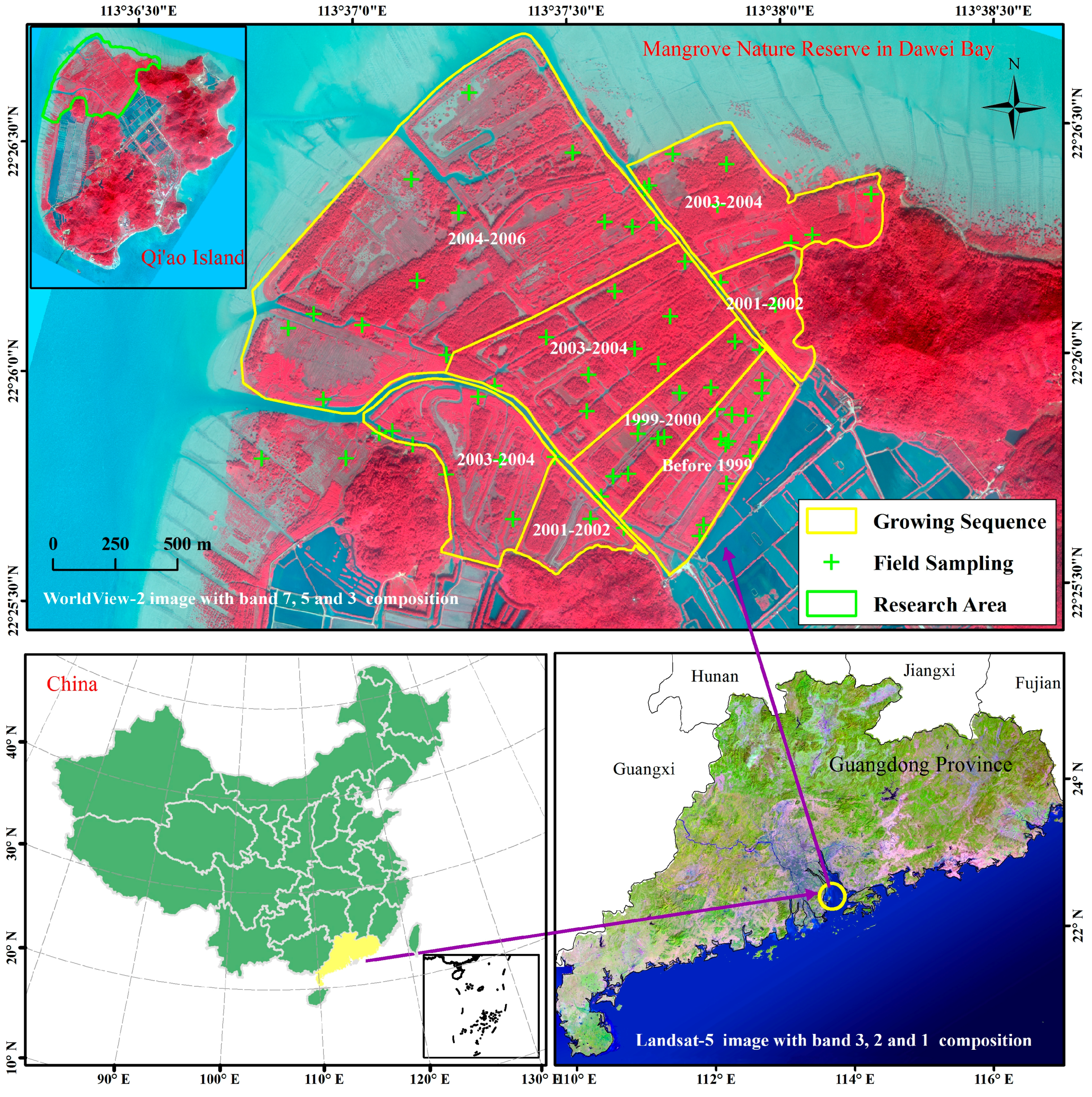
2.1. Study Area
2.2. Measurement of LAI
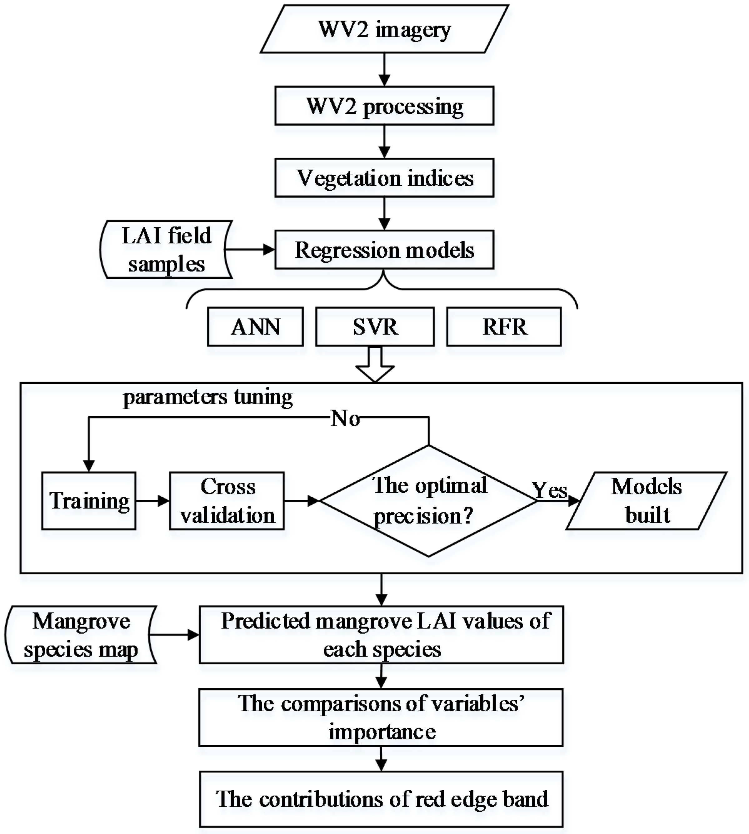
2.3. Workflow for the Analyses
2.4. Remotely Sensed Data and Processing
2.5. Mangrove Classification Based on WorldView-2 Imagery
2.6. Calculation of VIs from WorldView-2 Imagery
2.7. LAI Inversion Modeling and Accuracy Assessment
2.7.1. Artificial Neural Network Regression (ANNR)
2.7.2. Support Vector Regression (SVR)
2.7.3. Random Forest Regression (RFR)
2.7.4. Accuracy Assessment
3. Results
3.1. Mangrove Classification
3.2. Model Results and Accuracy Assessment
3.3. Variable Importance
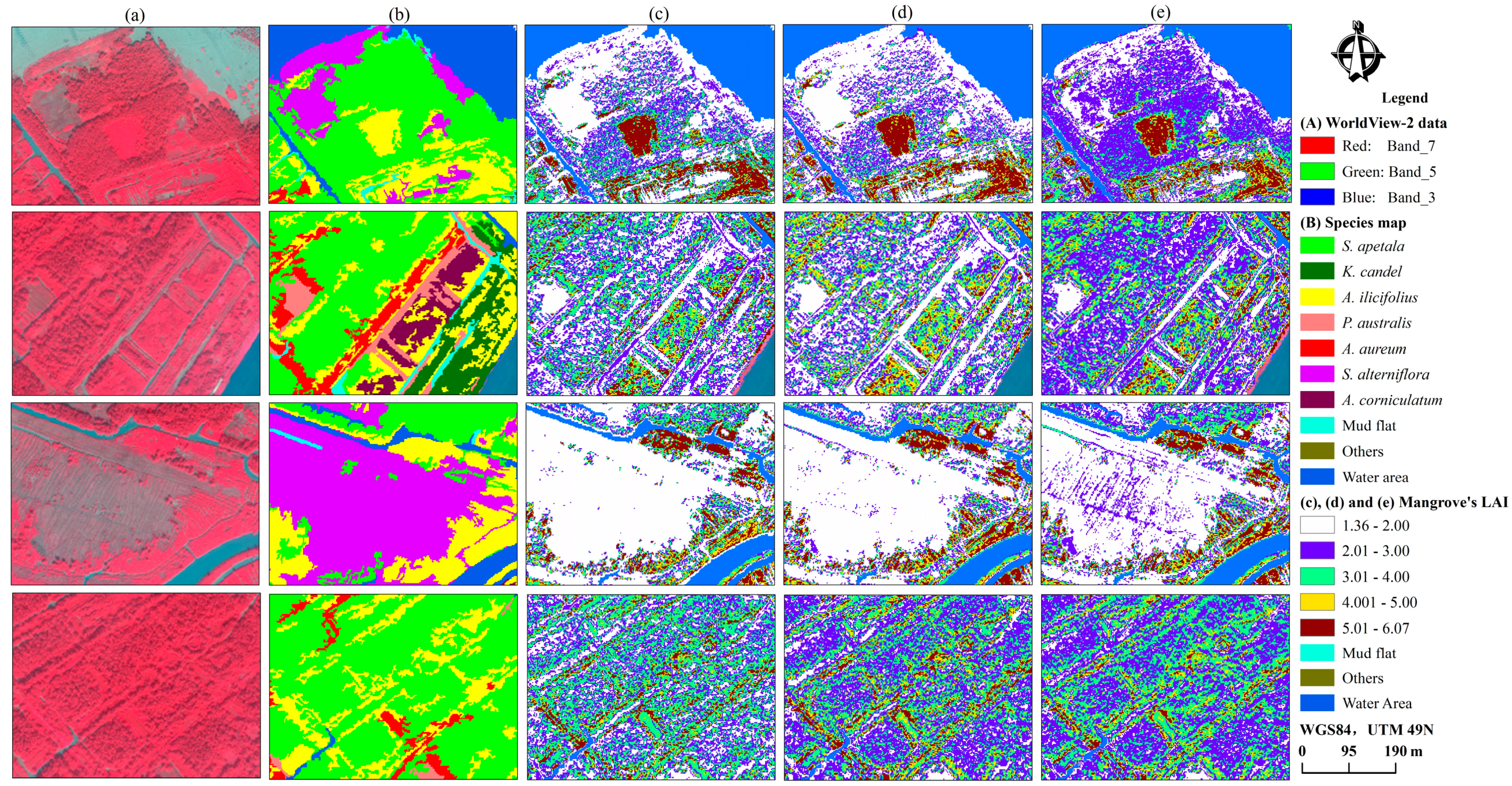
3.4. Spatial Distribution of Mangrove Vegetation LAI
4. Discussion
4.1. Spatial Distribution Characteristics of LAI for Mangrove Species
4.2. Overall Performance of the LAI Model
4.3. Effect of the Red-Edge Band on LAI Estimation
5. Conclusions
Acknowledgments
Author Contributions
Conflicts of Interest
References
- Alongi, D.M. Carbon sequestration in mangrove forests. Carbon Manag. 2012, 3, 313–322. [Google Scholar] [CrossRef]
- Diele, K.; Koch, V.; Saint-Paul, U. Population structure, catch composition and cpue of the artisanally harvested mangrove crab ucides cordatus (ocypodidae) in the caeté estuary, north brazil: Indications for overfishing? Aquat. Living Resour. 2005, 18, 169–178. [Google Scholar] [CrossRef]
- Das, S.; Vincent, J.R. Mangroves protected villages and reduced death toll during indian super cyclone. Proc. Natl. Acad. Sci. USA 2009, 106, 7357–7360. [Google Scholar] [CrossRef] [PubMed]
- Zhang, K.Q. Identification of gaps in mangrove forests with airborne lidar. Remote Sens. Environ. 2008, 112, 2309–2325. [Google Scholar] [CrossRef]
- Nagelkerken, I.; Blaber, S.J.M.; Bouillon, S.; Green, P.; Haywood, M.; Kirton, L.G.; Meynecke, J.O.; Pawlik, J.; Penrose, H.M.; Sasekumar, A.; et al. The habitat function of mangroves for terrestrial and marine fauna: A review. Aquat. Bot. 2008, 89, 155–185. [Google Scholar] [CrossRef]
- Liu, X.P.; Li, X.; Chen, Y.M.; Tan, Z.Z.; Li, S.Y.; Ai, B. A new landscape index for quantifying urban expansion using multi-temporal remotely sensed data. Landsc. Ecol. 2010, 25, 671–682. [Google Scholar] [CrossRef]
- Ross, M.S.; Sah, J.P.; Meeder, J.F.; Ruiz, P.L.; Telesnicki, G. Compositional effects of sea-level rise in a patchy landscape: The dynamics of tree islands in the southeastern coastal everglades. Wetlands 2014, 34, S91–S100. [Google Scholar] [CrossRef]
- Giri, C.; Ochieng, E.; Tieszen, L.L.; Zhu, Z.; Singh, A.; Loveland, T.; Masek, J.; Duke, N. Status and distribution of mangrove forests of the world using earth observation satellite data. Glob. Ecol. Biogeogr. 2011, 20, 154–159. [Google Scholar] [CrossRef]
- Liu, K.; Li, X.; Shi, X.; Wang, S.G. Monitoring mangrove forest changes using remote sensing and gis data with decision-tree learning. Wetlands 2008, 28, 336–346. [Google Scholar] [CrossRef]
- Ren, H.; Jian, S.G.; Lu, H.F.; Zhang, Q.M.; Shen, W.J.; Han, W.D.; Yin, Z.Y.; Guo, Q.F. Restoration of mangrove plantations and colonisation by native species in leizhou bay, south china. Ecol. Res. 2008, 23, 401–407. [Google Scholar] [CrossRef]
- Liu, K.; Liu, L.; Liu, H.X.; Li, X.; Wang, S.G. Exploring the effects of biophysical parameters on the spatial pattern of rare cold damage to mangrove forests. Remote Sens. Environ. 2014, 150, 20–33. [Google Scholar] [CrossRef]
- Flores-de-Santiago, F.; Kovacs, J.M.; Flores-Verdugo, F. The influence of seasonality in estimating mangrove leaf chlorophyll-a content from hyperspectral data. Wetl. Ecol. Manag. 2013, 21, 193–207. [Google Scholar] [CrossRef]
- Laurent, V.C.E.; Schaepman, M.E.; Verhoef, W.; Weyermann, J.; Chavez, R.O. Bayesian object-based estimation of lai and chlorophyll from a simulated sentinel-2 top-of-atmosphere radiance image. Remote Sens. Environ. 2014, 140, 318–329. [Google Scholar] [CrossRef]
- Liu, Y.; Liu, R.G.; Chen, J.M. Retrospective retrieval of long-term consistent global leaf area index (1981–2011) from combined avhrr and modis data. J. Geophys. Res. Biogeosci. 2012, 117, 1–14. [Google Scholar] [CrossRef]
- Canisius, F.; Fernandes, R.; Chen, J. Comparison and evaluation of medium resolution imaging spectrometer leaf area index products across a range of land use. Remote Sens. Environ. 2010, 114, 950–960. [Google Scholar] [CrossRef]
- Kovacs, J.M.; King, J.M.; Flores de Santiago, F.; Flores-Verdugo, F. Evaluating the condition of a mangrove forest of the mexican pacific based on an estimated leaf area index mapping approach. Environ. Monit. Assess. 2009, 157, 137–149. [Google Scholar] [CrossRef] [PubMed]
- Carlson, T.N.; Ripley, D.A. On the relation between ndvi, fractional vegetation cover, and leaf area index. Remote Sens. Environ. 1997, 62, 241–252. [Google Scholar] [CrossRef]
- Wang, L.; Sousa, W.P.; Gong, P.; Biging, G.S. Comparison of ikonos and quickbird images for mapping mangrove species on the caribbean coast of panama. Remote Sens. Environ. 2004, 91, 432–440. [Google Scholar] [CrossRef]
- Ozdemir, I.; Karnieli, A. Predicting forest structural parameters using the image texture derived from worldview-2 multispectral imagery in a dryland forest, israel. Int. J. Appl. Earth Obs. Geoinf. 2011, 13, 701–710. [Google Scholar] [CrossRef]
- Karlson, M.; Ostwald, M.; Reese, H.; Bazié, H.R.; Tankoano, B. Assessing the potential of multi-seasonal worldview-2 imagery for mapping west african agroforestry tree species. Int. J. Appl. Earth Obs. Geoinf. 2016, 50, 80–88. [Google Scholar] [CrossRef]
- Adjorlolo, C.; Mutanga, O.; Cho, M.A. Estimation of canopy nitrogen concentration across c3 and c4 grasslands using worldview-2 multispectral data. IEEE J. Sel. Top. Appl. Earth Obs. Remote Sens. 2014, 7, 4385–4392. [Google Scholar] [CrossRef]
- Ramoelo, A.; Cho, M.A.; Mathieu, R.; Madonsela, S.; Van De Kerchove, R.; Kaszta, Z.; Wolff, E. Monitoring grass nutrients and biomass as indicators of rangeland quality and quantity using random forest modelling and worldview-2 data. Int. J. Appl. Earth Obs. Geoinf. 2015, 43, 43–54. [Google Scholar] [CrossRef]
- Deng, S.Q.; Katoh, M.; Guan, Q.W.; Yin, N.; Li, M.Y. Interpretation of forest resources at the individual tree level at purple mountain, Nanjing city, China, using worldview-2 imagery by combining gps, rs and gis technologies. Remote Sens. 2014, 6, 87–110. [Google Scholar] [CrossRef]
- Adi, N.S.; Phinn, S.; Roelfsema, C.; Samper-Villarreal, J. Integrating field and remote sensing approaches for mapping seagrass leaf area index. In Proceedings of the 34th Asian Conference on Remote Sensing 2013 (ACRS 2013), Bali, Indonesia, 20–24 October 2013; Asian Association on Remote Sensing: Bali, Indonesia, 2013; pp. 3273–3280. [Google Scholar]
- Kamal, M.; Phinn, S.; Johansen, K. Assessment of multi-resolution image data for mangrove leaf area index mapping. Remote Sens. Environ. 2016, 176, 242–254. [Google Scholar] [CrossRef]
- Pu, R.L.; Cheng, J. Mapping forest leaf area index using reflectance and textural information derived from worldview-2 imagery in a mixed natural forest area in Florida, US. Int. J. Appl. Earth Obs. Geoinf. 2015, 42, 11–23. [Google Scholar] [CrossRef]
- Pope, G.; Treitz, P. Leaf area index (lai) estimation in boreal mixedwood forest of ontario, canada using light detection and ranging (lidar) and worldview-2 imagery. Remote Sens. 2013, 5, 5040–5063. [Google Scholar] [CrossRef]
- Kovacs, J.M.; Wang, J.; Flores-Verdugo, F. Mapping mangrove leaf area index at the species level using ikonos and lai-2000 sensors for the agua brava lagoon, mexican pacific. Estuar. Coast. Shelf Sci. 2005, 62, 377–384. [Google Scholar] [CrossRef]
- Vaiphasa, C.; Ongsomwang, S.; Vaiphasa, T.; Skidmore, A.K. Tropical mangrove species discrimination using hyperspectral data: A laboratory study. Estuar. Coast. Shelf Sci. 2005, 65, 371–379. [Google Scholar] [CrossRef]
- Kovacs, J.M.; Lu, X.X.; Flores-Verdugo, F.; Zhang, C.; de Santiago, F.F.; Jiao, X. Applications of alos palsar for monitoring biophysical parameters of a degraded black mangrove (avicennia germinans) forest. ISPRS J. Photogramm. Remote Sens. 2013, 82, 102–111. [Google Scholar] [CrossRef]
- Kovacs, J.M.; de Santiago, F.F.; Bastien, J.; Lafrance, P. An assessment of mangroves in guinea, west africa, using a field and remote sensing based approach. Wetlands 2010, 30, 773–782. [Google Scholar] [CrossRef]
- Kovacs, J.M.; Vandenberg, C.V.; Wang, J.; Flores-Verdugo, F. The use of multipolarized spaceborne sar backscatter for monitoring the health of a degraded mangrove forest. J. Coast. Res. 2008, 24, 248–254. [Google Scholar] [CrossRef]
- Kovacs, J.M.; Vandenberg, C.V.; Flores-Verdugo, F. Assessing fine beam radarsat-1 backscatter from a white mangrove (laguncularia racemosa (gaertner)) canopy. Wetl. Ecol. Manag. 2006, 14, 401–408. [Google Scholar] [CrossRef]
- Wong, F.K.K.; Fung, T. Combining hyperspectral and radar imagery for mangrove leaf area index modeling. Photogramm. Eng. Remote Sens. 2013, 79, 479–490. [Google Scholar] [CrossRef]
- Horler, D.; Dockray, M.; Barber, J. The red edge of plant leaf reflectance. Int. J. Remote Sens. 1983, 4, 273–288. [Google Scholar] [CrossRef]
- Mutanga, O.; Skidmore, A.K. Integrating imaging spectroscopy and neural networks to map grass quality in the kruger national park, south africa. Remote Sens. Environ. 2004, 90, 104–115. [Google Scholar] [CrossRef]
- Van Deventer, H.; Cho, M.A.; Mutanga, O.; Ramoelo, A. Capability of models to predict leaf n and p across four seasons for six sub-tropical forest evergreen trees. ISPRS J. Photogramm. Remote Sens. 2015, 101, 209–220. [Google Scholar] [CrossRef]
- Cho, M.A.; Ramoelo, A.; Debba, P.; Mutanga, O.; Mathieu, R.; van Deventer, H.; Ndlovu, N. Assessing the effects of subtropical forest fragmentation on leaf nitrogen distribution using remote sensing data. Landsc. Ecol. 2013, 28, 1479–1491. [Google Scholar] [CrossRef]
- Mutanga, O.; Adam, E.; Cho, M.A. High density biomass estimation for wetland vegetation using worldview-2 imagery and random forest regression algorithm. Int. J. Appl. Earth Obs. Geoinf. 2012, 18, 399–406. [Google Scholar] [CrossRef]
- Siegmann, B.; Jarmer, T. Comparison of different regression models and validation techniques for the assessment of wheat leaf area index from hyperspectral data. Int. J. Remote Sens. 2015, 36, 4519–4534. [Google Scholar] [CrossRef]
- Houborg, R.; Boegh, E. Mapping leaf chlorophyll and leaf area index using inverse and forward canopy reflectance modeling and spot reflectance data. Remote Sens. Environ. 2008, 112, 186–202. [Google Scholar] [CrossRef]
- Gonzalez-Sanpedro, M.C.; Le Toan, T.; Moreno, J.; Kergoat, L.; Rubio, E. Seasonal variations of leaf area index of agricultural fields retrieved from landsat data. Remote Sens. Environ. 2008, 112, 810–824. [Google Scholar] [CrossRef]
- Schlerf, M.; Atzberger, C. Inversion of a forest reflectance model to estimate structural canopy variables from hyperspectral remote sensing data. Remote Sens. Environ. 2006, 100, 281–294. [Google Scholar] [CrossRef]
- Breiman, L. Random forests. Mach. Learn. 2001, 45, 5–32. [Google Scholar] [CrossRef]
- Prasad, R.; Pandey, A.; Singh, K.P.; Singh, V.P.; Mishra, R.K.; Singh, D. Retrieval of spinach crop parameters by microwave remote sensing with back propagation artificial neural networks: A comparison of different transfer functions. Adv. Space Res. 2012, 50, 363–370. [Google Scholar] [CrossRef]
- Walthall, C.; Dulaney, W.; Anderson, M.; Norman, J.; Fang, H.L.; Liang, S.L. A comparison of empirical and neural network approaches for estimating corn and soybean leaf area index from landsat etm+ imagery. Remote Sens. Environ. 2004, 92, 465–474. [Google Scholar] [CrossRef]
- Feilhauer, H.; Asner, G.P.; Martin, R.E. Multi-method ensemble selection of spectral bands related to leaf biochemistry. Remote Sens. Environ. 2015, 164, 57–65. [Google Scholar] [CrossRef]
- Jachowski, N.R.A.; Quak, M.S.Y.; Friess, D.A.; Duangnamon, D.; Webb, E.L.; Ziegler, A.D. Mangrove biomass estimation in southwest thailand using machine learning. Appl. Geogr. 2013, 45, 311–321. [Google Scholar] [CrossRef]
- Tang, H.; Liu, K.; Zhu, Y.; Wang, S.; Liu, L.; Song, S. Mangrove community classification based on worldview-2 image and svm method. Acta Sci. Nat. Univ. Sunyatseni 2015, 54, 102–111. [Google Scholar]
- Zhu, Y.H.; Liu, K.; Liu, L.; Wang, S.G.; Liu, H.X. Retrieval of mangrove aboveground biomass at the individual species level with worldview-2 images. Remote Sens. 2015, 7, 12192–12214. [Google Scholar] [CrossRef]
- Wu, Z.J.; Zhou, H.Y.; Ren, D.Z.; Gao, H.; Li, J.T. Processes controlling the seasonal and spatial variations in sulfate profiles in the pore water of the sediments surrounding Qi’ao Island, Pearl River Estuary, Southern China. Cont. Shelf Res. 2015, 98, 26–35. [Google Scholar] [CrossRef]
- Li, X.; Yeh, A.G.O.; Wang, S.; Liu, K.; Liu, X.; Qian, J.; Chen, X. Regression and analytical models for estimating mangrove wetland biomass in south china using radarsat images. Int. J. Remote Sens. 2007, 28, 5567–5582. [Google Scholar] [CrossRef]
- Piayda, A.; Dubbert, M.; Werner, C.; Vaz Correia, A.; Pereira, J.S.; Cuntz, M. Influence of woody tissue and leaf clumping on vertically resolved leaf area index and angular gap probability estimates. For. Ecol. Manag. 2015, 340, 103–113. [Google Scholar] [CrossRef]
- Kovacs, J.M.; Flores-Verdugo, F.; Wang, J.F.; Aspden, L.P. Estimating leaf area index of a degraded mangrove forest using high spatial resolution satellite data. Aquat. Bot. 2004, 80, 13–22. [Google Scholar] [CrossRef]
- Chen, J.M.; Cihlar, J. Retrieving leaf area index of boreal conifer forests using landsat tm images. Remote Sens. Environ. 1996, 55, 153–162. [Google Scholar] [CrossRef]
- Rumelhart, D.E.; McClelland, J.L.; PDP Research Group. Parallel Distributed Processing; The MIT Press: Cambridge, MA, USA, 1986; Volume 1–2. [Google Scholar]
- Cortes, C.; Vapnik, V. Support-vector networks. Mach. Learn. 1995, 20, 273–297. [Google Scholar] [CrossRef]
- Wieland, M.; Pittore, M. Performance evaluation of machine learning algorithms for urban pattern recognition from multi-spectral satellite images. Remote Sens. 2014, 6, 2912–2939. [Google Scholar] [CrossRef]
- Ruizluna, A.; Escobar, A.C.; Berlangarobles, C. Assessing distribution patterns, extent, and current condition of northwest mexico mangroves. Wetlands 2010, 30, 717–723. [Google Scholar] [CrossRef]
- Pu, R.L.; Landry, S. A comparative analysis of high spatial resolution ikonos and worldview-2 imagery for mapping urban tree species. Remote Sens. Environ. 2012, 124, 516–533. [Google Scholar] [CrossRef]
- Haboudane, D.; Miller, J.R.; Tremblay, N.; Zarco-Tejada, P.J.; Dextraze, L. Integrated narrow-band vegetation indices for prediction of crop chlorophyll content for application to precision agriculture. Remote Sens. Environ. 2002, 81, 416–426. [Google Scholar] [CrossRef]
- Pena-Barragan, J.M.; Ngugi, M.K.; Plant, R.E.; Six, J. Object-based crop identification using multiple vegetation indices, textural features and crop phenology. Remote Sens. Environ. 2011, 115, 1301–1316. [Google Scholar] [CrossRef]
- Eckert, S. Improved forest biomass and carbon estimations using texture measures from worldview-2 satellite data. Remote Sens. 2012, 4, 810–829. [Google Scholar] [CrossRef]
- Anastasladis, A.D.; Magoulas, G.D.; Vrahatis, M.N. New globally convergent training scheme based on the resilient propagation algorithm. Neurocomputing 2005, 64, 253–270. [Google Scholar] [CrossRef]
- Chang, C.C.; Lin, C.J. Libsvm: A library for support vector machines. ACM Trans. Intell. Syst. Technol. 2011, 2, 1–27. [Google Scholar] [CrossRef]
- Liaw, A.; Wiener, M. Classification and regression by randomforest. R News 2002, 2, 18–22. [Google Scholar]
- Fassnacht, F.E.; Hartig, F.; Latifi, H.; Berger, C.; Hernandez, J.; Corvalan, P.; Koch, B. Importance of sample size, data type and prediction method for remote sensing-based estimations of aboveground forest biomass. Remote Sens. Environ. 2014, 154, 102–114. [Google Scholar] [CrossRef]
- Axelsson, C.; Skidmore, A.K.; Schlerf, M.; Fauzi, A.; Verhoef, W. Hyperspectral analysis of mangrove foliar chemistry using plsr and support vector regression. Int. J. Remote Sens. 2013, 34, 1724–1743. [Google Scholar] [CrossRef]
- Wang, L.; Silván-Cárdenas, J.L.; Sousa, W.P. Neural network classification of mangrove species from multiseasonal ikonos imagery. Photogramm. Eng. Remote Sens. 2008, 74, 921–927. [Google Scholar] [CrossRef]
- Liu, X.; Li, X.; Shi, X.; Wu, S.; Liu, T. Simulating complex urban development using kernel-based non-linear cellular automata. Ecol. Model. 2008, 211, 169–181. [Google Scholar] [CrossRef]
- Rumelhart, D.E.; Hinton, G.E.; Williams, R.J. Learning representations by back-propagating errors. Nature 1986, 323, 533–536. [Google Scholar] [CrossRef]
- Olden, J.D.; Joy, M.K.; Death, R.G. An accurate comparison of methods for quantifying variable importance in artificial neural networks using simulated data. Ecol. Model. 2004, 178, 389–397. [Google Scholar] [CrossRef]
- Garson, G.D. Interpreting Neural-Network Connection Weights; Miller Freeman, Inc.: San Francisco, CA, USA, 1991; pp. 46–51. [Google Scholar]
- Mountrakis, G.; Im, J.; Ogole, C. Support vector machines in remote sensing: A review. ISPRS J. Photogramm. Remote Sens. 2011, 66, 247–259. [Google Scholar] [CrossRef]
- Üstün, B.; Melssen, W.J.; Buydens, L.M.C. Visualisation and interpretation of support vector regression models. Anal. Chim. Acta 2007, 595, 299–309. [Google Scholar] [CrossRef] [PubMed]
- Pal, M. Random forest classifier for remote sensing classification. Int. J. Remote Sens. 2005, 26, 217–222. [Google Scholar] [CrossRef]
- Zhang, J.; Huang, S.; Hogg, E.H.; Lieffers, V.; Qin, Y.; He, F. Estimating spatial variation in alberta forest biomass from a combination of forest inventory and remote sensing data. Biogeosciences 2014, 11, 2793–2808. [Google Scholar] [CrossRef] [Green Version]
- Cutler, D.R.; Edwards, T.C., Jr.; Beard, K.H.; Cutler, A.; Hess, K.T.; Gibson, J.; Lawler, J.J. Random forests for classification in ecology. Ecology 2007, 88, 2783–2792. [Google Scholar] [CrossRef] [PubMed]
- Cracknell, M.J.; Reading, A.M. Geological mapping using remote sensing data: A comparison of five machine learning algorithms, their response to variations in the spatial distribution of training data and the use of explicit spatial information. Comput. Geosci. 2014, 63, 22–33. [Google Scholar] [CrossRef]
- Heenkenda, M.K.; Joyce, K.E.; Maier, S.W.; de Bruin, S. Quantifying mangrove chlorophyll from high spatial resolution imagery. ISPRS J. Photogramm. Remote Sens. 2015, 108, 234–244. [Google Scholar] [CrossRef]
- Darvishzadeh, R.; Atzberger, C.; Skidmore, A.K.; Abkar, A.A. Leaf area index derivation from hyperspectral vegetation indicesand the red edge position. Int. J. Remote Sens. 2009, 30, 6199–6218. [Google Scholar] [CrossRef]
- Broge, N.H.; Leblanc, E. Comparing prediction power and stability of broadband and hyperspectral vegetation indices for estimation of green leaf area index and canopy chlorophyll density. Remote Sens. Environ. 2001, 76, 156–172. [Google Scholar] [CrossRef]
- Adam, E.; Mutanga, O.; Abdel-Rahman, E.M.; Ismail, R. Estimating standing biomass in papyrus (Cyperus papyrus L.) swamp: Exploratory of in situ hyperspectral indices and random forest regression. Int. J. Remote Sens. 2014, 35, 693–714. [Google Scholar] [CrossRef]
- Malahlela, O.; Cho, M.A.; Mutanga, O. Mapping canopy gaps in an indigenous subtropical coastal forest using high-resolution worldview-2 data. Int. J. Remote Sens. 2014, 35, 6397–6417. [Google Scholar] [CrossRef]
- Dube, T.; Mutanga, O.; Elhadi, A.; Ismail, R. Intra-and-inter species biomass prediction in a plantation forest: Testing the utility of high spatial resolution spaceborne multispectral rapideye sensor and advanced machine learning algorithms. Sensors 2014, 14, 15348–15370. [Google Scholar] [CrossRef] [PubMed]


| Types of Bands | Wavebands | Spectral Band Edges | Spatial Resolution | |
|---|---|---|---|---|
| The traditional bands | B2 | blue band | 450 nm to 510 nm | 2 m |
| B3 | green band | 510 nm to 580 nm | ||
| B5 | red band | 630 nm to 690 nm | ||
| B7 | near-infrared-1 band | 770 nm to 895 nm | ||
| The new bands | B1 | coastal band | 400 nm to 450 nm | |
| B4 | yellow band | 585 nm to 625 nm | ||
| B6 | red-edge band | 705 nm to 745 nm | ||
| B8 | near-infrared-2 band | 860 nm to 1040 nm | ||
| The panchromatic band | -- | -- | -- | 0.5 m |
| Bands | VI | Commonly Related to | Ref. |
|---|---|---|---|
| Red-edge band (B6) | RedEdge Normalized Difference Vegetation Index | canopy foliage content, gap fraction, and senescence | [60] |
| RedEdge Simple Ratio Index | Chlorophyll concentration and moisture content | ||
| Modified RedEdge Simple Ratio Index | precision agriculture, forest monitoring, and vegetation stress detection | ||
| RedEdge Normalized Difference Vegetation Index | Vegetation status, canopy structure | ||
| RedEdge Simple Ratio Index | Vegetation status, canopy structure | ||
| Modified Chlorophyll Absorption in Reflectance Index | relative abundance of chlorophyll, leaf pigments and vegetation status | [61] | |
| Transformed Chlorophyll Absorption in Reflectance Index | relative abundance of chlorophyll, leaf pigments and vegetation status | ||
| Triangular Vegetation Index | Leaf pigments, vegetation status and green LAI, | ||
| eeNear-infrared-1 band (B7) | Normalized Difference Vegetation Index | Vegetation status, canopy structure | [62] |
| Simple Ratio Index | Vegetation status, canopy structure | ||
| Green Normalized Difference Vegetation Index | Leaf pigments, vegetation greenish | ||
| Modified Simple Ratio | Vegetation status, canopy structure | ||
| Modified Chlorophyll Absorption in Reflectance Index | Leaf pigments, vegetation status | ||
| Transformed Chlorophyll Absorption in Reflectance Index | Leaf pigments, vegetation status | ||
| Optimized soil-Adjusted Vegetation Index | soil variation in low vegetation cover, | [61] | |
| Environmental Vegetation Index | the vegetation signal in LAI regions | [63] | |
| Near-infrared-2 band (B8) | Normalized Difference Vegetation Index | Vegetation status, canopy structure | [60] |
| Simple Ratio Index | Vegetation status, canopy structure | ||
| Normalized Difference Vegetation Index | Vegetation status, canopy structure | ||
| Simple Ratio Index | Vegetation status, canopy structure |
| Classified Data | Reference Data | ||||||||
|---|---|---|---|---|---|---|---|---|---|
| SA | AI | SAP | PA | AC | KC | AA | Mudflat | Total | |
| SA | 96 | 9 | 4 | 1 | 0 | 0 | 5 | 13 | 128 |
| AI | 0 | 155 | 31 | 0 | 16 | 1 | 2 | 0 | 205 |
| SAP | 0 | 3 | 367 | 3 | 0 | 0 | 4 | 11 | 388 |
| PA | 0 | 0 | 3 | 26 | 0 | 0 | 0 | 7 | 36 |
| AC | 0 | 0 | 0 | 0 | 31 | 0 | 0 | 0 | 31 |
| KC | 0 | 0 | 0 | 5 | 0 | 59 | 0 | 0 | 64 |
| AA | 0 | 12 | 4 | 12 | 0 | 0 | 28 | 1 | 57 |
| Mudflat | 0 | 0 | 6 | 1 | 0 | 2 | 0 | 70 | 79 |
| Total | 96 | 179 | 179 | 48 | 47 | 62 | 39 | 102 | - |
| Over accuracy: 84.2%; Kappa: 0.794 | |||||||||
| Models | The Tuning Parameters | Setting Range | Interval | The Optimal Value |
|---|---|---|---|---|
| ANNR | HLN | 2–20 | 2 | 12, 7 |
| NI | 500–15,000 | 500 | 7000 | |
| SVR | C | 2−10–210 | Multiply by 2 | 2 |
| γ | 2−10–210 | Multiply by 2 | 0.03125 | |
| RFR | ntree | 100–5000 | 100 | 300 |
| mtry | 2–20 | 2 | 12 |
| Parameters | Models | RMSEs | Average RMSE | Average RMSEr | ||||
|---|---|---|---|---|---|---|---|---|
| All of VIs | ANNR | 0.39 | 0.51 | 0.52 | 0.48 | 0.57 | 0.49 | 16.04% |
| SVR | 0.42 | 0.45 | 0.56 | 0.48 | 0.64 | 0.51 | 16.56% | |
| RFR | 0.41 | 0.35 | 0.55 | 0.45 | 0.48 | 0.45 | 14.55% | |
| Removing VIs Derived from red-edge band | ANNR | 0.65 | 0.58 | 0.69 | 0.41 | 0.72 | 0.61 | 19.83% |
| SVR | 0.54 | 0.49 | 0.48 | 0.73 | 0.72 | 0.59 | 19.26% | |
| RFR | 0.63 | 0.72 | 0.49 | 0.67 | 0.42 | 0.58 | 19.02% | |
| VIs Derived from red-edge band | ANNR | 0.53 | 0.58 | 0.67 | 0.75 | 0.50 | 0.60 | 19.57% |
| SVR | 0.66 | 0.64 | 0.62 | 0.60 | 0.63 | 0.63 | 20.47% | |
| RFR | 0.64 | 0.65 | 0.73 | 0.44 | 0.42 | 0.58 | 18.71% | |
| VIs Derived from near-infrared-1 | ANNR | 0.51 | 0.51 | 0.95 | 0.71 | 0.71 | 0.68 | 22.01% |
| SVR | 0.64 | 0.77 | 0.85 | 0.42 | 0.71 | 0.68 | 21.97% | |
| RFR | 0.76 | 0.66 | 0.57 | 0.73 | 0.51 | 0.65 | 20.98% | |
| VIs Derived from near-infrared-2 | ANNR | 0.80 | 0.73 | 0.70 | 0.98 | 0.53 | 0.75 | 24.31% |
| SVR | 0.79 | 0.89 | 0.84 | 0.54 | 0.86 | 0.78 | 25.38% | |
| RFR | 0.83 | 0.70 | 0.79 | 0.64 | 0.64 | 0.72 | 23.41% | |
| VIs | ANNR | SVR | RFR | |||
|---|---|---|---|---|---|---|
| Variable Importance | Ranks | Variable Importance | Ranks | Variable Importance | Ranks | |
| RE-NDVI65 | 0.97 | 7 | 2.22 | 7 | 2.7 | 2 |
| RE-SR65 | 2.00 | 2 | 2.44 | 1 | 3.83 | 1 |
| MRE-SR651 | 0.03 | 19 | 2.25 | 5 | 0.69 | 9 |
| RE-NDVI61 | 0.08 | 18 | 2.02 | 12 | 0.05 | 19 |
| RE-SR61 | 1.32 | 5 | 2.00 | 15 | 0.17 | 17 |
| MCARI653 | 2.14 | 1 | 2.41 | 2 | 2.59 | 3 |
| TCARI653 | 0.09 | 17 | 1.21 | 20 | 0.04 | 20 |
| TVI653 | 0.66 | 9 | 2.15 | 9 | 0.64 | 10 |
| NDVI75 | 0.41 | 10 | 2.03 | 10 | 1.02 | 5 |
| SRI75 | 0.26 | 12 | 2.26 | 4 | 0.97 | 6 |
| GNDVI73 | 1.09 | 6 | 2.01 | 13 | 0.43 | 13 |
| MSR75 | 0.18 | 15 | 2.28 | 3 | 1.06 | 4 |
| MCARI753 | 0.86 | 8 | 2.21 | 8 | 0.38 | 15 |
| TCARI753 | 0.37 | 11 | 2.24 | 6 | 0.06 | 18 |
| OSAVI75 | 0.02 | 20 | 2.03 | 11 | 0.29 | 16 |
| EVI752 | 0.21 | 14 | 2.00 | 14 | 0.54 | 12 |
| NDVI84 | 0.26 | 13 | 1.51 | 19 | 0.42 | 14 |
| NDVI85 | 1.75 | 3 | 1.71 | 18 | 0.8 | 8 |
| SRI84 | 1.34 | 4 | 1.77 | 17 | 0.59 | 11 |
| SRI85 | 0.13 | 16 | 1.98 | 16 | 0.89 | 7 |
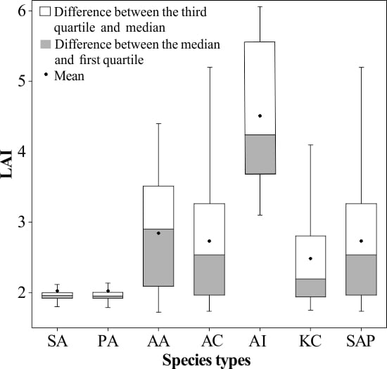
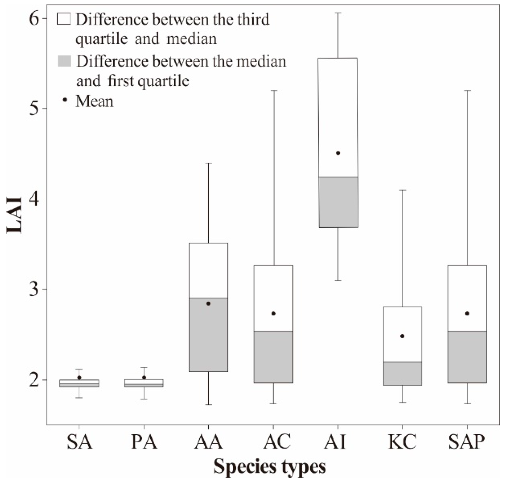
| Community Types | Species | LAI Range | Mean LAI | SD |
|---|---|---|---|---|
| Herbaceous | S. alterniflora | 1.70–2.44 | 2.02 | 0.30 |
| P. australis | 1.73–2.42 | 2.02 | 0.27 | |
| A. aureum | 1.72–4.40 | 2.84 | 0.73 | |
| Shrub | A. corniculatum | 1.73–5.55 | 2.73 | 0.86 |
| A. ilicifolius | 3.10–6.06 | 4.51 | 0.92 | |
| Tree | K. candel | 1.75–4.38 | 2.48 | 0.73 |
| S. apetala | 1.74–5.35 | 2.73 | 0.86 |
© 2017 by the authors. Licensee MDPI, Basel, Switzerland. This article is an open access article distributed under the terms and conditions of the Creative Commons Attribution (CC BY) license (http://creativecommons.org/licenses/by/4.0/).
Share and Cite
Zhu, Y.; Liu, K.; Liu, L.; Myint, S.W.; Wang, S.; Liu, H.; He, Z. Exploring the Potential of WorldView-2 Red-Edge Band-Based Vegetation Indices for Estimation of Mangrove Leaf Area Index with Machine Learning Algorithms. Remote Sens. 2017, 9, 1060. https://doi.org/10.3390/rs9101060
Zhu Y, Liu K, Liu L, Myint SW, Wang S, Liu H, He Z. Exploring the Potential of WorldView-2 Red-Edge Band-Based Vegetation Indices for Estimation of Mangrove Leaf Area Index with Machine Learning Algorithms. Remote Sensing. 2017; 9(10):1060. https://doi.org/10.3390/rs9101060
Chicago/Turabian StyleZhu, Yuanhui, Kai Liu, Lin Liu, Soe W. Myint, Shugong Wang, Hongxing Liu, and Zhi He. 2017. "Exploring the Potential of WorldView-2 Red-Edge Band-Based Vegetation Indices for Estimation of Mangrove Leaf Area Index with Machine Learning Algorithms" Remote Sensing 9, no. 10: 1060. https://doi.org/10.3390/rs9101060
APA StyleZhu, Y., Liu, K., Liu, L., Myint, S. W., Wang, S., Liu, H., & He, Z. (2017). Exploring the Potential of WorldView-2 Red-Edge Band-Based Vegetation Indices for Estimation of Mangrove Leaf Area Index with Machine Learning Algorithms. Remote Sensing, 9(10), 1060. https://doi.org/10.3390/rs9101060