Feature-Based Nonlocal Polarimetric SAR Filtering

Abstract

Polarimetric synthetic aperture radar (PolSAR) images are inherently contaminated by multiplicative speckle noise, which complicates the image interpretation and image analyses. To reduce the speckle effect, several adaptive speckle filters have been developed based on the weighted average of the similarity measures commonly depending on the model or probability distribution, which are often affected by the distribution parameters and modeling texture components. In this paper, a novel filtering method introduces the coefficient of variance ($\mathrm{CV}$) and Pauli basis (PB) to measure the similarity, and the two features are combined with the framework of the nonlocal mean filtering. The $\mathrm{CV}$ is used to describe the complexity of various scenes and distinguish the scene heterogeneity; moreover, the Pauli basis is able to express the polarimetric information in PolSAR image processing. This proposed filtering combines the $\mathrm{CV}$ and Pauli basis to improve the estimation accuracy of the similarity weights. Then, the similarity of the features is deduced according to the test statistic. Subsequently, the filtering is proceeded by using the nonlocal weighted estimation. The performance of the proposed filter is tested with the simulated images and real PolSAR images, which are acquired by AIRSAR system and ESAR system. The qualitative and quantitative experiments indicate the validity of the proposed method by comparing with the widely-used despeckling methods.

1. Introduction

Synthetic aperture radar (SAR) explores the characterization of the Earth’s surface in the microwave range, which makes it possible to observe and retrieve data under all weather conditions and all times. Polarimetric SAR (PolSAR) systems further enrich the remote sensing information source, as the appearance of polarization diversity makes the remote sensing system more sensitive to the scattering properties of the imaged scene. However, the coherent imaging system is inherently contaminated by multiplicative speckle noise because of the coherent nature of the scattering. Therefore, the speckle filtering is always a fundamental step for PolSAR image processing.

So far, numerous kinds of speckle filter methods have been developed. The goal of speckle filtering is to suppress speckle while preserve spatial resolution and polarimetric information. Thus, the adaptive filtering methods are developing rapidly by using weighted averages of homogeneous pixels with similar scattering property. These filter algorithms have been widely applied to reduce speckle by using a weighted combination of the homogeneous sample and its mean. The refined Lee filter selected the similar pixels to reinforce homogeneity according to eight non-square windows as the templates [1,2]. Similarly, in the improved sigma filter, the two-sigma probability ranges were utilizes to select homogeneous pixels [3,4,5], and the intensity-driven adaptive-neighborhood (IDAN) was proposed by grouping pixels with similar statistical properties [6]. Furthermore, the bilateral filter calculates the weighted average based on the similarity between pixels in the local windows of the spatial and radiometric domains [7,8,9]. Generally, these filters are performed by the pixels close to the target, which implies these pixels that are similar in the local window. In reality, the notable differences between pixels exist in the heterogeneous regions, and the preservation of the image details is easily affected.

Recently, the nonlocal mean (NLM) filtering method applied to the PolSAR image computes the weights based on the patch similarity instead of the pixels [10]. Due to the structure information contained in patches, the patch similarity has been adapted to most state-of-the-art denoising techniques based on the test statistic [11], Bayesian framework [12], etc. Moreover, the nonlocal Lee (NL-Lee) filter combines the Lee filter with the framework of the NLM filter, and the homogeneity similarity is introduced to enhance the patch regularity assumption [13]. In [14], the NLM filter is involving in iterative steps and implemented in the form of maximum a posteriori (MAP). These nonlocal algorithms are mostly performed by applying the similarity measure of the matrix statistical estimation, and all the elements of the coherency matrix or covariance matrix are implemented in an identical manner. Therefore, the NLM filters depend on the model or probability distribution to measure the similarity, which are often affected by the distribution parameters and modeling texture components. Thus, few repeated structures may lead to poor results in the case of heterogeneous scenes with lots of details [15].

In the segmentation and classification methods, the extracted features can effectively measure the similarity between the pixels and the class center, and the different polarimetric signatures or features can distinguish the types of terrains from the different perspective [16,17,18,19]. Inspired by this idea, the similarity between the central pixel and each neighborhood pixel could be evaluated by the extracted feature.

Given the importance of the structural features for the speckle filters, the coefficient of variance ($\mathrm{CV}$) can reflect the complexity of different scenes, and it has been widely used in SAR and PolSAR image processing [20,21,22,23,24]. Moreover, this difference of the textural features can be quantitatively described by $\mathrm{CV}$, which could be used as the feature to measure the similarity. Electromagnetic scattering phenomena play a key role in the SAR image process. Moreover, the analysis of scattering mechanism for PolSAR image is the emphasis for information extraction and interpretation, etc. [25]. Scattering-model-based speckle filters have been proposed by combining the classification [26,27]. It is well known that the ground targets are much easier to be interpreted by the Pauli images. The Pauli basis (PB) corresponds to the polarization channel and can express most of the polarimetric information, and is usually used as the feature for polarimetric segmentation and classification [28,29]. Thus, the Pauli basis is chosen to better describe the scattering mechanisms.

The nonlocal mean filtering method has its advantages, and the pixels could be weighted according to the patch similarity. Therefore, the proposed filter introduces the features to the framework of the NLM filter to improve the estimation accuracy of the similarity weights. In this paper, the selected features are the $\mathrm{CV}$ and the Pauli basis (PB) based on the above analysis. Additionally, the similarity weights of the features are deduced according to the test statistic, and the filter is implemented by using weighted average of similar pixels. The combination of the extracted features can effectively enhance the discrimination of the target scattering mechanisms, and the test of the pixel similarity is more robust. The filtering performance is exhibited by using both simulated and real PolSAR data.

The remainder of this paper is organized as follows. The proposed filtering method is explained in detail in Section 2. The experimental results and different filtering methods for comparison analysis are listed in Section 3.The discussion of the results is presented in Section 4. The conclusions are given in Section 5.

2. Methodology

The proposed filtering method consists of three main parts: (1) the representation of the PolSAR data characteristics and Pauli decomposition; (2) the heterogeneity $\mathrm{CV}$ based on the polarimetric whitening filtering (PWF); (3) the nonlocal mean (NLM) filtering based on the $\mathrm{CV}$ and the Pauli basis. Figure 1 gives the flowchart of the proposed filtering algorithm. The details of each process are further described below.

2.1. Characteristics of PolSAR Data

The polarimetric characteristics of the ground objects are closely related to their geometric and dielectric properties. The characteristics can reflect the target surface roughness, symmetry, and other features information. PolSAR data offers efficient and reliable information required to extract biophysical and geophysical parameters about the Earth’s surface. The polarimetric information of the target can be expressed by the Sinclair scattering matrix [28]:

$$\mathit{S}=\left[\begin{array}{cc}{S}_{HH}& S_{HV}\\ S_{VH}& S_{VV}\end{array}\right]$$

(1)

where the elements $S_{HH}$ and $S_{VV}$ produce the power return in the copolarized channels, and the elements $S_{HV}$ and $S_{VH}$ produce the power return in the cross-polarized channels.

For a reciprocal target matrix, in the monostatic backscattering case, the Pauli basis vector $\mathit{k}$ for PolSAR can be expressed as:

$$\mathit{k}=\frac{1}{\sqrt{2}}{\left[S_{HH}+S_{VV},S_{HH}-S_{VV},2S_{HV}\right]}^t$$

(2)

where the superscript $t$ is the transpose operator. The $L$-look coherence matrix is given as $\mathrm{T}=\langle k{k}^{\ast t}\rangle =\frac{1}{L}{\sum }_{i=1}^{L}k\left(i\right)k{\left(i\right)}^{\ast t}$, where 〈·〉 is the ensemble average, $\ast t$ is the complex conjugate transpose, and $L$ is the number of looks.

In Pauli decomposition, the Sinclair scattering matrix is the complex sum of the Pauli matrices, with:

$$S=\left[\begin{array}{cc}{S}_{HH}& S_{HV}\\ S_{VH}& S_{VV}\end{array}\right]=\frac{a}{\sqrt{2}}\left[\begin{array}{cc}1& 0\\ 0& 1\end{array}\right]+\frac{b}{\sqrt{2}}\left[\begin{array}{cc}1& 0\\ 0& -1\end{array}\right]+\frac{c}{\sqrt{2}}\left[\begin{array}{cc}0& 1\\ 1& 0\end{array}\right]+\frac{d}{\sqrt{2}}\left[\begin{array}{cc}0& -j\\ j& 0\end{array}\right]$$

(3)

where $a$, $b$, $c$, and $d$ are all complex and are given by:

$$a=\frac{S_{HH}+S_{VV}}{\sqrt{2}},b=\frac{S_{HH}-S_{VV}}{\sqrt{2}},c=\frac{S_{HV}+S_{VV}}{\sqrt{2}},d=j\frac{S_{HV}-S_{VV}}{\sqrt{2}}$$

(4)

In the monostatic backscattering case, where $d=0$. It is noted that the Pauli basis is an incomplete representation of the polarimetric information of the scene due to only taking intensity into account. However, the expressions indicate that the Pauli spin matrix basis correspond to the matrix of the Pauli decomposition, and the polarimetric observations can be better applied. Thus, the Pauli basis is used to analyze the scattering mechanisms.

2.2. Scene Heterogeneity

The $\mathrm{CV}$ has been widely used to detect the scene heterogeneity, which was proposed to enhance the SAR filtering adaptively by Lopes et al. [20]. It is defined as the ratio between the standard deviation $\sigma$ and the mean $\mu$ in a local region as follows:

$$CV=\frac{\sigma }{\mu }$$

(5)

For polarimetric SAR data, the scattering vector $\mathit{k}$ usually follows a multivariate complex Gaussian distribution [28]. Then, the coherency matrix $\mathit{T}$ can be modeled as having the Wishart distribution:

$$p\left(\mathit{T}\right)=\frac{2{\left|\mathit{T}\right|}^{L-q}exp\left(tr\left(-{\Sigma }^{-1}\mathit{T}\right)\right)}{K\left(L,p\right){\left|\Sigma \right|}^L}$$

(6)

where $K\left(L,p\right)={\pi }^3\Gamma \left(L\right)\cdots \Gamma \left(L-p+1\right),p$ is the dimension of complex scattering vector, $L$ is the number of looks, $\Sigma =E\left[k{k}^{\ast t}\right]$ is Mathematical Expectation of matrix $\mathit{T}$, $tr(\cdot )$ is the trace of a matrix.

However, the $\mathrm{CV}$ is based on the SAR image and deal with the intensity or amplitude image. The polarimetric whitening filtering (PWF) synthesizes a filtered real image by combining all elements of the scattering matrix [30,31]. Thus, in this paper, the coherency matrix $\mathit{T}$ can be mapped according to the PWF, given by:

$$F=tr\left({\mathit{\Sigma }}^{-1}\mathit{T}\right)$$

(7)

$F$ has the statistical properties of the original data and is scale invariant, because of the normalized $\mathit{\Sigma }$ in the local window.

Therefore, the $\mathrm{CV}$ based on the PWF is used to measure the scene heterogeneity. The mean of $F$ is scale invariant and equal to the dimension of the matrix, $E\left(F\right)=p$, ${\mathrm{CV}}_F=\frac{{\sigma }_F}{{\mu }_F}=\frac{{\sigma }_F}{p}$, where ${\sigma }_F$ denotes the standard deviation of $F$. Since $p$ is a constant, the heterogeneity is determined by ${\sigma }_F$. Since this transformation is performed, the $\mathrm{CV}$ of $F$ could be described by the standard deviation ${\sigma }_F$, i.e.,

$$C{V}_F={\sigma }_F$$

(8)

2.3. The NLM Filtering of $CV$ and PB

2.3.1. Test for Similarity of the Features

For PolSAR image, according to the complex Wishart distribution, Conradsen et al. proposed the likelihood-ratio test for the equality of two complex Wishart matrices [32]:

$$Q=\frac{{\left(L_1+L_2\right)}^{p\left(L_1+L_2\right)}}{{L_1}^{p{L}_1}{L_2}^{p{L}_2}}\frac{{\left|{\mathit{T}}_{\mathit{x}}\right|}^{L_1}{\left|{\mathit{T}}_{\mathit{y}}\right|}^{L_2}}{{\left|{\mathit{T}}_{\mathit{x}}+{\mathit{T}}_{\mathit{y}}\right|}^{L_1+L_2}}$$

(9)

where $L_1,L_2$ are the number of looks, $p$ is the dimension of vector $\mathit{k}$. In the case of monostatic polarimetric SAR on a reciprocal medium, $p=3$. For asingle-channel PolSAR image, $p=1,L_1=L_2$. $Q$ can be simplified as [32]:

$$Q=\frac{2^{2L}{\left(XY\right)}^L}{{\left(X+Y\right)}^{2L}}$$

(10)

where $X$ and $Y$ are the scalar values for the single-channel HH, HV, or VV data.

Based on the test statistic, for PolSAR speckle filtering, the similarity of the coherence matrix between two patches $X$ and $Y$ is derived [11]:

$$D={\displaystyle \sum _{i=1}^M}\ln Q_i=L(2kln2+{\displaystyle \sum _{i=1}^M}(\ln \left|{\mathit{T}}_{X_i}\right|+\ln \left|{\mathit{T}}_{Y_i}\right|-2\ln (\left|{\mathit{T}}_{X_i}+{\mathit{T}}_{Y_i}\right|)))$$

(11)

where $M$ is the size of patch size. Thus, the similarity of a single-channel PolSAR image is:

$$D={\displaystyle \sum _{i=1}^M}\ln Q_i=L(2kln2+{\displaystyle \sum _{i=1}^M}(\ln \left|{\mathrm{X}}_i\right|+\ln \left|Y_i\right|-2\ln (\left|X_i+Y_i\right|)))$$

(12)

We observe that the first term and the equivalent number of looks $L$ areconstantwhen the size of the smoothing window is fixed for a PolSAR image, and do not contribute to the test. Thus, $D$ can be approximately computed as:

$$D={\displaystyle \sum _{i=1}^M}\ln Q_i={\displaystyle \sum _{i=1}^M}\left(\ln X_i+\ln Y_i-2\ln (X_i+Y_i\right))$$

(13)

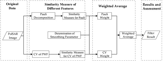
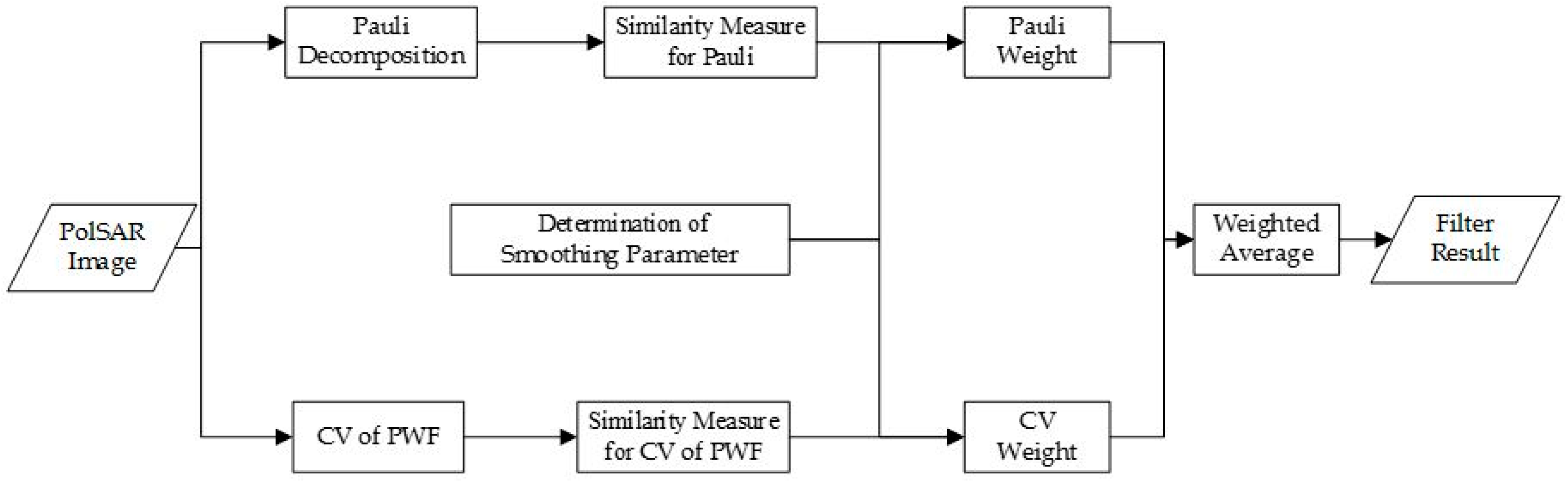
2.3.2. Procedure of Weighted Average

In 2005, Buades et al. [10] proposed a nonlocal mean filter algorithm. The idea of this algorithm is to replace the similarity of individual pixels with the structural similarity in the image, and to estimate the pixel value by using the redundant information. Thus, a large number of nonlocal filtering algorithms have been proposed and achieved good performance of speckle suppression, and the form is expressed as [10]:

$$\widehat{\mathit{u}}\left(x\right)=\frac{1}{Z\left(x,y\right)}{\displaystyle \sum _{y\in \Omega }}w\left(x,y\right)\mathit{u}\left(y\right)$$

(14)

where $\widehat{\mathit{u}}\left(x\right)$ and $\mathit{u}\left(y\right)$ denote the pixel values in noise free and noisy image, respectively. $\Omega$ is the search window. The weight $w\left(x,y\right)$ is computed using the noisy patches, which can be defined as: $w\left(x,y\right)=exp\left(-D\left(x,y\right)/h\right);$ h is the smoothing parameter. $Z\left(x,y\right)$ is the normalization constant, $Z\left(x,y\right)={\displaystyle \sum _{y\in \Omega }}w\left(x,y\right),D\left(x,y\right)$ is the similarity measure between pixel $x$ and $y$.

The speckle-reduced pixel of the PWF is obtained by the linear combination of intensities of ${\left|\mathrm{HH}\right|}^2,{\left|\mathrm{HV}\right|}^2,{\left|\mathrm{VV}\right|}^2$ and a correlation term. Therefore, the $\mathrm{CV}$ based on the PWF is consistent with the statistical properties of a single-channel PolSAR image. Based on the above derivation, the similarity of two patches based on the $C{V}_F$ and the PB can be given as follows: $D_{C{V}_F}\left(x,y\right)={\sum }_{i=1}^M\left(lnC{V}_{F{X}_i}+lnC{V}_{F{Y}_i}-2\ln \left(C{V}_{F{X}_i}+C{V}_{F{Y}_i}\right)\right)$ and $D_{PB}\left(x,y\right)={\sum }_{i=1}^M\ln Q_i={\sum }_{i=1}^M\left(\ln P{B}_{X_i}+\ln P{B}_{Y_i}-2\ln \left(P{B}_{X_i}+P{B}_{Y_i}\right)\right)$.

Correspondingly, according to the NLM filter, the weights for the $C{V}_F$ and the PB are defined as $w_{C{V}_F}\left(x,y\right)=exp\left(\frac{D_{C{V}_F}}{h_{C{V}_F}}\right),w_{PB}\left(x,y\right)=exp\left(\frac{D_{PB}}{h_{PB}}\right)$, the parameter $h$ affects the weight decay. Homogeneous samples should be close in both the $C{V}_F$ and the PB domains. Accordingly, the filter weight is the product of two feature weights and expressed as:

$$w\left(x,y\right)=w_{C{V}_F}\left(x,y\right)·w_{PB}\left(x,y\right)$$

(15)

It should be noted that the three values would be calculated according to the three components of the Pauli basis, and the test of the polarization feature is obtained by summing the three values. Moreover, the polarimetric covariance or coherence matrices are Hermitian positive definite matrices based on the test statistic in [32]. Hence, when the rank of the matrices is less than three, the undefined channel values are discarded and the similarity measure is determined by other channel values.

2.3.3. Determination of Smoothing Parameters

The parameter $h$ controls the degreeof smoothness in the proposed filter. In addition, the speckle reduction is much better with the parameters increasing. In the two similarity measures, we need to set the smoothing parameters of heterogeneity $h_{C{V}_F}$ and polarimetric scattering $h_{PB}$. Ideally, the texture information is desirable to be preserved in the higher heterogeneity region, and smaller smoothing parameters are required. In addition, the larger smoothing parameters are capable of suppressing the speckle in the homogeneous region.

In contrast, heterogeneity describes the complexity of the image. Therefore, the smoothing parameter of heterogeneity $h_{C{V}_F}$ can be determined adaptively according to the reciprocal of the heterogeneity: $h_{C{V}_F}=1/C{V}_F$. To improve the parameter robustness, the mean value of the center patch $C{V}_F$ is used to determine the heterogeneity parameter. Moreover, the parameters relate to the patch size $M$ and the number of looks $L$. The differences between patches increase when the patch size grows, but the effect of speckle is reduced with increasing the number of looks. Thus, the heterogeneity parameter can be defined as:

$$h_{C{V}_F}=log10\left(M\right)/\left(\sqrt{L}C{V}_F\right)$$

(16)

The Pauli parameter is tuned experimentally and given as follows:

$$h_{PB}=Mlog10\left(M\right)/\left(\sqrt{L}\right)$$

(17)

The basic procedure of the proposed method is presented in Algorithm 1 as follows.

Algorithm 1: Nonlocal bilateral filtering based on heterogeneity and scattering.

INPUT: PolSAR image coherence matrix (or covariance matrix).

(1) For each pixel, the weight is calculated according to the test statistic between two patches.

(a) The $\mathit{C}{\mathit{V}}_{\mathit{F}}$ is calculated from the PWF filtered image, and a heterogeneity map is generated.

(b) Calculate the parameter ${\mathit{h}}_{\mathit{C}{\mathit{V}}_{\mathit{F}}}$ and ${\mathit{h}}_{\mathit{P}\mathit{B}}$ according to the $\mathit{C}{\mathit{V}}_{\mathit{F}}$, the number of looks $\mathit{L}$ and the patch size $\mathit{M}$.

(c) The test statistic is measured between two patches of the scalar values including the $\mathit{C}{\mathit{V}}_{\mathit{F}}$ and the Pauli basis of the original image, respectively.

(d) The weights are performed based on the test statistic.

(2) The filtered coherence matrix (or covariance matrix) is performed by the weighted average based on the combination of the weights for the $\mathit{C}{\mathit{V}}_{\mathit{F}}$ and the Pauli basis.

Output: the filtered image.

3. Experiment and Results

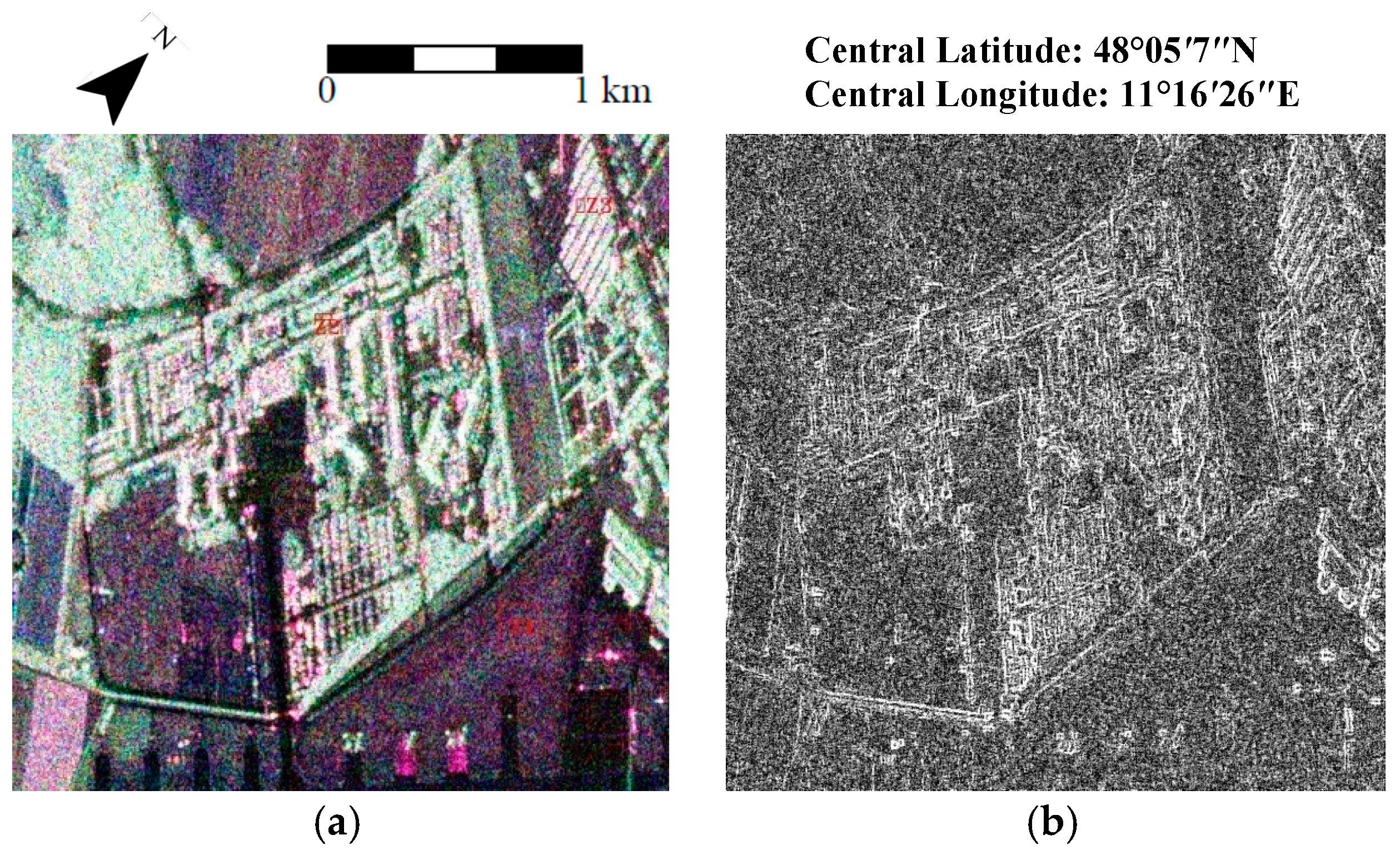
3.1. Description of the Experimental Datasets

The simulated and real PolSAR datasets are utilized in the experiments to evaluate the performance of the proposed filter, including one-look and multilook datasets, respectively. The simulated PolSAR datasets are generated by using Monte Carlo simulation according to the procedure provided by Lee et al. [33]. The given coherent matrices are obtained from the samples of the real PolSAR data, and the regions of different heterogeneity are generated by varying the shape factor in K-distribution [34].

The one-look simulated data with a size of 300 × 300 pixels is mainly composed of field and forest, which is shown in Figure 2a. Additionally, as shown in the red boxes, three isolated points were included to evaluate the preservation of strong targets of the filtered image. The ground truth image is generated by following the method in [35] with the given the coherence matrices and displayed in Figure 2b.The heterogeneity is measured by using the $C{V}_F$. Given the effect of the patch size, the size is set to 3 × 3. Figure 2c shows the corresponding heterogeneity map.

The four-look data includes water body, road, field, forest, and building areas with the dimensions of 300 × 300 pixels, and the Pauli decomposition image is presented in Figure 3a. The corresponding ground truth image and heterogeneity map are shown in Figure 3b,c. As can be seen from the heterogeneity maps in Figure 2c and Figure 3c, the features of the ground targets can be clearly detected, and the boundaries between classes do not spread. The $C{V}_F$ can effectively distinguish between homogeneous and heterogeneous areas and be used to measure the similarity. It should be noted that, except the building area, each ground target is relatively homogeneous with the lower heterogeneity, and the difference between the classes is clearer.

For illustration, two real PolSAR images are employed to validate the performance of the proposed approach: the first real PolSAR dataset is acquired by the AIRSAR system over San Francisco. The region of 400 × 400 pixels is selected from the four-look AIRSAR image, which is mainly composed of water, forest, point targets and urban areas. The Pauli decomposition image of the AIRSAR data is shown in Figure 4a. Correspondingly, the heterogeneity map calculated by $C{V}_F$ is shown in Figure 4b.The second real PolSAR dataset uses a section of the one-look ESAR image over the Oberpfaffenhofen area, where both weak and strong point objects, line, and field areas are included. The Pauli decomposition image and the corresponding heterogeneity map are presented in Figure 5a,b, respectively. It can be seen that the object features such as the building area and the block boundary can be distinguished well.

3.2. Evaluation and Comparision

The filtering experiments are performed and compared by the local and nonlocal filtering methods, respectively. In this paper, the chosen filtering methods include (a) the refined Lee filter; (b) the iterative weight bilateral (ite-bilateral) filter according to the iterative filter weight of the spatial and polarimetric distances; (c) the nonlocal Lee (NL-Lee) filter based on the combination of the test statistics and the preselection; (d) the speckle reducing anisotropic diffusion (SRAD) filter by utilizing the partial differential equations [35,36,37,38]; (e) the MuLog-TV filter of the latest algorithm applying Gaussian denoisers [39]; and (f) the proposed CVPB-NLM filter method.

The size of the sliding window for the refined Lee filter is set to be 7 × 7. The ite-bilateral filter with fiveiterations uses an 11 × 11 window, and the parameters of the weights sensitivity are $h_s=3,h_p=0.6$. The nonlocal Lee (NL-Lee) filter uses a 15 × 15 search window and a 7 × 7 patch with a threshold coefficient of 20. In addition, a 3 × 3 neighborhood patch is set for the sigma filter to preselect more homogeneous region. In addition, the NL-Lee filter requires that the coherency or covariance matrix should be not singular, because the NLM weight employed in the NL-Lee filter is based on Hermitian positive definite matrices [13]. Thus, in this paper, the NL-Lee filter is only applied to multilook PolSAR images. The SRAD filter is implemented with a maximum of 100 iterations and a time step ∆t = 0.1, including an 11 × 11 window for estimating the noise level. For the proposed CVPB-NLM filter method, the same search patch is set to be 15 × 15, with the 3 × 3 heterogeneity and 3 × 3 Pauli patches size, and the parameters are given as Equations (16) and (17).

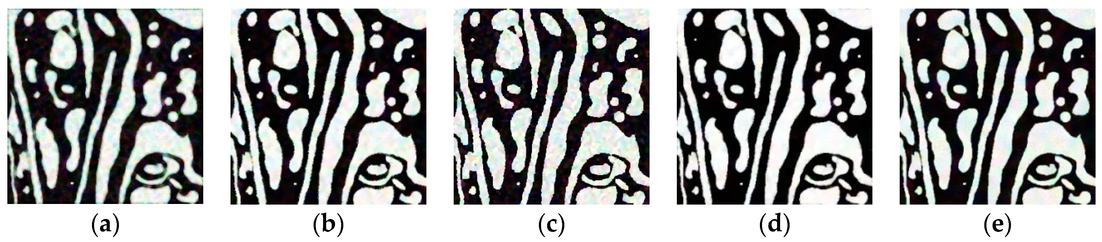
3.2.1. Experiments on Simulated PolSAR Data

In this section, the simulated PolSAR data was employed to quantitatively analyze and evaluate the performance of the proposed approach. As shown in Figure 6 and Figure 7, the different filtering methods can effectively reduce the speckle. Nevertheless, the edges and the texture details were largely smeared by the refined Lee filtering. Meanwhile, a noticeable pixelation effect was introduced. The ite-bilateral filter made a good performance on the speckle reduction, but some discrete points were introduced near the edges. Similarly, the SRAD tended to oversmooth the point targets, which was conducted according to the iterative nature and diffusion tensor. The edges of the proposed filtering and the MuLoG-TV filter seem more continuous with high contrast while speckle was effectively suppressed. As can be seen, the result of the NL-Lee filter was insufficiently smoothed.

Additionally, the performance of the filter results can be quantitatively evaluated according to the reference ground truth image. As mentioned in [35,40], the preservation of the polarimetric and spatial information was analyzed, and the evaluation of the suppression was measured. Specifically, the amplitude and phase of the pixel were denoted by the complex correlation parameters (Ca, Cp). The radiometric parameter was corresponding to the power information (P). The decomposition parameters H/ᾱ/A, including the entropy (H), the anisotropy (A), and the mean alpha angle (ᾱ) were also estimated. These parameters were considered to evaluate the polarimetric information. Then, the absolute relative bias per scattering class was calculated for the filtered images and the ground truth image, and the median of different biases was used to evaluate the preservation of image information. Thus, the smaller value denoted the better ability to retain the information.

The edge preservation degree denoting the spatial information was evaluated according to the ratio of average (EPD-ROA) in the horizontal and vertical directions, respectively [41]. The value close to one indicated good edge preservation. The equivalent number of looks (ENL) was applied to measure the degree of suppression, which was defined as the square ratio of the mean to the standard deviation values in a homogeneous region [40,41,42]. The larger the ENL was, the better the quality of the speckle reduction was. In this experiment, the homogeneous areas of the simulated data were selected from the field and road.

The quantitative evaluation of the filter results was shown in

Table 1. Quantitative evaluation of the simulated PolSAR data.

Data	The One-Look Simulated PolSAR Data
Methods/Indicators	ᾱ	A	H	Ca	Cp	P	ENL	EPI-HD	EPI-VD
Refined Lee	0.007	0.060	0.102	0.585	0.591	0.218	45.942	0.620	0.369
ite-bilateral	0.005	0.138	0.015	0.077	0.544	0.222	53.421	0.710	0.555
SRAD	0.007	0.175	0.052	0.242	0.423	0.489	28.267	0.781	0.862
MuLoG-TV	0.023	0.391	0.070	0.515	0.430	0.164	54.775	0.709	0.602
CVPB-NLM	0.004	0.360	0.031	0.323	0.262	0.129	62.291	0.902	0.575
Data	The Four-Look Simulated PolSAR Data
Methods/Indicators	ᾱ	A	H	Ca	Cp	P	ENL	EPI-HD	EPI-VD
Refined Lee	0.011	0.022	0.016	0.342	0.342	0.063	18.192	0.804	0.715
ite-bilateral	0.004	0.036	0.003	0.031	0.026	0.020	1.134	0.840	0.854
NL-Lee	0.004	0.032	0.003	0.079	0.028	0.017	18.772	0.747	0.913
SRAD	0.012	0.031	0.023	0.484	0.484	0.034	42.951	0.755	0.767
MuLoG-TV	0.016	0.074	0.022	0.444	0.052	0.053	35.108	0.675	0.708
CVPB-NLM	0.002	0.021	0.006	0.055	0.106	0.010	28.517	0.913	0.928

, and the best values are marked in bold. For the one-look simulated data, it can be seen that the proposed CVPB-NLM obtained the best filtering result. The SRAD filter can better preserve the edges and the polarimetric information, while the speckle noise was insufficiently smoothed for the one-look simulated image. Meanwhile, the larger ENL and EPD-ROA indicated that the MuLoG-TV filter and the ite-bilateral filter were able to better suppress the speckle and preserve the edges for the one-look simulated image. For the four-look simulated data, because of the effect of discrete points near the edge, the ite-bilateral filter had the smallest ENL. The comprehensive evaluation of the one-look and four-look simulated data certifies that the proposed CVPB-NLM filter made a better tradeoff between speckle removal and information preservation.

3.2.2. Experiments on Real PolSAR Data

The different filtering results of the AIRSAR image were presented in Figure 8, respectively. As shown in Figure 8b, the ite-bilateral filtering smeared the point targets (as shown the red boxes), and the edges and some tiny details were smoothed. The refined Lee filter preserved the strong points well; however, the weak ones were blurred. In comparison, the NL-Lee filtering obtained slightly improved visual quality and the edges were preserved better, but the speckle noise in the water was significantly higher than the ite-bilateral filtering and the proposed CVPB-NLM filtering. Visually, the performance of the MuLoG-TV filter was better than the NL-Lee filter, and the SRAD filter obtained a good preservation of spatial details. As can be seen, the CVPB-NLM filtering showed the better preservation of the edges and texture information in the forest and building areas, and the speckle noise was effectively suppressed.

For the ESAR image, the corresponding filtered images were shown in Figure 9. We can see that the strong isolated points could be preserved well. Meanwhile, the refined Lee filter blurred the textures and introduced a pixelation effect in the homogeneous regions. The SRAD filtering gave a better detail preservation and the clearer edges. While some details of the ite-bilateral filtered image were removed. As shown, the proposed filter and the MuLoG-TV filter showed better performance of reducing speckle noise while preserving edges.

In the different filtering images, the uniform homogeneous and heterogeneous regions were chosen for computing the ENL and EPD-ROA, which were marked by red rectangles in Figure 4a and Figure 5a. Specifically, the marked Z1 region was located within the homogeneous area and applied to calculate the ENL, the other heterogeneous areas Z2 and Z3 were calculated for the EPD-ROA. In order to analyze and compare the effects on the polarimetric information of different filtering methods, three 40 × 40 homogeneous areas were selected according to [35]. Then, the entire mean of the 40 × 40-pixel areas was assumed to be the reference data. The quantitative evaluation of different filter methods was conducted, which was similar to the evaluation of the simulated data, while the spatial correlation of the real datasets was much higher than the simulated image. The effect of the speckle on the original image was larger, and the entropy (H) of the decomposition parameters could be compared.

Table 2. Quantitative Evaluation of the real PolSAR data.

Data	Method/Indicators	ᾱ	A	Ca	Cp	P	ENL	EPI-HD	EPI-VD
AIRSAR	Refined Lee	0.178	0.658	0.087	0.063	0.119	0.489	0.749	0.969
	ite-bilateral	0.166	0.803	0.097	0.074	0.090	1.388	0.758	0.902
	NL-Lee	0.171	0.777	0.080	0.071	0.070	0.424	0.723	0.918
	SRAD	0.167	0.657	0.098	0.071	0.098	0.810	0.708	0.926
	MuLoG-TV	0.134	0.647	0.232	0.073	0.256	0.732	0.775	0.927
	CVPB-NLM	0.168	0.806	0.096	0.071	0.086	1.224	0.806	0.998
Data	Method/Indicators	ᾱ	A	Ca	Cp	P	ENL	EPI-HD	EPI-VD
ESAR	Refined Lee	0.056	0.411	0.561	0.686	0.245	18.992	0.413	0.788
	ite-bilateral	0.075	0.421	0.330	0.323	0.158	18.522	0.524	0.824
	SRAD	0.075	0.366	1.030	0.710	0.140	12.061	0.941	0.863
	MuLoG-TV	0.080	0.391	0.302	0.210	0.173	28.905	0.505	0.770
	CVPB-NLM	0.075	0.439	0.340	0.260	0.163	22.990	0.623	0.780

presents the quantitative evaluation with the quantitative indicators of the AIRSAR and ESAR images, moreover, the best results are marked in bold. As shown, ENL of different filters was lower for the AIRSAR image, because the selected relatively homogeneous region in water body was nonstationary in the experimental area. For the AIRSAR image, the proposed CVPB-NLM filter obtained the highest EPD-ROA results. In addition, it can be observed that the ite-bilateral filter and the proposed filter had a much larger ENL and indicated strong speckle reduction ability; however, the EPD-ROA of the ite-bilateral filter was significantly lower than the proposed filter. The ENL of the NL-Lee filter showed that it was not smooth enough. Meanwhile, the MuLoG-TV filter showed the best preservation of polarimetric information and a better speckle reduction ability. The quantitative indicators of the SRAD filter showed a good balance between noise removal and information preservation.

The results of the ESAR image exhibited that the CVPB-NLM filter and the MuLoG-TV filter had the better speckle reduction ability. The SRAD filter showed the best preservation of polarimetric information and details information, while the ENL was the lowest. The MuLoG-TV filter showed the best preservation of polarimetric information and speckle reduction ability. Meanwhile, most of the quantitative indicators of the proposed method were better than the other filters. For the real PolSAR data, this proposed filter method and the MuLoG-TV filter achieved a better balance between the speckle suppression and the preservation of the polarimetric information.

Figure 10 and Figure 11 presented the entropy images of the different filtering methods on AIRSAR and ESAR data, which were obtained from H/A/ᾱ polarimetric decomposition [28]. The entropy can describe the polarimetric scattering degree of randomness. As it is shown, the entropy values of the forest areas were high, because of the random scattering process. The homogeneous regions had low degree of scattering randomness. In the building areas, different scattering mechanisms were mixed with the higher entropy values. The refined Lee filter and the SRAD filter preserved the textures in the forest zones, but the built-up regions of the refined Lee filter were blurred for the AIRSAR image. Meanwhile, the NL-Lee filter, the ite-bilateral filter and the MuLoG-TV filter blurred the textures in the forest zones for the AIRSAR image. The proposed method was the one that better preserved the low entropy small spots and lines within both the forest and urban area. The proposed method and the MuLoG-TV filter can distinguish the edges and line targets for the ESAR image, and the homogeneous and heterogeneous regions were clearly observed.

The Canny detector [42] was applied to the HH band of the AIRSAR data, and the results were presented in Figure 12. As shown, the Gaussian filter was used with the standard deviation of 0.5 in the Canny detector for each filtered image. It can be seen that a few edges and details were lost, even the Canny detector was applied to test the multi-look images. Specifically, the proposed CVPB-NLMfilter and the MuLoG-TV filter preserved the coastline better (red box 1). The refined Lee filter and the NL-Lee filter lose the significant information of forest area, while the detected edges of the SRAD filter were clearer (red box 3). The ite-bilateral filter failed to detect the fine details in the left part (red box 2), although a few linear features were visible in the middle of forest areas. In the building region, the detected edges of the NL-Lee filter and the proposed filter were closer, while the small details were preserved better by the proposed filter. Relatively, the MuLoG-TV filter detected the most details, but there are more false edges.

4. Discussion

4.1. Main Features of the Proposed Method

In this paper, the features of the heterogeneity and polarimetric scattering are introduced to the proposed filtering method for PolSAR images. The combination of the extracted features effectively improves the estimation accuracy of the similarity weights. In addition, the influence of the distribution model and the probability density parameter are reduced. The filter makes a good balance between speckle removal and detail preservation.

The first feature of this paper is that the pixel similarity is measured based on scene heterogeneity. The heterogeneity is able to quantitatively and objectively measure the complexity of scenes. Moreover, the heterogeneity is an important parameter reflecting image texture characteristics, which has been widely used in SAR(PolSAR) image segmentation, classification, feature extraction, and filtering processing [29,43,44]. The $\mathrm{CV}$ is the most commonly used heterogeneity test method. In this paper, the $\mathrm{CV}$ is calculated according to the PWF. The accuracy of the heterogeneity can be effectively improved by the $\mathrm{CV}$ based on the PWF ($C{V}_F$). Thus, the $C{V}_F$ is used as the feature to measure the heterogeneity similarity.The Pauli basis is used as the second feature to test the scattering mechanism. In PolSAR images, the components of the Pauli basis can represent the signatures of the objects and have physical meanings to interpret the scattering mechanisms. The Pauli RGB image is commonly applied to display the PolSAR images. Based on the above analysis, the application of the features in the novel filter reduces the dependence on the distribution model and the probability density.

The relevant filtering methods [7,8,9,11,12,13,14] perform the weighted average by measuring the similarity of the statistical target information or spatial distance. The spatial distance is unsuitable for multiplicative speckle noise of the PolSAR image. In addition, the filter results may be affected with a less repeated structure. In this paper, the similarity of the features is deduced according to the test statistic. The proposed filter is performed by using the weighted average of similar pixels.Compared with other filtering methods, this approach integrates the heterogeneity and polarimetric properties to evaluate the pixels similarity and enhance speckle reduction capabilities. Due to the use of target features, the stability of the proposed algorithm is improved, and it is fit for single-look and multi-look PolSAR images.

4.2. Sensitivity Analysis of the Parameters

4.2.1. Sensitivity Analysis of the Smoothing Parameters

In the proposed method, the two smoothing parameters are defined, including heterogeneity $h_{C{V}_F}$ and the Pauli parameter $h_{PB}$. According to the reciprocal of the heterogeneity, the parameter $h_{C{V}_F}$ can be determined adaptively; meanwhile, the patch size $M$ and the number of looks $L$ are included. Thus, for a PolSAR image, the map of the parameter $h_{C{V}_F}$ is determined when the patch size is fixed. Similarly, the Pauli parameter $h_{PB}$ is a function of the patch size $M$ and the number of looks $L$. The Pauli smoothing parameter can be experimentally tuned based on the heterogeneity smoothing parameter. In order to compare with the ground truth, the experimental results based on the simulated PolSAR images are analyzed according to the different Pauli parameter.

Figure 13a presents the maps of the parameter $h_{C{V}_F}$, and the experimental results of the different Pauli smoothing parameters are shown in Figure 13b–d. As can be seen, the values of the edges, point targets and the building areas are significantly smaller than the homogeneous regions, and the parameter $h_{C{V}_F}$ is able to adaptively control the degree of smoothness according to the map. The filtered results based on the Pauli parameters are affected by applying the different Pauli parameters, and in this paper the determined parameter could achieve better performance.

4.2.2. Size of the Patch

The influence of the patch sizes is analyzed for the final results, and the experiments are conducted based on the different patch sizes ranging from 3 × 3 to 11 × 11. For comparison, the experimental results of different patch sizes are shown in Figure 14, Figure 15 and Figure 16. As can be seen, the result shows reasonably good characteristics of preserving edges and scattering properties, andsmall features are much clearer with a larger patch. While, when the smoothing parameters are determined, speckle filtering power is reduced with the increase of the patch. Since, in a larger patch, the difference is greater than in a smaller patch, the pixel targets are regarded as the heterogeneity patches.

The quantitative results of different patch sizes are shown in

Table 3. Filter results of different patch sizes for simulated PolSAR images.

Data/Indicators		ᾱ	A	H	Ca	Cp	P	ENL	EPD-HD	EPD-VD
one-look	3 × 3	0.004	0.360	0.031	0.323	0.262	0.129	62.291	0.691	0.979
	5 × 5	0.004	0.303	0.045	0.292	0.589	0.478	81.982	0.707	0.873
	7 × 7	0.003	0.238	0.078	0.480	0.518	0.751	72.076	0.750	0.860
	9 × 9	0.003	0.317	0.137	0.598	0.608	0.597	61.361	0.821	0.837
	11 × 11	0.003	0.343	0.222	0.603	0.737	0.537	39.299	0.842	0.935
four-look	3 × 3	0.002	0.021	0.006	0.055	0.106	0.010	28.517	0.835	0.913
	5 × 5	0.003	0.013	0.006	0.186	0.216	0.013	16.780	0.775	0.900
	7 × 7	0.004	0.028	0.014	0.308	0.366	0.013	12.542	0.912	0.943
	9 × 9	0.006	0.087	0.033	0.587	0.551	0.008	12.681	0.891	0.978
	11×11	0.009	0.168	0.062	0.957	0.703	0.009	16.365	0.967	0.994

and

Table 4. Filter results of different patch sizes for real PolSAR images.

Data	Indicators	ᾱ	A	Ca	Cp	P	ENL	EPI-HD	EPI-VD
AIRSAR	3 × 3	0.168	0.806	0.096	0.071	0.086	1.224	0.806	0.998
	5 × 5	0.166	0.790	0.098	0.076	0.092	0.621	0.807	0.962
	7 × 7	0.165	0.717	0.098	0.081	0.087	0.978	0.768	0.935
	9 × 9	0.167	0.598	0.100	0.079	0.087	0.995	0.822	0.975
	11 × 11	0.171	0.505	0.103	0.079	0.087	0.437	0.839	0.998
Data	Method/Indicators	ᾱ	A	Ca	Cp	P	ENL	EPI-HD	EPI-VD
ESAR	3 × 3	0.075	0.439	0.340	0.260	0.163	22.990	0.623	0.780
	5 × 5	0.075	0.423	0.368	0.250	0.162	24.652	0.580	0.788
	7 × 7	0.077	0.412	0.356	0.356	0.156	21.900	0.565	0.786
	9 × 9	0.077	0.393	0.614	0.567	0.152	16.090	0.615	0.791
	11 × 11	0.077	0.350	1.108	0.724	0.149	12.540	0.679	0.773

, and the best results are marked in bold. As shown in Table 3, the complex correlation parameters of the simulated data are greatly influenced with the different patch sizes. In addition, there is little difference of the polarimetric information and edge preservation for the simulated image. According to Table 3 and Table 4, the ENL of the filtering method decreases by enlarging the size of the patch. The speckle suppression ability is weakened, while the EPD is slightly greater. In conclusion, the choice of the different patch sizes can affect the speckle reduction of the proposed filter, whereas the preservation of spatial resolution remains relatively stable. Smaller patches could achieve better balance between noise removal and detail preservation.

5. Conclusions

In this paper, an improved filtering method based on the features of the coefficient of variance ($\mathrm{CV}$) and the Pauli basis (PB) is proposed with the framework of the nonlocal mean (NLM) approaches for polarimetric synthetic aperture radar (PolSAR) images. The combination of the features aims to improve the performance to discriminate the ground targets and reduces the dependence on the distribution model and the probability density. Furthermore, the stability of the proposed algorithm is improved, and it is fit for single-look and multi-look PolSAR images based on the similarity weights deduced from the test statistics.

Experiments with simulated data, airborne L-band AIRSAR, and ESAR PolSAR data were conducted to verify the performance of the proposed method. The equivalent number of looks (ENL) and most polarimetric indices of the proposed approach achieved the highest value for the one-look simulated image. For the multi-look simulated data, a better preservation of the polarimetric information, the power information, and the details of the edge preservation degree based on the ratio of average (EPD-ROA) were achieved. For the real PolSAR images, the quantitative indices of the proposed approach were not the highest values. However, the proposed approach achieved a better balance between the speckle filtering and the preservation of the polarimetric information, additionally, the obtained entropy images, and the Canny detector results were able to more effectively distinguish the various objects than other methods.

Future work will integrate more features to enhance the estimation accuracy of the similarity measure. In addition, the metric of the distance between the pixels is important for the proposed filtering. Further research is needed to improve the detection of the weak objects and measure the distance more effectively.

References

1. Lee, J.S. Refined filtering of image noise using local statistics. Comput. Graph. Image Process. 1981, 15, 380–389. [Google Scholar] [CrossRef]
2. Lee, J.S.; Grunes, M.R.; De Grandi, G. Polarimetric SAR speckle filtering and its implication for terrain classification. IEEE Trans. Geosci. Remote Sens. 1999, 37, 2363–2373. [Google Scholar]
3. Lee, J.S. Digital image smoothing and the sigma filter. Comput. Vis. Graph. Image Process. 1983, 24, 255–269. [Google Scholar] [CrossRef]
4. Lee, J.S.; Wen, J.H.; Ainsworth, T.L.; Chen, K.S.; Chen, A.J. Improved sigma filter for speckle filtering of SAR imagery. IEEE Trans. Geosci. Remote Sens. 2009, 47, 202–213. [Google Scholar]
5. Lee, J.-S.; Ainsworth, T.L.; Wang, Y.T.; Chen, K.-S. Polarimetric SAR speckle filtering and the extended sigma filter. IEEE Trans. Geosci. Remote Sens. 2015, 53, 1150–1160. [Google Scholar] [CrossRef]
6. Vasile, G.; Trouve, E.; Lee, J.S.; Buzuloiu, V. Intensity-driven adaptive-neighborhood technique for polarimetric and interferometric parameter estimation. IEEE Trans. Geosci. Remote Sens. 2006, 44, 1609–1621. [Google Scholar] [CrossRef]
7. Tomasi, C.; Manduchi, R. Bilateral filtering for gray and color images. In Proceedings of the 6th International Conference on Computer Vision, Bombay, India, 7 January 1998; pp. 839–846. [Google Scholar]
8. D’Hondt, O.; Guillaso, S.; Hellwich, O. Iterative bilateral filtering of polarimetric SAR data. IEEE J. Sel. Top. Appl. Earth Obs. Remote Sens. 2013, 6, 1628–1639. [Google Scholar] [CrossRef]
9. Alonso-Gonzalez, A.; Lopez-Martinez, C.; Salembier, P.; Deng, X.P. Bilateral distance based filtering for polarimetric SAR data. Remote Sens. 2013, 5, 5620–5641. [Google Scholar] [CrossRef] [Green Version]
10. Buads, A.; Coll, B.; Morel, J.-M. A non-local algorithm for image denoisesing. In Proceedings of the IEEE Computer Society Conference Computer Vision and Pattern Recognition CVPR 2005, San Diego, CA, USA, 20–25 June 2005; Volume 2, pp. 60–65. [Google Scholar]
11. Chen, J.; Chen, Y.; An, W.; Cui, Y.; Yang, J. Nonlocal filtering for polarimetric SAR data: A pretest approach. IEEE Trans. Geosci. Remote Sens. 2011, 49, 1744–1754. [Google Scholar] [CrossRef]
12. Ni, W.P.; Gao, X.B. Despeckling of SAR image using generalized guided filter with Bayesian nonlocal means. IEEE Trans. Geosci. Remote Sens. 2016, 54, 567–579. [Google Scholar] [CrossRef]
13. Zhong, H.; Zhang, J.J.; Liu, G.C. Robust polarimetric SARdespeckling based on nonlocal means and distributed lee filter. IEEE Trans. Geosci. Remote Sens. 2014, 52, 4198–4210. [Google Scholar] [CrossRef]
14. Liu, G.C.; Zhong, H. Nonlocal means filter for polarimetric SAR data despeckling based on discriminative similarity measure. IEEE Geosci. Remote Sens. Lett. 2014, 11, 514–518. [Google Scholar] [CrossRef]
15. Wang, Y.T.; Ainsworth, T.L.; Lee, J.S. Application of mixture regression for improved polarimetric SAR speckle filtering. IEEE Trans. Geosci. Remote Sens. 2017, 55, 453–467. [Google Scholar] [CrossRef]
16. Zhang, L.; Sun, L.; Zou, B.; Moon, W. Fully polarimetric SAR image classification via sparse representation and polarimetric features. IEEE Sel. Top. Appl. Earth Obs. Remote Sens. 2014, 8, 3923–3932. [Google Scholar] [CrossRef]
17. Xie, W.; Jiao, L.C.; Zhao, J. PolSAR image classification via D-KSVD and NSCT-domain features extraction. IEEE Geosci. Remote Sens. Lett. 2016, 13, 227–231. [Google Scholar] [CrossRef]
18. Uhlmann, S.; Kiranyaz, S. Integrating color features in polarimetric SAR image classification. IEEE Trans. Geosci. Remote Sens. 2014, 52, 2197–2216. [Google Scholar] [CrossRef]
19. Chen, B.; Wang, S.; Jiao, L.C.; Stolkin, R.; Liu, H.Y. A three-component fisher-based feature weighting method for supervised PolSAR image classification. IEEE Geosci. Remote Sens. Lett. 2015, 12, 731–735. [Google Scholar] [CrossRef]
20. Lopes, A.; Touzi, R.; Nezry, E. Adaptive speckle filters and scene heterogeneity. IEEE Trans. Geosci. Remote Sens. 1990, 6, 992–1000. [Google Scholar] [CrossRef]
21. Frost, V.S.; Stiles, J.A.; Shanmugan, K.S.; Holtzman, J.C. A model for radar images and its application to adaptive digital filtering of multiplicative noise. IEEE Trans. Pattern Anal. Mach. Intell. 1982, 4, 157–165. [Google Scholar] [CrossRef] [PubMed]
22. Lang, F.K.; Yang, J.; Li, D.R. Adaptive-window polarimetric SAR image speckle filtering based on a homogeneity measurement. IEEE Trans. Geosci. Remote Sens. 2015, 53, 5435–5446. [Google Scholar] [CrossRef]
23. Dellepiane, S.G.; Angiati, E. Quality assessment of despeckled SAR images. IEEE J. Sel. Top. Appl. Earth Obs. Remote Sens. 2014, 7, 691–707. [Google Scholar] [CrossRef]
24. Anfinsen, S.N.; Doulgeris, A.P.; Eltoft, T. Estimation of the equivalent number of looks in polarimetric synthetic aperture radar imagery. IEEE Trans. Geosci. Remote Sens. 2009, 47, 3795–3809. [Google Scholar] [CrossRef]
25. Martino, G.D.; Simone, D.A.; Iodice, A.; Riccio, D. Scattering-based nonlocal means SAR despeckling. IEEE Trans. Geosci. Remote Sens. 2016, 54, 3574–3588. [Google Scholar] [CrossRef]
26. Lee, J.S.; Grunes, M.R.; Schuler, D.L.; Pottier, E.; Ferro, L. Scattering-model-based speckle filtering of polarimetric SAR data. IEEE Trans. Geosci. Remote Sens. 2006, 44, 176–187. [Google Scholar]
27. Liu, L.; Jiang, L.M.; Li, H.Z.; Hu, J.X. Improved scattering-model-based speckle filter in polarimetric SAR data with orientation angle compensation. In Proceedings of the 2011 International Conference on Remote Sensing, Environment and Transportation Engineering, Nanjing, China, 24–26 June 2011; pp. 5026–5029. [Google Scholar]
28. Lee, J.S.; Eric, P. Polarimetric Radar Imaging: From Basics to Application; CRC Press: Boca Raton, FL, USA, 2009; pp. 160–161. [Google Scholar]
29. Xu, Q.; Chen, Q.H.; Yang, S.; Liu, X.G. Superpixel-based classification using k distribution and spatia context for polarimetric SAR images. Remote Sens. 2016, 8, 619. [Google Scholar]
30. Novak, L.M.; Burl, M.C. Optimal speckle reduction in polarimetric SAR imagery. IEEE Trans. Aerosp. Electron. Syst. 1990, 26, 293–305. [Google Scholar] [CrossRef]
31. Lopes, A.; Sery, F. Optimal speckle reduction for the product model inmultilook polarimetric SAR imagery and the Wishartdistribution. IEEE Trans. Geosci. Remote Sens. 1997, 35, 632–647. [Google Scholar] [CrossRef]
32. Conradsen, K.; Nielsen, A.A.; Schou, J. Atest statistic in the complex Wishart distribution and its application to change detection in polarimetric SAR data. IEEE Trans. Geosci. Remote Sens. 2003, 41, 4–19. [Google Scholar] [CrossRef]
33. Lee, J.-S.; Grunes, M.R.; Kwok, R. Classification of multi-look polarimetric SAR imagery based on complex Wishart distribution. Int. J. Remote Sens. 1994, 15, 2299–2311. [Google Scholar] [CrossRef]
34. Khan, S.; Guida, R. On fractional moments of multilook polarimetric whitening filter for polarimetric SAR data. IEEE Trans. Geosci. Remote Sens. 2014, 52, 3502–3512. [Google Scholar] [CrossRef]
35. Foucher, S.; Lopez-Martinez, C. Analysis, evaluation, and comparison of polarimetric SAR speckle filtering techniques. IEEE Trans. Image Process. 2014, 23, 1751–1764. [Google Scholar] [CrossRef] [PubMed]
36. Yu, Y.J.; Acton, S.T. Speckle reducing anisotropic diffusion. IEEE Trans. Image Process. 2002, 11, 1260. [Google Scholar] [PubMed]
37. Foucher, S.; Farage, G.; Benie, G. Polarimetric SAR image filtering with trace-based partial differential equations. Can. J. Remote Sens. 2007, 33, 226–236. [Google Scholar] [CrossRef]
38. Foucher, S.; Farage, G.; Benie, G. Speckle filtering of POLSAR and POLINSAR images using trace-based partial differential equations. In Proceedings of the 2006 IEEE International Geoscience and Remote Sensing Symposium, Denvor, CO, USA, 31 July–4 August 2006; pp. 2545–2548. [Google Scholar]
39. Deledalle, C.-A.; Denis, L.; Tabti, S.; Tupin, F. MuLoG, or How to apply Gaussian denoisers to multi-channel SAR speckle reduction? IEEE Trans. Image Process. 2017, 26, 4389–4403. [Google Scholar] [CrossRef] [PubMed]
40. Nie, X.L.; Qiao, H.; Zhang, B.; Huang, X.Y. A Nonlocal TV-based variational method for PolSAR data speckle reduction. IEEE Trans. Image Process. 2016, 25, 2620–2634. [Google Scholar] [CrossRef] [PubMed]
41. Feng, H.; Hou, B.; Gong, M. SAR image despeckling based on local homogeneous region segmentation by using pixel-relativity measurement. IEEE Trans. Geosci. Remote Sens. 2011, 49, 2724–2737. [Google Scholar] [CrossRef]
42. Leonardo, T.; Sidnei, J.S.; Corina, D.C.; Alejandro, C.F. Speckle reduction in polarimetric SAR imagery with stochastic distances and nonlocal means. Pattern Recognit. 2014, 47, 141–157. [Google Scholar]
43. Yang, S.; Chen, Q.H.; Yuan, X.H.; Liu, X.G. Adaptive coherency matrix estimation forpolarimetric SAR imagery based onlocal heterogeneity coefficients. IEEE Trans. Geosci. Remote Sens. 2016, 54, 6732–6745. [Google Scholar] [CrossRef]
44. Wu, J.; Liu, F.; Jiao, L.C.; Zhang, X.G. Local maximal homogeneous region search for SAR speckle reduction with sketch-based geometrical kernel function. IEEE Trans. Geosci. Remote Sens. 2014, 52, 5751–5764. [Google Scholar]
Figure 1. Overview of the proposed algorithm for PolSAR data.
Remotesensing 09 01043 g001
Figure 2. One-look simulated image used in the experiment: (a) one-look simulated image; (b) one-look ground truth; and (c) one-look heterogeneity map.
Remotesensing 09 01043 g002
Figure 3. Four-look simulated image used in the experiment: (a) four-look simulated image; (b) four-look ground truth; and(c) four-look heterogeneity map.
Remotesensing 09 01043 g003
Figure 4. L-band, multi-look PolSAR image of AIRSAR as the first real dataset used in the experiment: (a) originaldata of AIRSAR; and (b) the heterogeneity image of (a).
Remotesensing 09 01043 g004
Figure 5. Single-look PolSAR image of ESAR as the second real dataset used in the experiment: (a) original data of ESAR; and (b) the heterogeneity image of (a).
Remotesensing 09 01043 g005
Figure 6. Speckle reduction images of the one-look simulated data using different filtering algorithms. (a) refined Lee filter; (b) ite-bilateral filter; (c) SRAD filter; (d) MuLoG-TV filter; and (e) CVPB-NLM filter.
Remotesensing 09 01043 g006
Figure 7. Speckle reduction images of the four-look simulated data using different filtering algorithms: (a) refined Lee filter; (b) ite-bilateral filter; (c) NL-Lee filter; (d) SRAD filter; (e) MuLoG-TV filter; and (f) CVPB-NLM filter.
Remotesensing 09 01043 g007
Figure 8. Speckle reduction images of AIRSAR using different filtering algorithms. (a) refined Lee filter; (b) ite-bilateral filter; (c) NL-Lee filter; (d) SRAD filter; (e) MuLoG-TV filter; and (f) CVPB-NLM filter.
Remotesensing 09 01043 g008
Figure 9. Speckle reduction images of ESAR using different filtering algorithms. (a) refined Lee filter; (b) ite-bilateral filter; (c) SRAD filter; (d) MuLoG-TV filter; and (e) CVPB-NLM filter.
Remotesensing 09 01043 g009
Figure 10. Comparison results of entropy images of AIRSAR. (a) refined Lee filter; (b) ite-bilateral filter; (c) NL-Lee filter; (d) SRAD filter; (e) MuLoG-TV filter; and (f) CVPB-NLM filter.
Remotesensing 09 01043 g010
Figure 11. Comparison results of entropy images of ESAR: (a) refined Lee filter; (b) ite-bilateral filter; (c) SRAD filter; (d) MuLoG-TV filter; and (e) CVPB-NLM filter.
Remotesensing 09 01043 g011
Figure 12. Edges detected by the Canny filter applied to the HH polarization channel of ESAR: (a) refined Lee filter; (b) ite-bilateral filter; (c) NL-Lee filter; (d) SRAD filter; (e) MuLoG-TV filter; and (f) CVPB-NLM filter.
Remotesensing 09 01043 g012
Figure 13. The map of the parameter h C V F and the filtered results of simulated PolSAR images for different Pauli parameter based on a 3 × 3 patch size. (a) The map of the parameter h C V F ; (b) Pauli parameter 0.5   h P B ; (c) Pauli parameter h P B size; and (d) Pauli parameter 2   h P B .
Remotesensing 09 01043 g013
Figure 14. The filtered results of simulated PolSAR images for different patch sizes. (a) 3 × 3 of the patch size; (b) 5 × 5 of the patch size;(c) 7 × 7 of the patch size; (d) 9 × 9 of the patch size; and (e) 11 × 11 of the patch size.
Remotesensing 09 01043 g014
Figure 15. The filtered results of AIRSAR image for different patch sizes. (a) 3 × 3 of the patch size; (b) 5 × 5 of the patch size; (c) 7 × 7 of the patch size; (d) 9 × 9 of the patch size; and (e) 11 × 11 of the patch size.
Remotesensing 09 01043 g015
Figure 16. The filtered results of ESAR image for different patch sizes. (a) 3 × 3 of the patch size; (b) 5 × 5 of the patch size; (c) 7 × 7 of the patch size;(d) 9 × 9 of the patch size; and (e) 11 × 11 of the patch size.
Remotesensing 09 01043 g016