Impact and Suggestion of Column-to-Surface Vertical Correction Scheme on the Relationship between Satellite AOD and Ground-Level PM_2.5 in China

Abstract

As China is suffering from severe fine particle pollution from dense industrialization and urbanization, satellite-derived aerosol optical depth (AOD) has been widely used for estimating particulate matter with an aerodynamic diameter less than 2.5 μm (PM_2.5). However, the correlation between satellite AOD and ground-level PM_2.5 could be influenced by aerosol vertical distribution, as satellite AOD represents the entire column, rather than just ground-level concentration. Here, a new column-to-surface vertical correction scheme is proposed to improve separation of the near-surface and elevated aerosol layers, based on the ratio of the integrated extinction coefficient within 200–500 m above ground level (AGL), using the Cloud-Aerosol Lidar with Orthogonal Polarization (CALIOP)) aerosol profile products. There are distinct differences in climate, meteorology, terrain, and aerosol transmission throughout China, so comparisons between vertical correction via CALIOP ratio and planetary boundary layer height (PBLH) were conducted in different regions from 2014 to 2015, combined with the original Pearson coefficient between satellite AOD and ground-level PM_2.5 for reference. Furthermore, the best vertical correction scheme was suggested for different regions to achieve optimal correlation with PM_2.5, based on the analysis and discussion of regional and seasonal characteristics of aerosol vertical distribution. According to our results and discussions, vertical correction via PBLH is recommended in northwestern China, where the PBLH varies dramatically, stretching or compressing the surface aerosol layer; vertical correction via the CALIOP ratio is recommended in northeastern China, southwestern China, Central China (excluding summer), North China Plain (excluding Beijing), and the spring in the southeast coast, areas that are susceptible to exogenous aerosols and exhibit the elevated aerosol layer; and original AOD without vertical correction is recommended in Beijing and the southeast coast (excluding spring), where the elevated aerosol layer rarely occurs and a large proportion of aerosol is aggregated in near-surface. Moreover, validation experiments in 2016 agreed well with our discussions and conclusions drawn from the experiments of the first two years. Furthermore, suggested vertical correction scheme was applied into linear mixed effect (LME) model, and high cross validation (CV) R² (~85%) and relatively low root mean square errors (RMSE, ~20 μg/m³) were achieved, which demonstrated that the PM_2.5 estimation agreed well with the measurements. When compared to the original situation, CV R² values and RMSE after vertical correction both presented improvement to a certain extent, proving that the suggested vertical correction schemes could further improve the estimation accuracy of PM_2.5 based on sophisticated model in China. Estimating PM_2.5 with better accuracy could contribute to a more precise research of ecology and epidemiology, and provide a reliable reference for environmental policy making by governments.

1. Introduction

Aerosols are important components of the atmosphere, and seriously affect climate change [1], earth radiation forcing [2,3], and air quality [4]. Numerous studies have shown that fine particles (with an aerodynamic diameter of less than 2.5 micrometers) play an important role in visibility reduction [5] and public health [6,7]. With fast industrial development and a rapidly expanding economy over the last 30 years, high concentrations of PM_2.5, which contribute to a large amount of anthropogenic emissions [8] and emergence of secondary aerosols, are the cause of frequent severe haze pollution in China [9]. However, research on the impact of PM_2.5 exposures on health has been hindered by limited PM_2.5 datasets, because the air quality monitoring network had been implemented in China in 2013 [10]. As the national monitoring network can only provide localized PM_2.5 data for a limited region, due to monitoring stations being unavailable or too sparse in most areas, satellite remote sensing provides a potential way to monitor continuous PM_2.5 at a large scale by using aerosol optical depth (AOD) [11]. Expanding ground-measured PM_2.5 to large scale monitoring via satellite-derived AOD in China is, therefore, an urgent necessity.

AOD, which is defined as the integrated light extinction over a vertical path through the atmospheric column, is related to surface loadings of fine particles, to a certain extent [12,13]. Up until now, numerous studies on quantitative relationships between satellite-derived AOD and ground-measured PM_2.5 have been developed all around world, where approaches were developed using statistical analysis models, such as multiple linear regression (MLR), generalized additive model (GAM), neural network model (NNM), geographically weighted regression (GWR) and linear mixed effects (LME), pollutant transport models, such as WRF-Chem, WRF-CMAQ, and nested-grid GEOS-Chem model [14,15,16,17,18,19,20,21,22]. To improve the understanding of the relationship between satellite-derived AOD and ground-measured PM_2.5, geographical (i.e., altitude, population density, traffic density, land usage, etc.) and meteorological factors (i.e., temperature, relatively humidity, wind speed, rainfall, planetary boundary layer height (PBLH), etc.) have been included as auxiliary elements [17,18,23,24]. PBLH has been considered to be a key factor influencing the direct relationship between satellite-derived AOD and ground-level PM_2.5, since AOD is the column integral of the aerosol extinction coefficient in vertical distribution of the total atmosphere, while PM_2.5 is the surface measurement [25]. Some researchers suggested that aerosol integration from the top of the atmosphere (TOA) down to the surface could be simplified by division of PBLH under the assumption that aerosols distribute homogeneously under PBL [12]. The assumption of an evenly mixed aerosol under PBL and abundant aerosol above PBL where extinction decreases exponentially with altitude, was also established, thus the values of AOD normalized by PBLH could be regarded as extinction at surface level [25,26]. However, has the satellite derived PM_2.5 via PBLH correction reached its intended surface? Koelemeijer et al. discovered higher correlations between PM_2.5 and AOD divided by the height of the mixing layer, due to vertical mixing leading to dilution of surface concentrations [12]. Han et al. found that PM_2.5 was overestimated when using the total AOD without removing large aloft-layer-AODs when investigating the influence of aloft aerosol-plumes on the AOD–PM_2.5 relationship [27]. Li et al. used CALIPSO extinction profile data to study the impacts of aerosol vertical distribution, and identified seasonal variations in aerosol vertical distribution due to seasonal changes in mixing height, which likely generated the seasonal relationship between low level CALIPSO AOD and PM_2.5, and the seasonal discrepancies in the correlation between PM_2.5 and column AOD from MODIS, MISR, SeaWiFS and OMI [28]. Nevertheless, such research has not been conducted in large areas in China. Since there exist variable terrain conditions from the Tibetan plateau and northwest deserts to the eastern plains [29], and the complex climate controlled by seasonal monsoon system and multi-directional jet stream in China [30], combined with multiple aerosol sources from anthropogenic emissions and natural dust aerosol, aerosol concentrations vary dramatically in both horizontal and vertical dimensions [31,32]. Methods for conducting vertical correction on the satellite column AOD for better correspondence with ground-level PM_2.5 is an urgent issue to solve.

In this study, we first proposed a new vertical correction scheme for satellite-derived AOD, based on the CALIOP profile data for improved separation of the near-surface aerosol layer, further improving the relationship between satellite-derived AOD and ground-measured PM_2.5. Then, the distributions of the annual average of ground-measured PM_2.5 and satellite-derived AOD from 2014 to 2015 were measured, combined with the analysis of the relationship between ground-measured PM_2.5 and satellite-derived AOD. Moreover, comparisons between the new vertical correction scheme by CALIOP and the classic vertical correction via PBLH were conducted, combined with the original relationship between satellite-derived AOD and ground-measured PM_2.5 for reference. Besides, according to the discussions and analyses on the effectiveness of vertical correction, with comprehensive consideration of the influential factors of terrain, climate, meteorology, and aerosol transmission, we recommended a corresponding vertical correction scheme in different regions of China to improve accuracy of estimating ambient PM_2.5 via satellite AOD. In addition, the validation experiments using above three vertical correction methods respectively in six regions were carried out in 2016 to verify the discussions and conclusions. Finally, in order to evaluate the effectiveness of recommended vertical correction scheme, the comparison between the original situation and the revised situation after vertical correction was conducted based on LME model. Furthermore, the accurate distributions of PM_2.5 with a large geographical coverage could not only effectively estimate air quality, but also make a significant contribution to the research on ecology, health and epidemiology, and provide a reference for the environmental policy making by the government [33].

2. Materials and Methods

2.1. Data and Preprocessing

2.1.1. Ground-Measured PM_2.5

Ground PM_2.5 data provided by the air quality monitoring network in China were measured using the tapered element oscillating microbalance method (TEOM) or the β-attenuation method [34]. Figure 1 shows the geographic distribution of monitoring sites within the scope of each provincial capital. All hourly ground-measured PM_2.5 data from 1 January 2014 to 31 December 2015 were obtained from the China Environmental Monitoring Center (CEMC) website (http://113.108.142.147:20035/emcpublish/) [35].

2.1.2. Satellite-Derived AOD from MODIS

The Moderate resolution Imaging Spectroradiometer (MODIS) onboard Terra and Aqua, which cross the equator at approximately 10:30 a.m. and 1:30 p.m. local time (LT), respectively, were used to monitor atmospheric aerosols. The AOD products, one of the MODIS Collection 6 (C6) datasets released in recent years, are proven to satisfy the requirements for validating accuracy against the ground measurements of sun photometers from the Aerosol Robotic Network (AERONET) [36,37]. The MODIS C6 AOD was retrieved from the Dark Target (DT) and Deep Blue (DB) algorithms, and the DB algorithm which makes up for the defect of DT algorithm, expanded the application to cover urban and desert surfaces with high reflectance. Moreover, the C6 new generation DB algorithm improved the clouding screening, NDVI-dependent MODIS surface reflectance database, dust aerosol model selection and quality flag selection procedures when compared to C5.1 DB algorithm, which significantly improved the quality of AOD retrievals over regions with mixed vegetated and non-vegetated surfaces [38]. The Aqua AOD datasets (MYD04) and Terra AOD datasets (MOD04) in a Hierarchical Data Format (HDF) used in this study are available from NASA’s LAADS website (http://ladsweb.nascom.nasa.gov/) [39].

During the daytime, the Terra passes the equator in the morning while the Aqua passes the equator in the afternoon, so the average of the observations of these two satellites was used as the daily value. To improve spatial coverage, the 3 km DT AOD were merged with the 10 km DB AOD based on the rule that DB AOD are used merely in places where DT AOD are not available. After fusion, MODIS AOD was unified to the spatial resolution of 3 km. To eliminate cloud pollution, only the MODIS AOD values when its cloud fraction equals to zero were used in our analyses. To ensure accuracy, only data that were up to the required quality assurance (QA) were used (QA flag = 3 for both DT and DB) [38,40].

2.1.3. CALIOP Data

The Cloud-Aerosol Lidar with Orthogonal Polarization (CALIOP) is a lidar on the Cloud-Aerosol Lidar and Infrared Pathfinder Satellite Observations (CALIPSO) platform, providing high-resolution vertical profiles of aerosols and clouds. In this study, version 3.30 Level 2 aerosol profile products at daytime (CAL_LID_L2_05kmAPro-Prov-V3-30), which contain column AOD (Column_Optical_Depth_Aerosols_532) and have an extinction coefficient of 0.532 μm (Extinction_Coefficient_532) with a vertical resolution of 60 m under 20 km above mean sea level (MSL), were obtained from the NASA CALIPSO website (https://www-calipso.larc.nasa.gov/) [41,42].

2.1.4. Meteorological Data

The Goddard Earth Observing System Data Assimilation System GEOS-5 Forward Processing (GEOS 5-FP, ftp://rain.ucis.dal.ca) was used for this analysis. GEOS 5-FP has a spatial resolution in China of 0.25° latitude × 0.3125° longitude. This study extracts the hourly PBLH meteorological data between 2 UTC and 6 UTC, corresponding to Aqua and Terra crossing time (10:00 LT–14:00 LT) [43].

2.1.5. Data Preprocessing and Integration

Since the above datasets have different temporal and spatial resolutions, all datasets were reprocessed to achieve spatial-temporal matching before the following analyses and discussions. Since Terra and Aqua cross the equator at 10:30 a.m. and 1:30 p.m. respectively, the daily PM_2.5 data were calculated by averaging hourly PM_2.5 observations measured from 10:00 a.m. to 2:00 p.m. For the merged MODIS AOD (briefly introduced in Section 2.1.2), the nearest AOD pixel over a window size of 3 × 3 centered at a given air quality monitoring site station, was extracted to match the measured PM_2.5 value. The similar collocation method was used for meteorological data to match PM_2.5 data.

We averaged all CALIOP ratios within a 100-km radius of a given PM_2.5 station to represent the matched CALIOP ratio. For example, we applied a 100-km search radius at an air quality monitoring site to extract all CALIOP profiles within the region and calculate their corresponding ratios. After removing the maximum and minimum five percentiles, the remaining ratios were then averaged to obtain the matched CALIOP ratio by the inverse distance weighting (IDW) method. To obtain a representative CALIOP ratio around a PM_2.5 site, it is essential to ensure approximately 0.2 of the total profiles within the 100-km radius circle centered on a PM_2.5 site.

2.2. Methodology

2.2.1. Vertical Correction via PBLH

Since AOD is the column integral of the aerosol extinction coefficient in the total atmosphere vertical distribution, while PM_2.5 is the surface measurement, it is not rigorous to study the relationship between satellite-derived AOD and ground-measured PM_2.5 directly. Under the assumption that aerosols distribute homogeneously below PBLH, a classical vertical correction equation had been used to determine the revised satellite-derived AOD in previous studies [12,25].

$$\mathrm{Revised} \mathrm{AOD}=\frac{\mathrm{AOD}}{\mathrm{PBLH}}$$

(1)

2.2.2. Vertical Correction via Near-Surface Ratio by CALIOP

CALIOP provides accurate information of aerosol vertical distributions, so the extinction coefficient profiles measured by CALIOP were adopted for a more accurate vertical correction of the satellite-derived AOD column. According to Toth’s study on the contiguous United States, we also conducted a sensitivity experiment to determine the optimal height range to represent the near-surface layer through changing the height range of the AOD used between 200–300 m above ground level (AGL) and 200–1000 m (AGL) in 100-m interval in China [44]. In our results, the variation in height had little effect on the relationship between the corrected AOD and ground-measured PM_2.5 throughout China, which is similar to Toth’s results that altering the height range of the AOD used slightly influenced the correlation between the revised AOD and ambient PM_2.5 over the contiguous United States. Considering that the extinction coefficients near the surface were susceptible to ground flash contamination [41], approximately 200–500 m AGL was therefore chosen to represent the near-surface layer, which is consistent with previous studies [44]. The near-surface ratio was defined as:

$$\mathrm{Ratio}=\frac{{\mathrm{AOD}}_{200 - 500}}{{\mathrm{AOD}}_{\mathrm{C},\mathrm{column}}}$$

(2)

where ${\mathrm{AOD}}_{200 - 500}$ represents the integral of the aerosol extinction coefficient obtained through CALIOP vertically from 200 m to 500 m AGL; and ${\mathrm{AOD}}_{\mathrm{C},\mathrm{column}}$ represents the integral of the aerosol extinction coefficient obtained through CALIOP in the total vertical column. Therefore, the vertical correction methods using the CALIOP near-surface ratio are as follows:

$$\mathrm{Revised}\_\mathrm{AOD}=\mathrm{Ratio}\times \mathrm{AOD}$$

(3)

where $\mathrm{AOD}$ represents MODIS AOD, $\mathrm{Revised}\_\mathrm{AOD}$ is the AOD vertical corrected by CALIOP. To ensure the accuracy of the CALIOP ratio, only data that met the following criteria were used in this study: (1) the atmospheric feature type is aerosol other than cloud; (2) the value of extinction coefficient is valid; and (3) the values used for calculation were above ground level (Digital elevation model − Mean sea level ≥ 0).

2.2.3. Correlation via Pearson Coefficient

As a classical linear correlation coefficient, the Pearson correlation coefficient (R) is used to reflect the extent to which two variables have a linear correlation. The coefficient of determination (R²) could not reflect a negative correlation between two variables, and while there was a situation where satellite-derived AOD could not correspond well with local ground particulate matter in some areas, therefore, R was chosen to represent the correlation between satellite-derived AOD and ground-measured PM_2.5. The formula of Pearson correlation coefficient is as follows:

$$\mathrm{R}=\frac{1}{\mathrm{N}}{\displaystyle \sum }_{i = 1}^{\mathrm{N}}(\frac{{\mathrm{X}}_i-\overline{\mathrm{X}}}{{\mathrm{S}}_{\mathrm{X}}})(\frac{{\mathrm{Y}}_i-\overline{\mathrm{Y}}}{{\mathrm{S}}_{\mathrm{Y}}})$$

(4)

where $\mathrm{N}$ represents the sample size; ${\mathrm{X}}_i,{\mathrm{Y}}_i$ represent the variables respectively at location $i$; $\overline{\mathrm{X}}$, $\overline{\mathrm{Y}}$ are the average of the two variables, respectively; and ${\mathrm{S}}_{\mathrm{X}}$, ${\mathrm{S}}_{\mathrm{Y}}$ are the standard deviation of two variables respectively.

2.2.4. Linear Mixed Effect Model (LME) and Cross Validation (CV)

Since LME model was developed to explain day variability of PM_2.5-AOD relationship [45], numerous studies had showed the effectiveness of LME model to improve the correlation between PM_2.5 and AOD [19,24,46]. To verify the reliability of the conclusions, a single-variable linear mixed effect model, with a single independent variable, AOD, had been developed in this study. The model structure is shown as follow:

$$\begin{array}{c}{\mathrm{PM}}_{2.5,st}=\left(a+a_{Day}^{\prime }\right){\mathrm{AOD}}_{st}+b+b_{Day}^{\prime }+ϵ\\ a_{Day}^{\prime }~\mathrm{N}\left(0,D_1\right), b_{Day}^{\prime }~\mathrm{N}\left(0,D_2\right), ϵ~\mathrm{N}\left(0,{\sigma }^2\right)\end{array}$$

(5)

where ${\mathrm{PM}}_{2.5,st}$ is the daily average measured PM_2.5 at air quality monitoring site $\mathrm{s}$ on day $\mathrm{t}$; ${\mathrm{AOD}}_{\mathrm{st}}$ is the corresponding AOD at site $\mathrm{s}$ on day $\mathrm{t}$; $a$ is the fixed slopes for AOD and $a_{Day}^{\prime }$ is the random slopes for each day of AOD; $b$ is the fixed intercept and $b_{Day}^{\prime }$ is the random intercept for each day with available matchups in modeling two years data; and $\mathsf{\epsilon }$ is the error term and has independent normal distribution with equal variance and a mean of zero. The random terms have normal distributions. $D_1$ and $D_2$ are variance-covariance matrix for the day-specific random effects ($a_{Day}^{\prime }$ and $b_{Day}^{\prime }$). The fixed effect coefficients including the fixed slopes ($a$) and the fixed intercept ($b$), show the average effect of AOD on PM_2.5 during the study days, while random effect coefficients including the random slopes ($a_{Day}^{\prime }$) and the random intercept ($b_{Day}^{\prime }$), represent daily variability of PM_2.5-AOD relationship.

A 10-fold CV method has been selected in this study to evaluate LME models performance by comparing the estimated PM_2.5 against the measured PM_2.5 [47]. The two-year dataset was partitioned into 10 folds, and nine folds were used to calibrate the model while the remaining one fold was retained for validation in each CV circle. After 10 cycles of this process, all dataset was validated. In this CV process, the regression equation, decision coefficient R², root mean square error (RMSE, μg/m³) and total count of test points (N) were calculated to validated the performance of the model.

3. Results

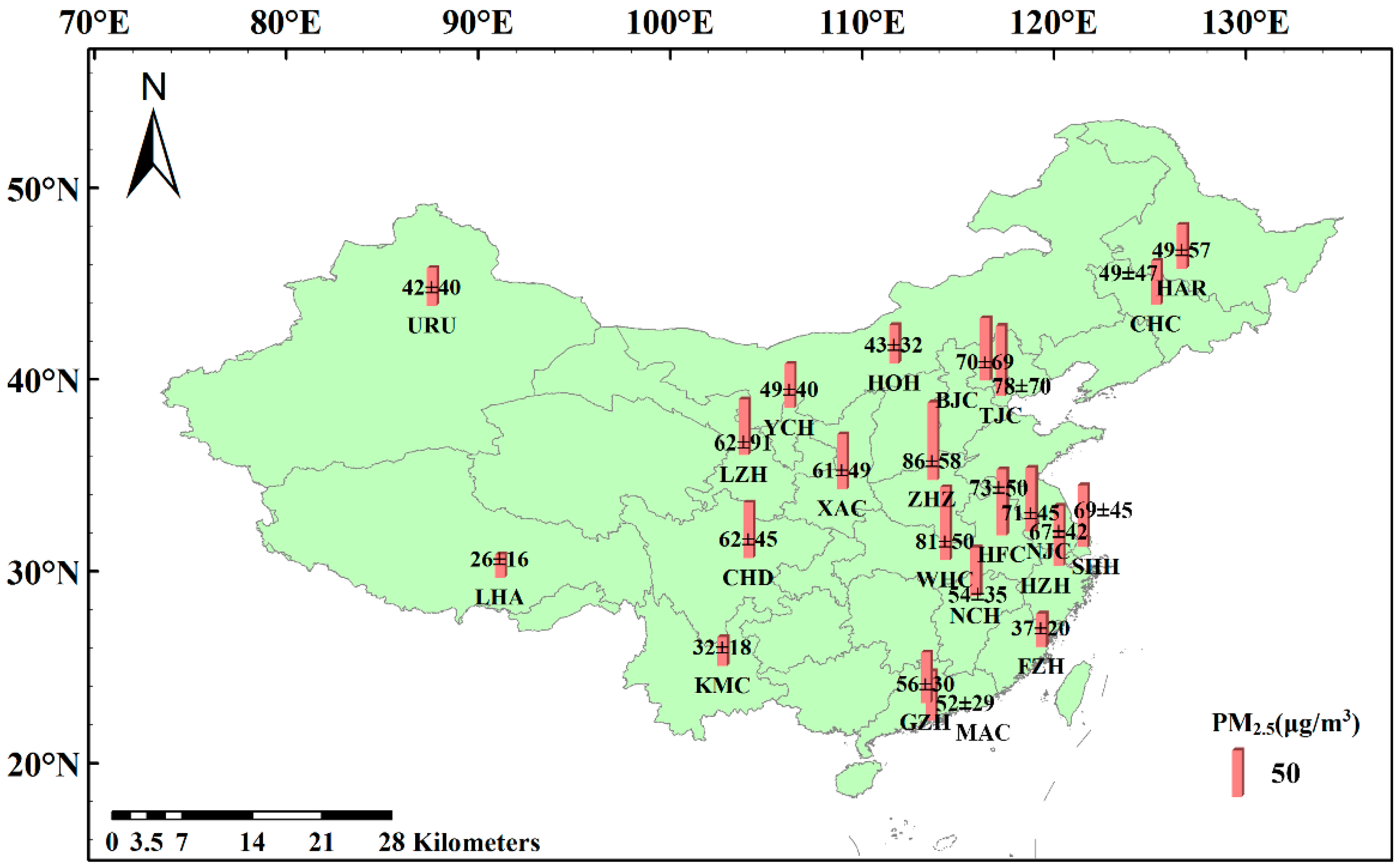
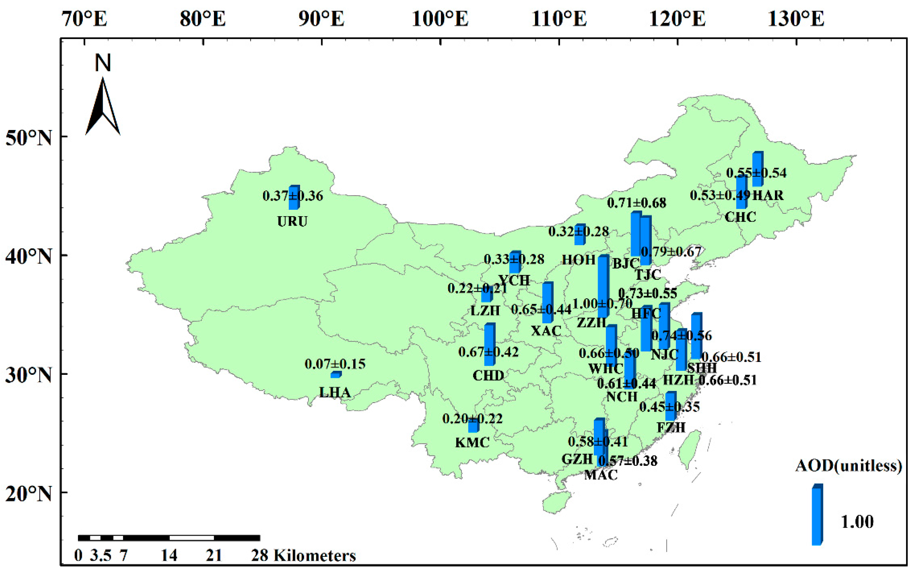
3.1. The Spatial Distributions of PM_2.5 and AOD over China from 2014 to 2015

Figure 2 shows the distribution of the annual PM_2.5 average throughout China from 2014 to 2015. The annual average of PM_2.5 across China varied from 26 μg/m³ to 86 μg/m³, with a maximum daily PM_2.5 average of 3756 μg/m³ in Lanzhou (LZH), and a minimum daily average of 1 μg/m³, observed in several regions on the cleanest days. From an annual perspective, the annual average PM_2.5 of all the provincial capitals were beyond the World Health Organization (WHO) Interim target-2 (IT-2), with 25 μg/m³ PM_2.5 [48], while only Lhasa (LHA) and Kunming (KMC) were lower than the WHO IT-1 standard, with 35 μg/m³ PM_2.5, because of lower anthropogenic aerosol emissions due to lower population density and fewer industrial activities in these regions. From a daily perspective, the percentage of days in two years that satisfied the WHO IT-3 daily standard for PM_2.5 (37.5 μg/m³) ranged from 17 to 81%, while the percentage of days that satisfied the WHO IT-2 daily standard for PM_2.5 (50 μg/m³) ranged from 29 to 92%, and the percentage of days that satisfied the WHO IT-1 daily standard for PM_2.5 (75 μg/m³) ranged from 52 to 98% [48]. It was also identified that the relatively high percentages were mainly observed in northeastern and northwestern China, while the relatively low percentages were observed in Central China and the North China Plain. Through the above analysis, it was demonstrated that most regions of China suffered from severe fine particle pollutions. As illustrated in Figure 3, the spatial distribution of the annual average AOD was consistent with ground-measured PM_2.5, to a certain extent, from 2014 to 2015. The annual averages of AOD ranged from 0.07 to 1.00. Relatively low annual averages of AOD were observed in northwestern and northeastern China, while high annual averages of AOD were observed in the North China Plain and Central China.

3.2. The Relationship between PM_2.5 and AOD throughout China

As shown in

Table 1. The descriptive statistics of PM_2.5 (annual average value ± standard deviation, unit: μg/m³) and AOD (annual average value ± standard deviation, unit: unitless), the linear regression function and the Pearson correlation coefficient (R) of PM_2.5 and AOD, and the data groups (N) involved in the calculation throughout China from 2014 to 2015 are shown, combined with the abbreviations, locations (unit: degree) and terrain height (unit: m) of selected provincial capitals.

Provincial Capital	Longitude	Latitude	Terrain Height (m)	PM2.5	AOD	Y = PM2.5; x = AOD	R	N
LHA	91.11	29.66	4198	26 ± 16	0.07 ± 0.15	Y = −17.7x + 27.5	−0.16	171
URU	87.56	43.84	745	42 ± 40	0.37 ± 0.36	Y = 8.3x + 39.3	0.07	1818
HOH	111.66	40.83	1207	43 ± 32	0.32 ± 0.28	Y = 6.4x + 41.1	0.06	2298
YCH	106.21	38.50	1197	49 ± 40	0.33 ± 0.28	Y = 10.4x + 46.1	0.07	4290
LZH	103.82	36.06	2009	62 ± 91	0.22 ± 0.21	Y = 21.4x + 58.6	0.09	1916
HAR	126.66	45.77	135	49 ± 57	0.55 ± 0.54	Y = 54.5x + 16.9	0.60	2575
CHC	125.31	43.90	208	49 ± 47	0.53 ± 0.49	Y = 39.9x + 28.1	0.41	2169
BJC	116.40	39.93	10	70 ± 69	0.71 ± 0.68	Y = 66.4x + 22.7	0.66	5331
TJC	117.21	39.14	5	78 ± 70	0.79 ± 0.67	Y = 54.6x + 34.8	0.52	4381
HFC	117.28	31.87	40	73 ± 50	0.73 ± 0.55	Y = 36.4x + 46.4	0.40	2752
ZHZ	113.65	34.76	103	86 ± 58	1.00 ± 0.70	Y = 32.9x + 53.5	0.39	5011
WHC	114.32	30.58	18	81 ± 50	0.66 ± 0.50	Y = 50.1x + 47.7	0.50	3074
NJC	118.78	32.06	17	71 ± 45	0.74 ± 0.56	Y = 29.8x + 49.0	0.37	6683
NCH	115.89	28.69	74	54 ± 35	0.61 ± 0.44	Y = 32.6x + 34.6	0.41	2274
XAC	108.95	34.28	638	61 ± 49	0.65 ± 0.44	Y = 31.2x + 40.2	0.28	6534
SHH	121.49	31.25	5	69 ± 45	0.73 ± 0.47	Y = 37.6x + 41.6	0.39	5970
FZH	119.33	26.05	212	37 ± 20	0.45 ± 0.35	Y = 13.9x + 31.0	0.24	1728
GZH	113.31	23.12	21	56 ± 30	0.58 ± 0.41	Y = 33.7x + 36.8	0.45	3939
HZH	120.22	30.26	4	67 ± 42	0.66 ± 0.51	Y = 64.3x + 35.4	0.61	4253
MAC	113.56	22.20	22	55 ± 29	0.57 ± 0.38	Y = 28.6x + 39.0	0.37	3311
CHD	104.07	30.68	530	62 ± 45	0.67 ± 0.42	Y = 48.6x + 29.5	0.45	1796
KMC	102.71	25.05	2089	32 ± 18	0.20 ± 0.22	Y = 24.5x + 27.3	0.30	2002

, a linear regression on ground-measured PM_2.5 and original satellite-derived AOD was performed and the Pearson correlation coefficient (R) was calculated accordingly, combined with the descriptive statistics of PM_2.5 and AOD, as well as the location and terrain height of selected provincial capitals. In this study, over 1700 data groups were collected for calculation and analysis in most of the selected regions, excluding some regions in the north and the plateau due to problems in satellite AOD retrieval on snow-covered surfaces. From the Tibetan plateau and northwestern deserts to the eastern plains, the linear regression function varied greatly throughout the whole country, while the Pearson correlation coefficient (R) ranged from −0.16 to 0.66. Particularly low Pearson correlation coefficients (R) were observed ranging from approximately −0.16 to 0.09 in the northwestern regions, with the regression functions greatly varying in the slopes, from −17.7 to 21.4, and the Pearson correlation coefficient was negative (−0.16) in Lhasa, due to problems in satellite AOD retrieval on a snow-covered surface. Meanwhile, in the southeastern coast, an area susceptible to the influence of monsoons and airflows, the Pearson correlation coefficients (R) varied greatly from 0.24 to 0.61, with slopes ranging from 13.9 to 64.3, and the intercepts ranging from 31.0 to 41.6. In addition, similar Pearson correlation coefficients (R) of approximately 0.40 were observed in Central China, and the analogous values of the slopes and intercepts were approximately 32.9 and 45.9, respectively, which attributes to similarities in aerosol components and analogous weather conditions. In summary, the relationship between the original satellite-derived AOD and ground-measured PM_2.5 varied significantly throughout China, based on multifarious ecosystems [29].

4. Discussion

4.1. The Recommended Vertical Correction Schemes

For the whole of China,

Table 2. The seasonal Pearson correlation coefficient (R) of PM_2.5 and Original satellite-derived AOD, Revised AOD by CALIOP ratio, Revised AOD by PBLH. The optimal values of Pearson correlation coefficient were bolded. Spring includes March, April and May; summer includes June, July and August; autumn includes September, October and November; and winter includes December, January and February.

Region	Provincial Capital	from 2014 to 2015			Spring			Summer			Autumn			Winter
		Original	Ratio	PBLH	Original	Ratio	PBLH	Original	Ratio	PBLH	Original	Ratio	PBLH	Original	Ratio	PBLH
Northwest	LHA	−0.16	-	−0.15	−0.35	-	−0.28	−0.30	-	−0.17	−0.14	-	−0.13	−0.25	-	−0.19
	URU	0.07	0.14	0.37	0.18	0.07	0.48	0.16	0.23	0.23	0.12	0.09	0.32	−0.11	-	0.04
	HOH	0.06	0.27	0.44	0.40	0.40	0.49	0.55	0.25	0.57	0.12	0.12	0.25	0.35	0.36	0.60
	YCH	0.07	0.07	0.40	0.36	0.22	0.41	0.25	0.24	0.27	0.17	0.11	0.39	0.37	0.51	0.51
	LZH	0.09	0.06	0.13	0.18	0.31	0.29	0.41	0.44	0.44	0.20	0.11	0.32	0.01	0.05	0.08
Northeast	HAR	0.60	0.61	0.59	0.39	0.52	0.36	0.76	0.84	0.70	0.65	0.71	0.65	-	-	-
	CHC	0.41	0.86	0.36	0.54	0.55	0.52	0.67	0.93	0.61	0.50	0.72	0.46	0.41	0.49	0.17
North China Plain	BJC	0.66	0.58	0.56	0.69	0.65	0.56	0.72	0.51	0.61	0.80	0.80	0.56	0.72	0.55	0.59
	TJC	0.52	0.72	0.58	0.61	0.77	0.57	0.67	0.70	0.59	0.64	0.88	0.61	0.61	0.68	0.54
Central China	HFC	0.40	0.67	0.57	0.30	0.59	0.48	0.79	0.39	0.73	0.53	0.56	0.54	0.51	0.71	0.57
	ZHZ	0.39	0.55	0.42	0.44	0.51	0.27	0.51	0.50	0.33	0.54	0.65	0.63	0.63	0.63	0.42
	WHC	0.50	0.69	0.60	0.46	0.52	0.46	0.75	0.38	0.67	0.37	0.50	0.38	0.51	0.76	0.55
	NJC	0.37	0.82	0.48	0.29	0.45	0.44	0.70	0.51	0.69	0.30	0.30	0.30	0.53	0.89	0.54
	NCH	0.41	0.69	0.42	0.46	0.47	0.38	0.77	0.76	0.68	0.35	0.72	0.38	0.42	0.63	0.34
	XAC	0.28	0.49	0.48	0.26	0.50	0.41	0.62	0.59	0.37	0.49	0.49	0.49	0.50	0.84	0.52
Southeastern coast	SHH	0.39	0.45	0.34	0.35	0.48	0.28	0.50	0.70	0.38	0.58	0.58	0.27	0.54	0.53	0.41
	FZH	0.24	0.18	0.21	0.39	0.70	0.39	0.35	-	0.24	0.34	-	0.15	0.33	-	0.25
	GZH	0.45	0.27	0.44	0.34	0.62	0.30	0.32	-	0.31	0.38	0.08	0.31	0.60	0.29	0.52
	HZH	0.61	0.58	0.48	0.48	0.69	0.44	0.70	0.20	0.63	0.38	0.16	0.37	0.60	0.52	0.57
	MAC	0.37	0.20	0.29	0.28	0.63	0.19	0.35	-	0.24	0.33	0.20	0.28	0.58	0.20	0.49
Southwest	CHD	0.45	0.89	0.52	0.54	0.56	0.38	0.58	0.71	0.46	0.68	0.70	0.44	0.52	0.92	0.56
	KMC	0.30	0.40	0.32	0.44	0.70	0.40	0.48	-	0.03	0.22	0.98	0.14	0.15	0.35	0.31

shows the seasonal and annual correlations between ambient PM_2.5 and original satellite-derived AOD, ambient PM_2.5 and vertically revised AOD by PBLH, and ambient PM_2.5 and vertically revised AOD by CALIOP ratios. Considering the influential factors of terrain, climate, meteorology, and aerosol transmission, the effectiveness of the vertical correction on satellite-derived AOD has been discussed according to different regions divided by the geographical distributions of monsoons, temperature, humidity and air density, as well as the interrelationships between various types of natural geographic phenomena [49].

In northwestern China, AOD vertically revised by PBLH is more closely related to ground-measured PM_2.5 than the original relationship, and the relationship after vertical correction by the CALIOP ratio. In our collected PBLH datasets of the two years, the PBLH in northwest possessed a large span from 50 to 2800 m and had the largest standard deviation when compared to other regions of china, which is consistent with previous research finding that the boundary layer height varied dramatically due to high frequencies of temperature variation and surface pressure change, combined with the climatologically strong near-surface wind and intense solar radiation in northwestern China [50,51]. Assuming that aerosols are homogeneous under PBL, changes in PBLH could stretch or compress the surface aerosol layer, further influencing the density of aerosols, which led to the discrepancies of PM_2.5 with column AOD [26]. Therefore, after vertical correction via PBLH, the influence of the dramatic changes in boundary layer height could be eliminated to a certain extent, and it is suggested that the AOD vertically revised via PBLH should be used for the estimation of ground-level PM_2.5 in the northwest.

In the North China Plain, the relationship between ambient PM_2.5 and AOD vertically revised by CALIOP ratio was optimal in Tianjin (TJC). Based on two-year CALIOP aerosol profiles data, the existence of valid extinction coefficient values in higher atmospheric layer indicated that the elevated aerosol layer was inclined to appear in this region. Considering aerosol transmission in the North China Plain, Tianjin was significantly affected by air masses that originated from Mongolia and the North China Plain regions, which led to the emergence of elevated aerosol levels, further forming the combined influence of exogenous aerosols and local aerosols in this region [52]. The vertical correction by CALIOP ratio could remove the elevated aerosols from the total columnar aerosol layers and separate elevated aerosol layers from the near-surface aerosol layers. This eliminates the effect of elevated aerosols on near-surface aerosol layers, while the vertical correction via PBLH failed to consider and solve the issues of elevated aerosols. Applying the CALIOP ratio for vertical correction on satellite AOD when estimating ambient PM_2.5 in Tianjin is, therefore, suggested. However, it was identified that the relationship between AOD after vertical correction and ground-level PM_2.5 decreased when compared to the original relationship in Beijing (BJC). In two-year CALIOP aerosol profiles data, there were few valid values of extinction coefficient in higher atmospheric layer, indicating that the aerosol almost accumulated in near-surface in Beijing. Because there are mountains surrounding three sides of Beijing, the diffusion of air pollutants would be hindered and further leading to an agglomeration and settlement of aerosols, which led to aerosols accumulating in the near-surface area in Beijing [53]. Thus, the original satellite-derived AOD is recommended for estimating PM_2.5 in Beijing, while the AOD vertically revised by CALIOP is suggested for Tianjin.

In Central China, the Pearson correlation coefficient of AOD, vertically revised by CALIOP ratio, and PM_2.5 has a noticeable increase over the original relationship, and a slight increase over the relationship following vertical correction via PBLH, except for summer, which demonstrated that the vertical correction by CALIOP ratio is optimal for estimating ambient PM_2.5. In two-year CALIOP aerosol profiles data, the existence of valid extinction coefficient values in higher atmospheric layer in spring, autumn and winter, indicated that the elevated aerosol layer was inclined to appear in Central China in specific seasons. The statistical result was in accord with previous researches that Central China is more susceptible to elevated aerosols, due to long-distance transportation of air masses, which primarily originated in the northern parts of China or Mongolia and travelled through the highly polluted Jing-Jin-Ji regions, before arriving in Central China, combined with air masses originating from the northwest with dust aerosols [54]. After vertical correction by the CALIOP ratio, the influence of elevated aerosol could be eliminated to some extent, improving the relationship between AOD and PM_2.5. Therefore, performing vertical correction by the CALIOP ratio when estimating ground-level PM_2.5 via satellite-derived AOD in spring, autumn, and winter in Central China is, therefore, recommended. However, the correlation between AOD after vertical correction and ambient PM_2.5 was poorer than the original situation in summer, suggesting that the original satellite-derived AOD is optimal for estimating ambient PM_2.5 in summer in Central China. As Central China is in a subtropical zone with a subtropical monsoon climate, the summer monsoon enhanced the transmission of clean air masses originating from the Eastern and Southern China Seas, which enhanced the diffusion of local aerosols due to the scour effect by precipitation and atmospheric convection, both horizontally and vertically [54,55]. Since air pollution tended to be mainly from local aerosols emerging in the near-surface area, the original satellite-derived AOD without vertical correction is suggested to be useful when estimating ambient PM_2.5 concentrations in summer.

In the southeastern coast, the original satellite-derived AOD was more closely related to ground-measured PM_2.5 than AOD after vertical correction, while the relationship after CALIOP ratio vertical correction is optimal in the spring. Based on two-year CALIOP aerosol profiles data, there were many valid extinction coefficient values in higher atmospheric layer only in spring, indicating that the aerosol was inclined to accumulate in near-surface at most of the time in this region. As the southeast coast is greatly influenced by air masses originating from the northern desert and desertified regions, this leads to the occurrence of elevated aerosols in spring, consistent with previous observations that elevated aerosols accounted for approximately two fifths of the total aerosol layer during spring via CALIOP [56,57]. Since vertical correction by CALIOP ratio could eliminate the influence of elevated aerosols on the near-surface aerosol layers to some extent, the revised AOD by CALIOP ratio is recommended for estimating ambient PM_2.5 in the spring in the southeastern coast. However, due to slight convection and a relatively thin mixed layer in summer, autumn, and winter, large proportions of aerosols aggregated in the near-surface area in these three seasons, indicating that air pollution was mainly from local aerosols throughout the year, except for spring in the southeastern coast, consistent with previous measurement results that observed larger percentages of near-surface aerosols in the total aerosol layer in summer, autumn, and winter via CALIOP [56]. Thus, estimating ambient PM_2.5 via original satellite-derived AOD is recommended in the summer, autumn, and winter of the southeastern coast. It should be noted that an optimal relationship between the AOD vertically revised by CALIOP ratio and ground-level PM_2.5 was observed most in Shanghai (SHH), while the relationship between the AOD after vertical correction and ground-level PM_2.5 decreased in winter. According to the two-year CALIOP aerosol profiles data, there were many valid extinction coefficient values in higher atmospheric layer in spring, summer and autumn, which indicated that Shanghai was inclined to be influenced by the elevated aerosol layer in these three seasons. Other research suggests that air masses that originate from western and northern China could bring particles from the Jiangsu and Zhejiang Provinces into Shanghai, so Shanghai would be influenced by exogenous aerosols most of the time [58]. This is consistent with previous measurements that elevated aerosol layers accounted for one-third of the total aerosol layers in the spring, summer, and autumn via a depolarization-sensitive micropulse lidar (MPL) [59]. Dense local aerosols from emissions from the combustion of carbonaceous fuels for heating, combined with low wind speed and frequent static wind due to weaker East Asia winter monsoons, would led to the agglomeration of a large percentage of aerosols in near-surface layers during the winter in Shanghai [60,61]. This is consistent with previous observations that larger proportions of near-surface aerosols against the total column aerosols were observed via MPL in winter [59]. Since the vertical correction by CALIOP ratio could separate the elevated aerosols layer from the near-surface aerosols layer, it is recommended that the AOD vertically revised by CALIOP ratio should be used for PM_2.5 estimation for most of the year in Shanghai, while the original satellite-derived AOD without vertical correction is suggested for winter.

In the northeastern and southwestern regions, the AOD vertically revised by CALIOP ratio was more closely related to the ground-measured PM_2.5 than the original satellite-derived AOD, and the AOD after vertical correction by PBLH. Based on two-year CALIOP aerosol profiles data, the existence of valid extinction coefficient values in higher atmospheric layer indicated that the elevated aerosol layer was inclined to appear in these two regions. Because the southwest is significantly influenced by air masses originating from western desert regions and northern desert regions due to the East Asian and Indian monsoons [62], while the northeast is more affected by air masses from the North China region travelling through intensive industrial areas with heavy pollution [63]. These extraneous aerosols lead to the occurrence of elevated aerosol layers in Central China; therefore, the AOD vertically corrected by CALIOP ratio is recommended for PM_2.5 estimation in northeastern and southwestern regions.

4.2. Model Performance and Validation

To verify the reliability of our discussions and conclusions, validation experiments using the three vertical correction methods above, respectively, in six regions, were carried out in 2016. The results were displayed in

Table 3. The validation experiment results in 2016, including the seasonal Pearson correlation coefficient (R) of PM_2.5 and Original satellite-derived AOD, Revised AOD by CALIOP ratio, and Revised AOD by PBLH. The optimal values of Pearson correlation coefficient were bolded. Spring includes March, April and May; summer includes June, July and August; autumn includes September, October and November; and winter includes December, January and February.

Region	The Year 2016			Spring			Summer			Autumn			Winter
	Original	Ratio	PBLH	Original	Ratio	PBLH	Original	Ratio	PBLH	Original	Ratio	PBLH	Original	Ratio	PBLH
Northwest	0.09	0.49	0.52	0.08	0.40	0.43	0.19	0.68	0.67	0.16	0.20	0.28	0.29	-	0.41
Northeast	0.45	0.48	0.30	0.40	0.52	0.20	0.50	0.51	0.16	0.50	0.62	0.16	0.66	0.68	0.58
North China Plain	0.35	0.40	0.35	0.47	0.51	0.22	0.46	0.51	0.11	0.41	0.45	0.27	0.28	-	0.47
Central China	0.31	0.44	0.41	0.43	0.46	0.43	0.31	0.26	0.31	0.38	0.51	0.50	0.22	0.62	0.35
Southeastern coast	0.48	0.47	0.27	0.41	0.55	0.24	0.48	0.59	0.19	0.43	0.33	0.40	0.46	0.44	0.30
Southwest	0.36	0.61	0.34	0.38	0.48	0.32	0.39	0.30	0.15	0.41	0.62	0.32	0.43	0.75	0.42

. In northwest, the best Pearson correlation coefficient appeared in the experiments using vertical correction via PBLH. In northeast, North China Plain, southwest and Central China (except in summer), ambient PM_2.5 had the best correlation coefficients with the revised AOD by CALIOP ratio. In southeast coast, the correlations of the original AOD and ground PM_2.5 is best most of the time. In other words, the results of correlation coefficients demonstrated that the optimal vertical correction method in 2016 agreed well with our recommended vertical correction scheme.

Based on the discussions and conclusions above, different vertical correction schemes were recommended in different regions, thus one typical provincial capital for each region was selected as a representative to verify the effectiveness of the recommended vertical correction scheme using LME model fitting. Considering the low temporal resolution of CALIPSO (16 days), seasonal CALIOP ratio was selected to vertically correct MODIS AOD. For each season, after removing the maximum and minimum five percentiles, the remaining daily CALIOP ratios were averaged to calculate seasonal CALIOP ratio. The daily AOD could therefore be revised by multiplying by the according seasonal correction factor.

The CV results are shown in Figure 4. In southeastern coast, since it is recommended that the AOD vertically revised by CALIOP ratio should be used for PM_2.5 estimation in Shanghai (SHH), the comparison between the original situation and the revised situation after vertical correction via CALIOP ratio was conducted. As a result, after vertical correction via CALIOP ratio, CV R² value reached 0.85, which slightly improved when compared to the original situation of 0.82, and the RMSE value decreased from 17.30 μg/m³ to 16.24 μg/m³, demonstrating that the later possessed more aggregation distribution. The regression equation after vertical correction via CALIOP ratio was closer to the 1:1 reference line, as the slope displayed a trend closer to 1 and the intercept declined from 11.53 to 10.39 when compared to the original situation. Similarly, in the northeast, southwest, North China Plain and Central China where have been recommended vertical correction via CALIOP ratio when estimating satellite-based PM_2.5, Harbin, Chengdu, Tianjin, and Xi’an were accordingly selected as representatives to verify the vertical correction scheme. It is shown in Figure 4a–h that all CV R² values achieved 0.77 after vertical correction and the highest value even approximately achieved 0.90 (in Harbin). Compared to the original situation, the CV R² values slightly improved from 0.01 to 0.03, and all RMSE values decreased to some extent, with the regression lines closer to 1:1 reference lines after vertical correction via CALIOP ratio. Besides, in northwestern China where vertical correction via PBLH is suggested before estimating ambient PM_2.5 using satellite AOD, the comparison between the original situation and the revised situation after vertical correction by PBLH was conduct in Hohhot (HOH) using LME model fitting. The fitting result showed that the CV R² value slightly increased from 0.76 to 0.77 and RMSE value decreased from 13.28 μg/m³ to 13.11 μg/m³, with the linear regression equation closer to 1:1 reference line, after vertical correction by PBLH process.

Overall, after vertical correction via CALIOP ratio or PBLH, all CV R² values reached up to 0.77 and the CV RMSE values decreased to 13.11 μg/m³, demonstrating that the estimates from LME model fitting after vertical correction agreed well with the measured values. Moreover, compared to the original situation, all CV R² values improved a little, and CV RMSE values declined, with the regression equations closer to 1:1 reference lines, which proved that the estimation accuracy of PM_2.5 can be further improved through our recommended vertical correction scheme.

5. Conclusions

The estimation of PM_2.5 via Satellite remote sensing with a large geographical coverage is an effective method in monitoring fine particulate pollution in China, and vertical correction of satellite-derived AOD can provide a better relationship between satellite-derived AOD and ground-measured PM_2.5, further estimating the ambient PM_2.5 with slightly improved accuracy. To remove the elevated aerosol layer from the total column and separate it from the near-surface aerosol layer, a new column-to-surface vertical correction scheme was proposed based on the ratio of the integrated extinction coefficient within 200–500 m AGL using CALIOP aerosol profile products. Considering that there are distinct differences in climate, meteorology, terrain, and aerosol transmission throughout China, analyses and discussion were conducted in this study on comparing vertical correction by CALIOP ratio and classic vertical correction via PBLH in different regions of China, using MODIS AOD data and ground-measured PM_2.5 data from 2014 to 2015, combined with the original relationship between satellite-derived AOD and ground-measured PM_2.5 as a reference. Furthermore, the best vertical correction schemes were suggested, corresponding to different regions, to achieve optimal correlation with PM_2.5, based on the analyses and discussion about regional and seasonal characteristics of aerosol vertical distribution, further improving the accuracy of satellite-derived PM_2.5 in China. Finally, based on the recommended vertical correction scheme, for validation test in 2016, LME model and CV were selected to verify its effectiveness.

Vertical correction via PBLH is suggested in northwestern China, where the PBLH varies dramatically due to high frequency temperature variation and surface pressure changes, climatologically strong near-surface winds and intense solar radiation, since vertical correction via PBLH could eliminate the influence of frequent changes of PBLH to a certain extent, which could stretch or compress the surface aerosol layer, further impacting aerosol density. Vertical correction by CALIOP ratio is recommended in northeastern China, southwestern China, Central China (excluding summer), the North China Plain (excluding Beijing), during spring in the southeastern coast, areas susceptible to exogenous aerosols originating from Mongolia, the North China Plain regions, and the northern and western desert regions, due to transmission of air masses, leading to the occurrence of elevated aerosol layers. Removing the elevated aerosol layers from the total columnar aerosol layer and separating it from the near-surface aerosols, which eliminated the influence on the near-surface of layers, after vertical correction via CALIOP ratio, leads to the improvement in correlations between AOD and ground-level PM_2.5. Original AOD without vertical correction is recommended in Beijing and the southeastern coast (excluding spring), because the majority of aerosols appeared in the near-surface layers in southeastern coast and Beijing, which is surrounded by mountains, hindering aerosol diffusion and leads to the accumulation of particles. Then, validation experiments in 2016 agreed well with our discussions and conclusions drawn from the experiments of the first two years. Moreover, LME model was adopted to evaluate the effectiveness of recommended vertical correction scheme, and the results of high CV R² (~85%) and low RMSE (~20 μg/m³) were achieved in the fitting process, which demonstrated that the estimates from LME model fitting agreed well with the measured values. Compared to the original situation in six representative provincial capitals, all CV R² values and CV RMSE values after vertical correction showed slight improvement, which proved that the estimation accuracy of PM_2.5 can be further improved to a certain extent through our recommended vertical correction scheme.

According to the above experiment results and discussion, the vertical distribution of aerosols varies along with regions in China due to complex terrain and changeable climate, coupled with serious air pollution from rapid economic development and dense urbanization. In this study, the optimal vertical correction schemes are provided for different regions in China, which contributes to the estimation of ambient PM_2.5 via satellite remote sensing with better accuracy. Estimation of PM_2.5 with better accuracy on a wide scale could not only lead to effective estimation of air quality, but also make a significant contribution to ecology, health, and epidemiology research, and provide a reference for governmental environmental policy making.

References

1. Kaufman, Y.J.; Tanré, D.; Boucher, O. A satellite view of aerosols in the climate system. Nature 2002, 419, 215–223. [Google Scholar] [CrossRef] [PubMed]
2. Haywood, J.; Boucher, O. Estimates of the direct and indirect radiative forcing due to tropospheric aerosols: A review. Rev. Geophys. 2000, 38, 513–543. [Google Scholar] [CrossRef]
3. Takemura, T.; Nozawa, T.; Emori, S.; Nakajima, T.Y.; Nakajima, T. Simulation of climate response to aerosol direct and indirects with aerosol transport-radiation model. J. Geophys. Res. Atmos. 2005, 110, 169–190. [Google Scholar] [CrossRef]
4. Gao, Y.; Liu, X.; Zhao, C.; Zhang, M. Emission controls versus meteorological conditions in determining aerosol concentrations in Beijing during the 2008 Olympic Games. Atmos. Chem. Phys. 2011, 11, 16655–16691. [Google Scholar] [CrossRef]
5. Sloane, C.S.; Watson, J.; Chow, J.; Pritchett, L.; Richards, L.W. Size-segregated fine particle measurements by chemical species and their impact on visibility impairment in Denver. Atmos. Environ. 1991, 25A, 1013–1024. [Google Scholar] [CrossRef]
6. Thurston, G.D.; Jiyoung, A.; Cromar, K.R.; Shao, Y.; Reynolds, H.R.; Michael, J.; Lim, C.C.; Ryan, S.; Yikyung, P.; Hayes, R.B. Ambient particulate matter air pollution exposure and mortality in the NIH-AARP diet and health cohort. Environ. Health Perspect. 2015, 124, 484–490. [Google Scholar] [CrossRef] [PubMed]
7. Zhang, Z.; Wang, J.; Chen, L.; Chen, X.; Sun, G.; Zhong, N.; Kan, H.; Lu, W. Impact of haze and air pollution-related hazards on hospital admissions in Guangzhou, China. Environ. Sci. Pollut. Res. 2014, 21, 4236–4244. [Google Scholar] [CrossRef] [PubMed]
8. Zheng, M.; Salmon, L.G.; Schauer, J.J.; Zeng, L.; Kiang, C.S.; Zhang, Y.; Cass, G.R. Seasonal trends in PM2.5 source contributions in Beijing, China. Atmos. Environ. 2005, 39, 3967–3976. [Google Scholar] [CrossRef]
9. Sun, Y.; Wang, Z.; Wild, O.; Xu, W.; Chen, C.; Fu, P.; Wei, D.; Zhou, L.; Zhang, Q.; Han, T. “Apec Blue”: Secondary aerosol reductions from emission controls in Beijing. Sci. Rep. 2016, 6, 20668. [Google Scholar] [CrossRef] [PubMed]
10. Liu, J.; Han, Y.; Tang, X.; Zhu, J.; Zhu, T. Estimating adult mortality attributable to PM2.5 exposure in China with assimilated PM2.5 concentrations based on a ground monitoring network. Sci. Total Environ. 2016, 568, 1253–1262. [Google Scholar] [CrossRef] [PubMed]
11. Hoff, R.M.; Christopher, S.A. Remote sensing of particulate pollution from space: Have we reached the promised land? J. Air Waste Manag. Assoc. 2009, 59, 645–675. [Google Scholar] [PubMed]
12. Koelemeijer, R.; Homan, C.; Matthijsen, J. Comparison of spatial and temporal variations of aerosol optical thickness and particulate matter over Europe. Atmos. Environ. 2006, 40, 5304–5315. [Google Scholar] [CrossRef]
13. Engelcox, J.A.; Hoff, R.M.; Haymet, A.D. Recommendations on the use of satellite remote-sensing data for urban air quality. J. Air Waste Manag. Assoc. 2004, 54, 1360–1371. [Google Scholar] [CrossRef]
14. Cermak, J.; Knutti, R. Beijing Olympics as an aerosol field experiment. Geophys. Res. Lett. 2009, 36, 1–5. [Google Scholar] [CrossRef]
15. Fang, X.; Zou, B.; Liu, X.; Sternberg, T.; Zhai, L. Satellite-based ground PM2.5 estimation using timely structure adaptive modeling. Remote Sens. Environ. 2016, 186, 152–163. [Google Scholar] [CrossRef]
16. Geng, G.; Zhang, Q.; Martin, R.V.; Donkelaar, A.V.; Huo, H.; Che, H.; Lin, J.; He, K. Estimating long-term PM2.5 concentrations in China using satellite-based aerosol optical depth and a chemical transport model. Remote Sens. Environ. 2015, 166, 262–270. [Google Scholar] [CrossRef]
17. Kloog, I.; Sorek-Hamer, M.; Lyapustin, A.; Coull, B.; Wang, Y.; Just, A.C.; Schwartz, J.; Broday, D.M. Estimating daily PM2.5 and PM10 across the complex geo-climate region of Israel using MAIAC satellite-based AOD data. Atmos. Environ. 2015, 122, 409–416. [Google Scholar] [CrossRef] [PubMed]
18. Liu, Y.; He, K.; Li, S.; Wang, Z.; Christiani, D.C.; Koutrakis, P. A statistical model to evaluate the effectiveness of PM2.5 emissions control during the Beijing 2008 Olympic Games. Environ. Int. 2012, 44, 100. [Google Scholar] [CrossRef] [PubMed]
19. Ma, Z.; Hu, X.; Sayer, A.M.; Levy, R.; Zhang, Q.; Xue, Y.; Tong, S.; Bi, J.; Huang, L.; Liu, Y. Satellite-based spatiotemporal trends in PM2.5 concentrations: China, 2004–2013. Environ. Health Perspect. 2016, 124, 184–192. [Google Scholar] [CrossRef] [PubMed]
20. Wang, W.; Primbs, T.; Tao, S.; Simonich, S.L.M. Atmospheric particulate matter pollution during the 2008 Beijing Olympics. Environ. Sci. Technol. 2009, 43, 5314. [Google Scholar] [CrossRef] [PubMed]
21. You, W.; Zang, Z.; Zhang, L.; Li, Z.; Chen, D.; Zhang, G. Estimating ground-level PM10 concentration in northwestern China using geographically weighted regression based on satellite AOD combined with CALIPSO and MODIS fire count. Remote Sens. Environ. 2015, 168, 276–285. [Google Scholar] [CrossRef]
22. Zhang, Y.; Li, Z. Remote sensing of atmospheric fine particulate matter (PM2.5) mass concentration near the ground from satellite observation. Remote Sens. Environ. 2015, 160, 252–262. [Google Scholar] [CrossRef]
23. Dey, S.; Girolamo, L.D.; Donkelaar, A.V.; Tripathi, S.N.; Gupta, T.; Mohan, M. Variability of outdoor fine particulate (PM2.5) concentration in the Indian subcontinent: A remote sensing approach. Remote Sens. Environ. 2012, 127, 153–161. [Google Scholar] [CrossRef]
24. Hu, X.; Waller, L.A.; Lyapustin, A.; Wang, Y.; Al-Hamdan, M.Z.; Crosson, W.L.; Estes, M.G., Jr.; Estes, S.M.; Quattrochi, D.A.; Puttaswamy, S.J. Estimating ground-level PM2.5 concentrations in the Southeastern United States using MAIAC AOD retrievals and a two-stage model. Remote Sens. Environ. 2014, 140, 220–232. [Google Scholar] [CrossRef]
25. Tal, T.; Chang, J.C.; Kan, Y.W.; Benedict, Y.T.S. Analysis of the relationship between MODIS aerosol optical depth and particulate matter from 2006 to 2008 in Taiwan. Atmos. Environ. 2011, 45, 4777–4788. [Google Scholar]
26. Chu, D.A.; Tsai, T.C.; Chen, J.P.; Chang, S.C.; Jeng, Y.J.; Chiang, W.L.; Lin, N.H. Interpreting aerosol lidar profiles to better estimate surface PM2.5 for columnar AOD measurements. Atmos. Environ. 2013, 79, 172–187. [Google Scholar] [CrossRef]
27. Yong, H.; Wu, Y.; Wang, T.; Zhuang, B.; Shu, L.; Zhao, K. Impacts of elevated-aerosol-layer and aerosol type on the correlation of AOD and particulate matter with ground-based and satellite measurements in Nanjing, Southeast China. Sci. Total Environ. 2015, 532, 195. [Google Scholar]
28. Li, J.; Carlson, B.E.; Lacis, A.A. How well do satellite AOD observations represent the spatial and temporal variability of PM2.5 concentration for the United States? Atmos. Environ. 2015, 102, 260–273. [Google Scholar] [CrossRef]
29. Xin, J.; Gong, C.; Liu, Z.; Cong, Z.; Gao, W.; Song, T.; Pan, Y.; Sun, Y.; Ji, D.; Wang, L. The observation-based relationships between PM2.5 and AOD over China. J. Geophys. Res. Atmos. 2016, 121. [Google Scholar] [CrossRef]
30. Yu, S.Y.; Ricketts, R.D.; Colman, S.M. Determining the spatial and temporal patterns of climate changes in China’s western interior during the last 15 ka from lacustrine oxygen isotope records. J. Quat. Sci. 2009, 24, 237–247. [Google Scholar] [CrossRef]
31. Dey, S.; Tripathi, S.N. Source apportionment of submicron organic aerosols at an urban site by factor analytical modelling of aerosol mass spectra. Atmos. Chem. Phys. 2007, 6, 11681–11725. [Google Scholar]
32. Kahn, R.A.; Li, W.H.; Moroney, C.; Diner, D.J.; Martonchik, J.V.; Fishbein, E. Aerosol source plume physical characteristics from space-based multiangle imaging. J. Geophys. Res. Atmos. 2007, 112, 236–242. [Google Scholar] [CrossRef]
33. Meng, Q.Y.; Turpin, B.J.; Polidori, A.; Lee, J.H.; Weisel, C.; Morandi, M.; Colome, S.; Stock, T.; Winer, A.; Zhang, J. PM2.5 of ambient origin: Estimates and exposure errors relevant to PM epidemiology. Environ. Sci. Technol. 2005, 39, 5105–5112. [Google Scholar] [CrossRef] [PubMed]
34. HJ 655-2013: Technical Specifications for Installation and Acceptance of Ambient Air Quality Continuous Automated Monitoring System for PM10 and PM2.5. Available online: http://kjs.mep.gov.cn/hjbhbz/bzwb/dqhjbh/jcgfffbz/201308/t20130802_256855.shtml (accessed on 28 September 2017).
35. China Environmental Monitoring Center. Available online: http://113.108.142.147:20035/emcpublish/ (accessed on 31 August 2017).
36. Sayer, A.M.; Hsu, N.C.; Bettenhausen, C.; Jeong, M.-J. Validation and uncertainty estimates for MODIS Collection 6 “Deep Blue” aerosol data. J. Geophys. Res. Atmos. 2013, 118, 7864–7872. [Google Scholar] [CrossRef]
37. Bilal, M.; Nichol, J.E.; Nazeer, M. Validation of Aqua-MODIS C051 and C006 operational aerosol products using AERONET measurements over Pakistan. IEEE J. Sel. Top. Appl. Earth Obs. Remote Sens. 2016, 9, 2074–2080. [Google Scholar] [CrossRef]
38. Hsu, N.C.; Jeong, M.J.; Bettenhausen, C.; Sayer, A.M.; Hansell, R.; Seftor, C.S.; Huang, J.; Tsay, S.C. Enhanced Deep Blue aerosol retrieval algorithm: The second generation. J. Geophys. Res. Atmos. 2013, 118, 9296–9315. [Google Scholar] [CrossRef]
39. The MODIS Level2 Aerosol Products (Collection 6) Referrer to the LAADS Website. Available online: http://ladsweb.nascom.nasa.gov/data/search.html (accessed on 31 August 2017).
40. Levy, R.C.; Mattoo, S.; Munchak, L.A.; Remer, L.A. The collection 6 MODIS aerosol products over land and ocean. Atmos. Meas. Tech. 2013, 6, 2989–3034. [Google Scholar] [CrossRef]
41. Campbell, J.R.; Reid, J.S.; Westphal, D.L.; Zhang, J.; Tackett, J.L.; Chew, B.N.; Welton, E.J.; Shimizu, A.; Sugimoto, N.; Aoki, K. Characterizing the vertical profile of aerosol particle extinction and linear depolarization over Southeast Asia and the maritime continent: The 2007–2009 view from CALIOP. Atmos. Res. 2013, 122, 520–543. [Google Scholar] [CrossRef]
42. NASA LAADS CALIPSO Website. Available online: http://www-calipso.larc.nasa.gov/ (accessed on 31 August 2017).
43. GEOS 5-FP. Available online: ftp://rain.ucis.dal.ca (accessed on 31 August 2017).
44. Toth, T.D.; Zhang, J.; Reid, J.S.; Westphal, D.L.; Campbell, J.R.; Hyer, E.J.; Shi, Y. Impact of data quality and surface-to-column representativeness on the PM2.5/satellite AOD relationship for the continental United States. Atmos. Chem. Phys. 2013, 13, 31635–31671. [Google Scholar] [CrossRef]
45. Lee, H.J.; Liu, Y.; Coull, B.A.; Schwartz, J.; Koutrakis, P. A novel calibration approach of MODIS AOD data to predict PM2.5 concentrations. Atmos. Chem. Phys. 2011, 11, 9769–9795. [Google Scholar] [CrossRef]
46. Ma, Z.; Liu, Y.; Zhao, Q.; Liu, M.; Zhou, Y.; Bi, J. Satellite-derived high resolution PM2.5 concentrations in Yangtze River Delta region of China using improved linear mixed effects model. Atmos. Environ. 2016, 133, 156–164. [Google Scholar] [CrossRef]
47. Rodriguez, J.D.; Perez, A.; Lozano, J.A. Sensitivity analysis of k-fold cross validation in prediction error estimation. IEEE Trans. Pattern Anal. Mach. Intell. 2010, 32, 569. [Google Scholar] [CrossRef] [PubMed]
48. World Health Organization. Air Quality Guidelines for Particulate Matter, Ozone, Nitrogen Dioxide and Sulfur Dioxide; World Health Organization Regional office for Europe: Copenhagen, Denmark, 2006. [Google Scholar]
49. Luo, K.F. Draft of natural geography regionalization of China. Acta Geogr. Sin. 1954, 20, 379–394. [Google Scholar]
50. Guo, J.; Miao, Y.; Zhang, Y.; Liu, H.; Li, Z.; Zhang, W.; He, J.; Lou, M.; Yan, Y.; Bian, L. The climatology of planetary boundary layer height in China derived from radiosonde and reanalysis data. Atmos. Chem. Phys. 2016, 16, 13309–13319. [Google Scholar] [CrossRef]
51. Liu, J.; Huang, J.; Chen, B.; Zhou, T.; Yan, H.; Jin, H.; Huang, Z.; Zhang, B. Comparisons of PBL heights derived from CALIPSO and ECMWF reanalysis data over China. J. Quant. Spectrosc. Radiat. Transf. 2015, 153, 102–112. [Google Scholar] [CrossRef]
52. Zhou, J.; Xing, Z.; Deng, J.; Du, K. Characterizing and sourcing ambient PM2.5 over key emission regions in China I: Water-soluble ions and carbonaceous fractions. Atmos. Environ. 2016, 135, 20–30. [Google Scholar] [CrossRef]
53. Wang, Y.; Jiang, H.; Zhang, S.; Xu, J.; Lu, X.; Jin, J.; Wang, C. Estimating and source analysis of surface PM2.5 concentration in the Beijing–Tianjin–Hebei region based on MODIS data and air trajectories. Int. J. Remote Sens. 2016, 37, 4799–4817. [Google Scholar] [CrossRef]
54. Xiong, Y.; Zhou, J.; Schauer, J.J.; Yu, W.; Hu, Y. Seasonal and spatial differences in source contributions to PM2.5 in Wuhan, China. Sci. Total Environ. 2016, 577, 155–165. [Google Scholar] [CrossRef] [PubMed]
55. Cheng, X.; Zhao, T.; Gong, S.; Xu, X.; Han, Y.; Yin, Y.; Tang, L.; He, H.; He, J. Implications of East Asian summer and winter monsoons for interannual aerosol variations over central-eastern China. Atmos. Environ. 2016, 129, 218–228. [Google Scholar] [CrossRef]
56. Wang, G.; Deng, T.; Tan, H.; Liu, X.; Yang, H. Research on aerosol profiles and parameterization scheme in Southeast China. Atmos. Environ. 2016, 140, 605–613. [Google Scholar] [CrossRef]
57. Wang, Y.; Sun, Y.; Xin, J.; Li, Z.; Wang, S.; Wang, P.; Hao, W.M.; Nordgren, B.L.; Chen, H.; Wang, L. Seasonal variations in aerosol optical properties over China. Atmos. Chem. Phys. Discuss. 2008, 597–616. [Google Scholar] [CrossRef]
58. Tang, Y.; Huang, Y.; Hong, L.; Jianmin, C.; Yang, C. Characterization of aerosol optical properties, chemical composition and mixing states in the winter season in Shanghai, China. J. Environ. Sci. 2014, 26, 2412–2422. [Google Scholar] [CrossRef] [PubMed]
59. Xia, X.; Li, Z.; Holben, B.; Wang, P.; Eck, T.; Chen, H.; Cribb, M.; Zhao, Y. Aerosol optical properties and radiative effects in the Yangtze Delta region of China. J. Geophys. Res. Atmos. 2007, 112, 449–456. [Google Scholar] [CrossRef]
60. Chen, Z.; Liu, W.; Heese, B.; Althausen, D.; Baars, H.; Cheng, T.; Shu, X.; Zhang, T. Aerosol optical properties observed by combined Raman-elastic backscatter lidar in winter 2009 in Pearl River Delta, south China. J. Geophys. Res. Atmos. 2014, 119, 2496–2510. [Google Scholar] [CrossRef]
61. Zhou, W.; Zhou, X.G.; Liang, P. Possible effects of climate change of wind on aerosol variation during winter in Shanghai, China. Particuology 2015, 20, 80–88. [Google Scholar] [CrossRef]
62. Liu, X.; Chen, Q.; Che, H.; Zhang, R.; Gui, K.; Zhang, H.; Zhao, T. Spatial distribution and temporal variation of aerosol optical depth in the Sichuan Basin, China, the recent ten years. Atmos. Environ. 2016, 147, 434–445. [Google Scholar] [CrossRef]
63. Wang, P.; Che, H.; Zhang, X.; Song, Q.; Wang, Y.; Zhang, Z.; Dai, X.; Yu, D. Aerosol optical properties of regional background atmosphere in Northeast China. Atmos. Environ. 2010, 44, 4404–4412. [Google Scholar] [CrossRef]
Figure 1. Geographic distribution of monitoring sites within the scope of each provincial capital. The provincial capitals include Lhasa (LHA), Urumqi (URU), Hohhot (HOH), Yinchuan (YCH), Lanzhou (LZH), Harbin (HAR), Changchun (CHC), Beijing (BJC), Tianjin (TJC), Hefei (HFC), Zhengzhou (ZHZ), Wuhan (WHC), Nanjing (NJC), Nanchang (NCH), Xi’an (XAC), Shanghai (SHH), Fuzhou (FZH), Guangzhou (GZH), Hangzhou (HZH), Macao (MAC), Chengdu (CHD) and Kunming (KMC).
Remotesensing 09 01038 g001
Figure 2. Spatial distribution of the annual average PM2.5 over China from 2014 to 2015. The red pillars represent PM2.5, and the height of red pillar represents the annual average of PM2.5 (unit: μg/m3).
Remotesensing 09 01038 g002
Figure 3. Spatial distribution of the annual average AOD over China from 2014 to 2015. The blue pillars represent AOD, and the height of blue pillars represent the average annual AOD (unitless).
Remotesensing 09 01038 g003
Figure 4. Cross validation results (including linear regression equation, decision coefficient (R2), root mean square error (RMSE, μg/m3) and total count of test points (N)) between original situation: (a,c,e,g,i,k); and the corresponding revised situation under recommended vertical correction via: CALIOP ratio (b,d,f,h,j); or PBLH (l) in six selected provincial capitals. The six provincial capitals include Chengdu (CHD), Harbin (HAR), Tianjin (TJC), Xi’an (XAC), Shanghai (SHH) and Hohhot (HOH). The dashed lines represent the 1:1 lines for reference and the solid lines represent regression results.
Remotesensing 09 01038 g004