1. Introduction
Hyperspectral images (HSIs) can provide more detailed information for land-over classification and clustering with hundreds of spectral bands for each pixel [
1,
2,
3,
4]. To a certain extent, it is difficult to process the HSI data, because many hundreds of spectral bands can cause the curse of dimensionality [
5,
6]. In general, the processing methods proposed by most scholars can be roughly divided into two categories. The first one is supervised learning for HSIs, which is generally called classification [
7,
8,
9]. HSI classification is usually limited to the number of labeled samples, since it is time-consuming to collect large numbers of training samples [
10,
11,
12]. The second category is unsupervised learning named clustering, which does not need to label a huge volume of training samples.
To our knowledge, subspace clustering is an important type of technology in signal processing and pattern recognition. It has been successfully applied to face recognition [
13,
14] and object segmentation [
15,
16,
17], etc. Subspace clustering can extract intrinsic features from the high-dimensional data embedded in low-dimensional structures. Until now, many subspace clustering methods have been published. Generalized PCA (GPCA) [
18] is a typical subspace clustering method which transforms the subspace clustering into the problem of how to fit the data with polynomials. The low-rank representation (LRR) proposed in [
19] seeks the lowest-rank representation among all the data points reconstructed by a linear combination of other points in the dataset. Then, segment data points are drawn from a union of multiple subspaces. Moreover, robust latent low-rank representation for subspace clustering (RobustLatLRR) [
20] seamlessly integrates subspace clustering and feature selection into a unified framework. Peng et al. [
21] have proposed construction of the
-graph for robust subspace learning and subspace clustering based on a mathematically trackable property of the projection space, intrasubspace projection dominance (IPD), which can be used to eliminate the effects of the errors from the projection space rather than from the input space. Then, they proposed a novel subspace clustering method called a unified framework for representation-based subspace clustering of out-of-sample and large-scale data, which address the two limitations of some subspace clustering methods, i.e., time complexities and that they cannot tackle the out-of-sample data used to construct the similarity graph. Yuan et al. [
22] proposed a novel technique named dual-clustering-based HSI classification by context analysis (DCCA), which selects the most discriminative bands to represent the original HSI and reduces the redundant information of HSI to achieve the high classification accuracy. Sparse subspace clustering (SSC) [
23] has been presented to cluster data points that lie in a union of low-dimensional subspaces. It is mainly divided into two steps. The method firstly computes the sparse representation coefficient matrix from the self-expressiveness model, and secondly applies spectral clustering on similarity matrix to find the cluster results of the data. Many scholars have made some improvements on SSC to raise clustering accuracy. Zhang et al. [
24] have put forward the spatial information SSC (SSC-S) and spatial-spectral SSC (S
4C) algorithms, which consider the wealthy spatial information and great spectral correlation of HSIs, and achieve better clustering results. Although the fact is that the majority of subspace clustering methods perform better in some applications, they exploit the so-called self-expressive property of the data [
23].
Actually, the aforementioned clustering methods have a common obvious disadvantage. They only use unlabeled samples which have no prior information. Specifically, these methods only concentrate on unlabeled information and evidently ignore supervised information propagation, which limits the clustering precision to a large degree. In particular, this is critical for those clustering methods of exploiting the self-expressive property of the data, such as LRR and SSC. They can obtain discriminant self-expressive coefficients via limited supervised information, which play a significant role in exploiting the subspace structure. Moreover, in the process of HSI clustering, with the increase of spectral bands the clustering accuracy may decrease due to the curse of dimensionality [
25,
26]. Consequently, it is quite necessary to add labeled information to improve the overall accuracy of traditional clustering algorithms. Further, recently, semi-supervised learning (SSL) [
27] has attracted great attention over the past decade because of its ability to make use of rich unlabeled samples via a small amount of labeled samples for effective clustering [
28]. For example, Fang et al. [
29] have proposed a robust semi-supervised subspace clustering method based on non-negative low-rank representation to obtain discriminant LRR coefficients, which address the overall optimum problem by combining the LRR framework and the gaussian fields and harmonic functions method. Ahn et al. [
15] have proposed an multiple segmentation technique based on constrained spectral clustering via supervised information, which combines with supervised prior knowledge to build a face and hair region labeler. Convincingly, Jain [
30] has published a book about semi-supervised clustering analysis, which describes in detail the theoretical knowledge. Benefiting from the development of compressed sensing [
31], semi-supervised sparse representation (S
3R) has been proposed in [
32], which is based on an
graph to utilize both labeled and unlabeled data for inference on a graph. Yang et al. [
33] have proposed a new semi-supervised low-rank representation (SSLRR) graph, which uses the calculated LRR coefficients of both labeled and unlabeled samples as the graph weights. It can capture the structure of data and implement more robust subspace clustering.
As discussed above, essentially, most of those semi-supervised clustering methods can improve the precision of clustering. However, they fail to take the class structure of data samples into account. To solve this problem, Shao et al. [
28] have presented a probabilistic class structure-regularized sparse representation graph for semi-supervised hyperspectral image classification, which implies the probabilistic relationship between each sample and each class. The supervised information of labeled instances can be efficiently propagated to the unlabeled samples through class probability [
28] and further facilitates cluster correctness.
In this paper, we are motivated by probabilistic class structure insight [
28], and consider the intrinsic geometric structure between labeled and unlabeled data. We thus propose a novel algorithm named class probability propagation of supervised information based on sparse subspace clustering (CPPSSC) algorithm, which combines a little supervised information with the unlabeled data to acquire the class probability. The proposed method incorporates supervised information into the SSC framework by exploring class relationship among the data samples, which can obtain the more accurate sparse coefficient matrix. Such class structure information can help the SSC model to yield a discriminative block diagonalization. To a certain extent, integrating the class probability into the sparse representation process can better assign the similar HSI pixels into the same class and concretely demonstrate a better clustering effect. Benefiting from the breakthroughs in [
34,
35], the optimization problem of CPPSSC can be solved by the alternating direction method of multipliers (ADMM) [
36], which can reduce the computation cost. Summarily, the main contribution of this paper is as follows.
Firstly, the label information is explicitly incorporated to guide sparse representation coefficients in SSC model via estimation of the probabilistic class structure, which implies the probabilistic relationship between data points with corresponding class. Moreover, this model can be better encouraged to assign more similar elements into corresponding class. Secondly, such prior information can better capture the subspace structure of data, which can improve the self-expressiveness property of the samples and preserve the subspace-sparse representation. In other words, the block diagonalization via sparse representation tends to be more apparent.
The remainder of this paper is organized as follows. In
Section 2, a brief view of the general SSC algorithm in the HSI field is given. The related work of our algorithm is presented in
Section 3. Experimental results and analysis will be discussed in
Section 4.
Section 5 concludes this paper and outlines the future work.
2. The Brief View of General SSC Algorithm in the HSI Field
Sparse subspace clustering (SSC) is a novel framework for data clustering based on spectral clustering. Generally, high-dimensional data usually lies in a union of low-dimensional subspaces, which allows sparse representation of high-dimensional data with an appropriate dictionary [
37]. The underlying idea of SSC is the self-expressing property of the data, i.e., each data point in a union of subspaces can be efficiently represented as a linear combination of other points from the same subspace [
23]. Firstly, let us review the content of SSC algorithm. Let
be an array of
linear subspaces of
of dimensions
. A collection of
data points
lies in the union of the
subspaces, where
is a matrix that lies in
and
is an unknown permutation matrix. It is worth noting that each data point in a union of subspaces can be efficiently reconstructed by a combination of other points in the dataset. Therefore, the SSC model utilizes the self-expressiveness property of the data to build the sparse representation model as follows:
where
required to be solved is an estimated matrix whose
-th column corresponds to the sparse representation of
.
is the vector of the diagonal elements of
to eliminate the trivial solution of self-expression.
is the error matrix, and
is the tradeoff parameter between the sparse coefficient and noise matrix. After the sparse solution
is obtained, normalize the columns of
as
Now we can build the similarity matrix
as Equation (3).
is a symmetric nonnegative similarity matrix.
Finally, we apply spectral clustering to the similarity matrix and get the clustering results of the data: .
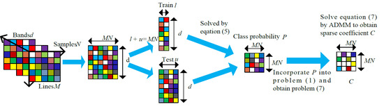
To our knowledge, each item of hyperspectral imagery data is in 3D. Before performing the SSC algorithm, each pixel can be treated as a
d-dimensional vector where
d is the number of spectral bands [
38] and the 3D HSI data
must be translated into 2D matrix. In this way, the HSI data can be denoted by a 2D matrix
, where
represents the width of the HSI data and
is on behalf of height of the HSI data. The sparse representation coefficient of HSIs can be obtained by utilizing Equation (1) of the SSC model.
is on behalf of sparse representation coefficient matrix of HSIs data. The SSC algorithm for HSIs data can be generalized in Algorithm 1.
| Algorithm 1. Sparse Subspace Clustering for HSI data |
| Input: pixel points of d dimension from n subspaces |
Step 1.Calculate sparse coefficient matrix by performing SSC model (1)
on points . |
| Step 2. Normalize the columns of
as . |
| Step 3. Build the similarity matrix according to Equation (3). |
Step4. Apply the spectral clustering to the
similarity to obtain theclustering results. |
| Output: clusters . |
The process of spectral clustering can be summarized as follows. Firstly, we can obtain the Laplacian matrix formed by where is a diagonal matrix. Then, we obtain the clustering results by applying the K-means algorithm to the normalized rows of a matrix whose columns are the bottom eigenvectors of the symmetric normalized Laplacian matrix.
4. Experiment and Analysis
In this section, we conduct a series of experiments to further assess the cluster effectiveness of the proposed algorithm for HSIs. To illustrate the better performance of our method, we compared our method with unsupervised clustering and semi-supervised clustering methods, respectively. As initially mentioned, unsupervised clustering methods included SSC [
23], SSC-S [
24], S
4C [
24], and semi-supervised clustering methods such as S
3R [
32], SSLRR [
33], and semi-supervised RobustLatLRR (SSRLRR) are used as benchmarks. Furthermore, S
3R, SSLRR and SSRLRR make full use of 30% labeled information to obtain sparse and low rank representation coefficients in the experiment. Finally, they use related sparse representation (SR) and LRR coefficients as the weight of graph and acquire clustering results by typically normalized cuts [
41]. The evaluation indicators used in this paper are user’s accuracy (UA) [
24], overall accuracy (OA) [
42], kappa coefficient (kappa) [
28], accuracy (AC) and normalized information metric (NMI) [
43], which are very popular clustering indicators.
4.1. Experimental Datasets
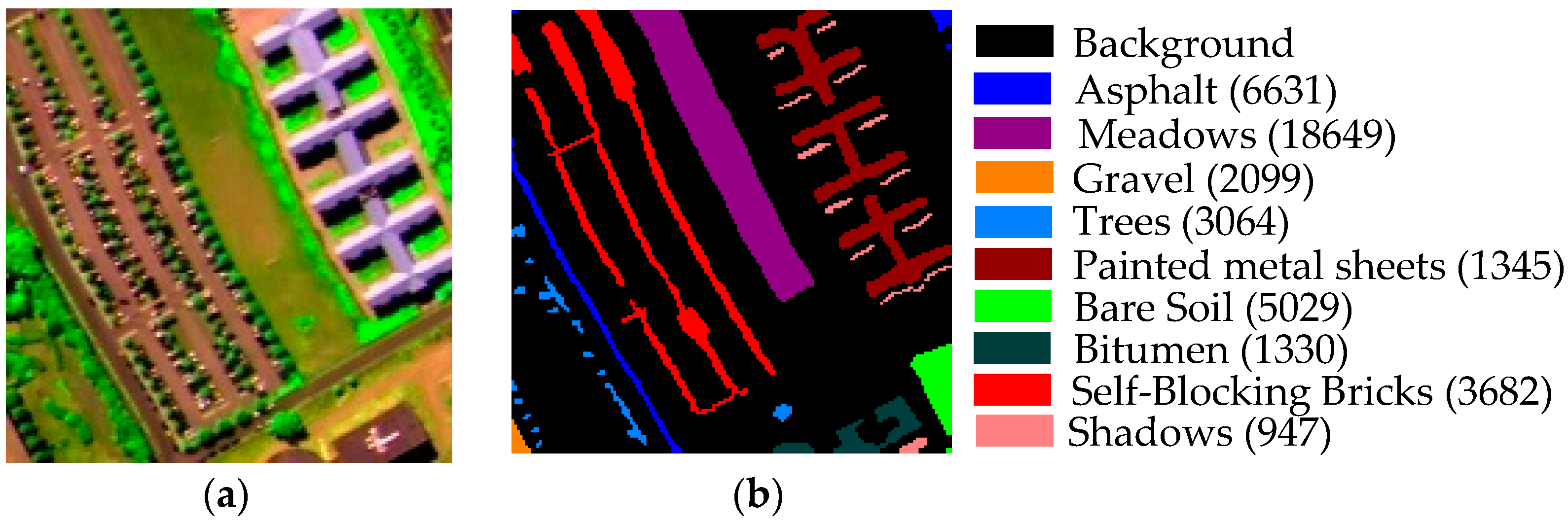
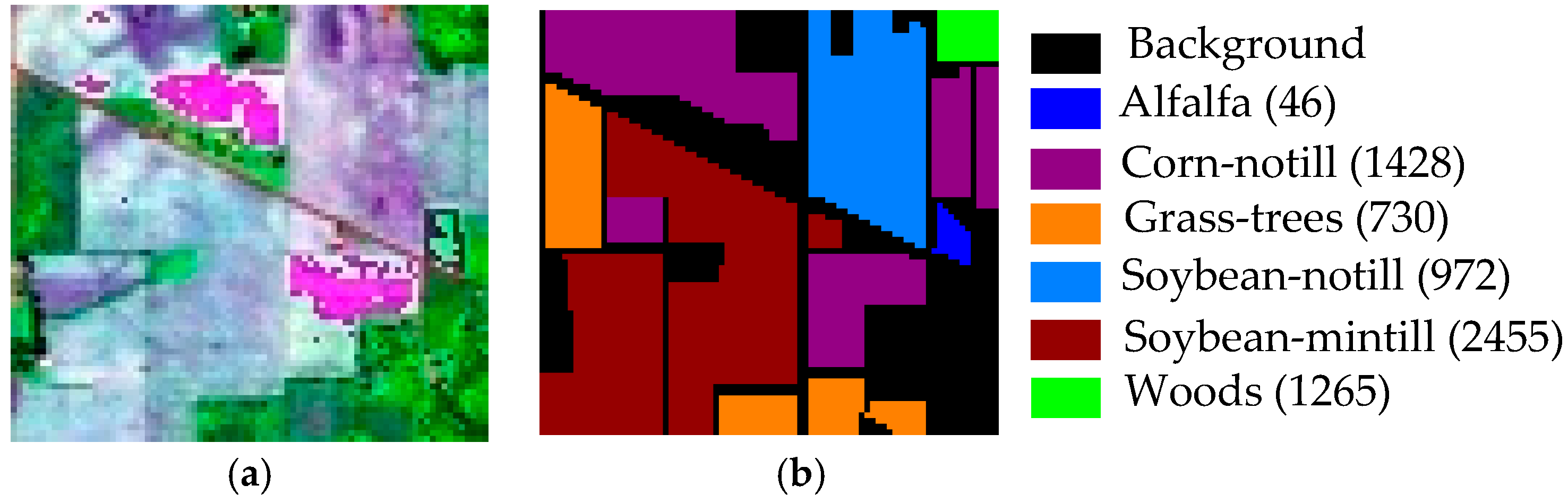
Our proposed algorithm is evaluated using two widely used hyperspectral data sets, which are the Pavia University scene and Indian Pines. The Pavia University scene is acquired by the Reflective Optics System Imaging Spectrometer (ROSIS) sensor, which has the size of
with a 1.3 m geometric resolution and has nine main classes. A typical subset of
is selected as our objective data, with nine classes. The Indian Pines data are gathered by an Airborne Visible InfraRed Imaging Spectrometer (AVIRIS) sensor with a size of
including sixteen classes, with a subset of
including six classes selected as our objective data. The false color composites and the color maps of ground truth with two scenes are shown in
Figure 2 and
Figure 3.
4.2. Experimental Procedure and Analysis
4.2.1. The Quantitative Experimental Results on the Pavia University Scene
First, we conduct our CPPSSC algorithm with 30% supervised information on the Pavia University scene data set, and the experimental cluster maps compared with these benchmarks are shown in
Figure 4.
From the visual effect of
Figure 4, we can clearly see that our algorithm, especially for such classes as the meadows, gravel and trees, demonstrates the better clustering effect and is closer to the true ground. To a certain extent, these categories obviously achieved fewer misclassifications using our algorithm. We can verify our observation from the
Table 1 and
Table 2 with quantitative experimental analysis. The bold numbers are the best clustering results.
It can be seen from
Table 1 that, according to the evaluation indicator with the UAs, the meadows, gravel and trees in our algorithm can possess the better performance compared with these benchmarks. The UAs are up to 69.77%, 30.36% and 91.15%, respectively. On the other hand, the quantitative analysis from
Table 1 confirms our visual performance. Moreover, from the UA point of view, the SSC, S
4C and SSRLRR algorithms absolutely misclassify the pixels of gravel, while the SSC-S obtains a poor accuracy of 1.79%. Apparently, their recognition effect is not satisfied. Fortunately, our CPPSSC superiorly reaches the best UA with 30.36%, which effectively exceeds the other methods and possesses the more correct pixels. The main reason is that our algorithm can deliver the supervised information to the sparse representation process, whose theoretical knowledge is similar to S
3R and SSLRR. In addition, relatively better clustering effects for asphalt and bare soil can also be acquired by our algorithm, although they are not the best ones. From
Table 2, the OA and kappa of our CPPSSC algorithm are the best compared with the other benchmarks, achieving 62.91% in OA and 0.5330 in kappa. The SSC-S and S
4C combined HSI spectral information with the wealthy spatial correlation, obtaining OAs of 48.35% and 54.87%, respectively, and also obtained kappas of 0.4037 and 0.4625 separately. It can be seen that they have a limited clustering effect for lacking known supervised information. The SSC and CPPSSC obtained OAs of 51.37% and 62.91%, and can also obtain kappa coefficients of 0.4353 and 0.5530, respectively. In other words, an CPPSSC algorithm evidently generates sharp growth, with 11.54% of OA, and achieves an improvement of 0.1177 in kappa. Compared with S
4C, our CPPSSC presents an apparent rise in OA with 8.04%, which also obtains Kappa coefficients with the distinct growth of 0.0905. This comes from the fact that our algorithm successfully utilizes the supervised information to propagate the probability about whether two samples belong to the same class and eventually deduce to intrinsic sparse representation coefficients. Although S
3R and SSRLRR can obtain better OAs at 58.14% and 58.19%, and kappas of 0.4707 and 0.4826, respectively, the CPPSSC can obtain better clustering performance via class probability structure between data samples and classes, which assists sparse representation coefficients by yielding a more discriminative diagonalization.
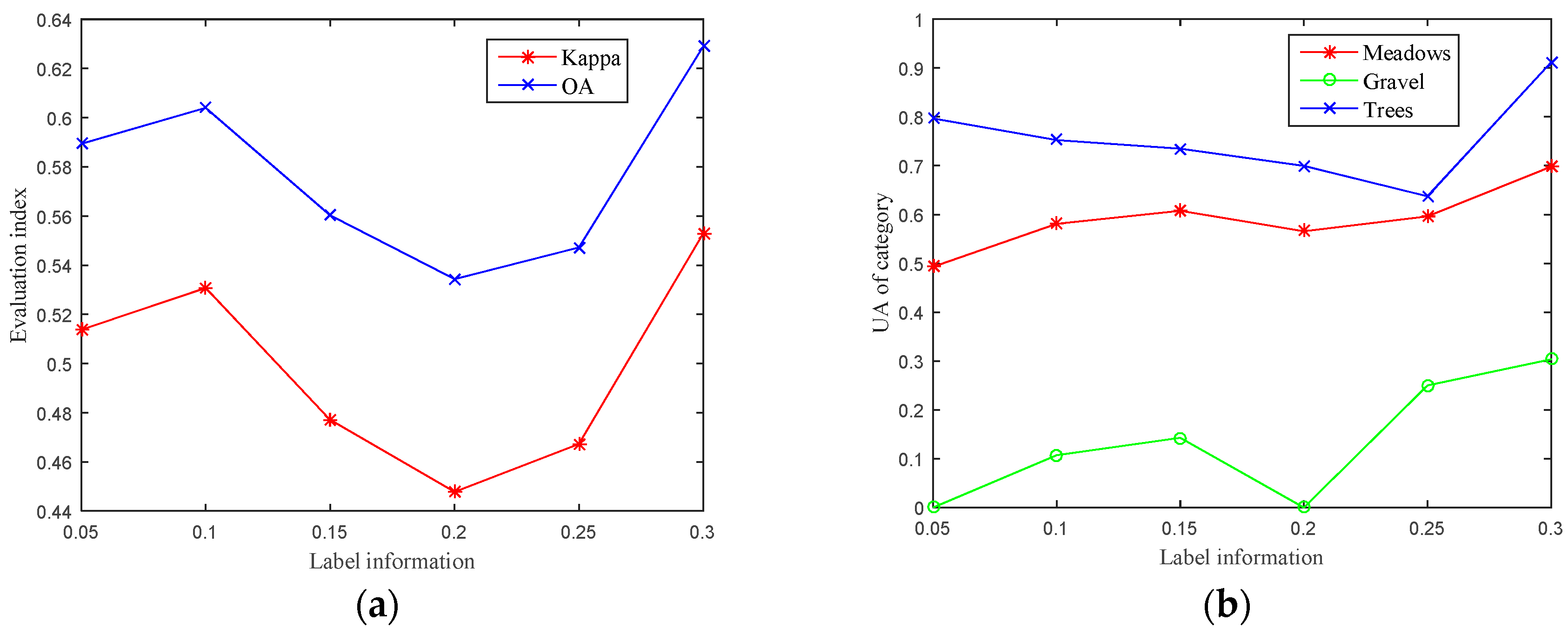
We also conduct experiment on the Pavia University scene by our CPPSSC algorithm by changing supervised information by 5%, 10%, 15%, 15%, 20% and 25%, compared with default 30% supervised information. The variation tendencies of OA s and kappas are shown in
Figure 5.
To our best knowledge, the clustering effect will be better when the supervised information accounts for a large proportion. It can be seen clearly from
Figure 5 that OA and kappa with 30% supervised information are the best compared with the other different levels of supervised information. However, the clustering results still keep fairly stable when the supervised information accounts for a proportion of 10%, which shows the low dependence of the supervised information. They also depends on other parameters such as
. The case demonstrates that our algorithm does not rely too much on supervised information. Besides, for the meadows, gravel and trees, the classification precision also can reach better clustering validity with UAs when the known class probability information can be integrated into the traditional SSC algorithm.
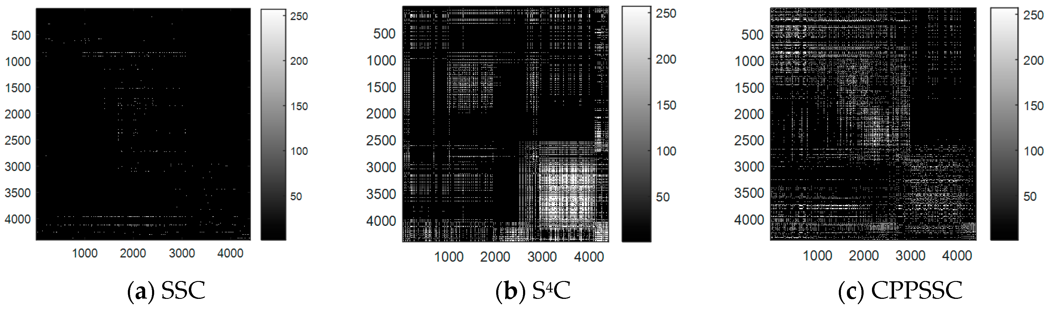
4.2.2. The Block Diagonal Structure of Sparse Coefficients
We also conduct the experiments to confirm the block diagonal structure of sparse representation coefficient with our algorithm, and the results are listed in
Figure 6.
From
Figure 6, we can see that the block diagonal structure of sparse coefficient with our CPPSSC algorithm is obviously better than with SSC and S
4C, which is in favor of self-expressiveness to boost the final clustering results. As illustrated in
Figure 6, the white spaces indicating nonzero coefficients are the block sparse coefficients among data samples. In
Figure 6a, it is difficult to form block diagonalization facing HSI data with the samples with nonzero coefficients. Although
Figure 6b can show block diagonalization to a certain extent, an imperfection is that the nonzero sparse coefficients occupy a large proportion in the overall sparse coefficient matrix, which is contrary to sparse representation theory. In terms of
Figure 6c, the block diagonalizations via our CPPSSC method are quite obvious compared with the other two methods; the reason is that the probabilistic class structure estimated the similarity between each sample and each class is incorporated into the sparse representation coefficients. Moreover, the global nonzero coefficients structure can be enhanced, which facilitate block diagonalization of sparse coefficients.
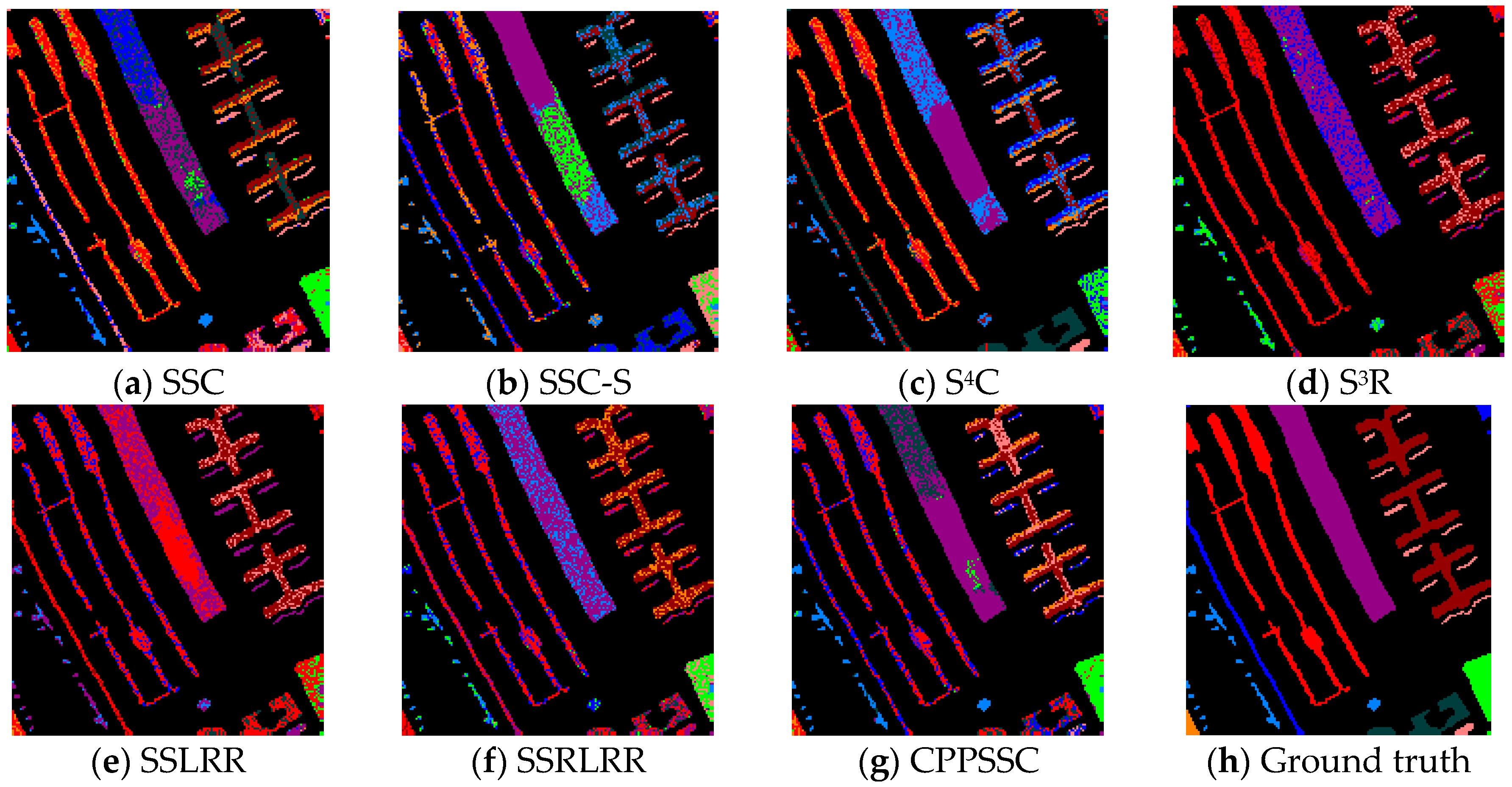
4.2.3. The Quantitative Experimental Results on the Indian Pines
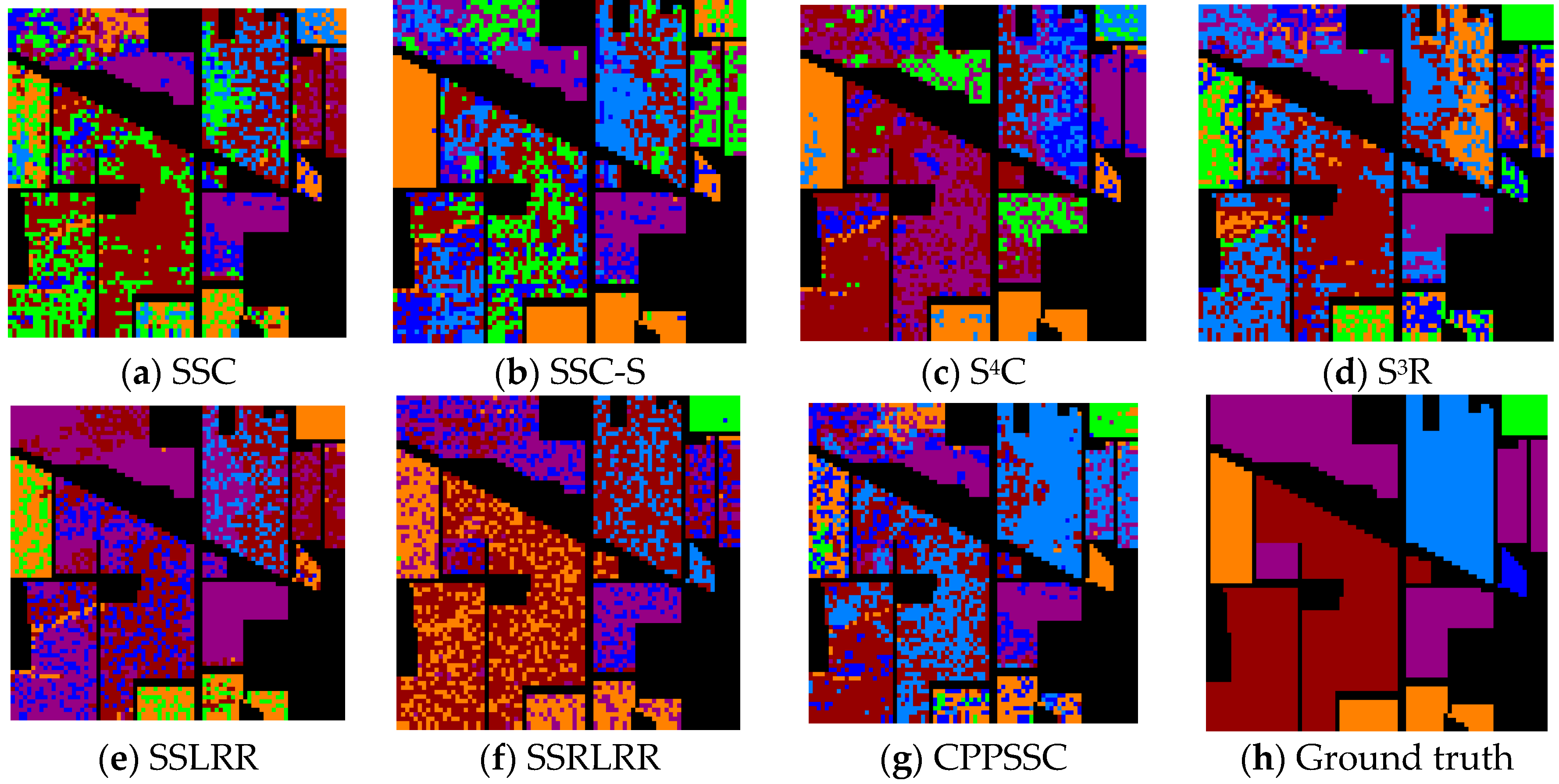
Then, we conduct our CPPSSC algorithm with supervised information of 30% on the Indian Pines data set, and the experimental effect is shown in
Figure 7.
Figure 7 shows the visual cluster maps with all kinds of clustering technologies. We can see that the visual cluster effect of the soybean-notill and woods with our CPPSSC is closer to that of the original cluster map. The quantitative data analysis is given in
Table 3 and
Table 4.
Table 3 shows the UA of every land over class, which can distinguish the clustering performance of every method. Evidently, the clustering expression of soybean-notill and woods is able to present better clustering performance via our CPPSSC, with higher UAs of 81.01% and 90.91%, respectively, reducing the misclassification. Moreover, in terms of soybean-notill, the other benchmark techniques achieve a poor UA of 30%, which is less than half that of our method. In the cluster map, the majority of soybean-notill class has been misclassified into grass-trees in SSC. At the same time, the UA of soybean-notill with the SSC-S method achieves better performance than that of SSC algorithm, with a growth of 19.81%, because of adding the spatial information into HSI clustering. However, the speed of the growth is limited. For our CPPSSC algorithm, the sparse representation can take full advantage of the known information to extract the internal essence on HSI data, which achieves the qualitative upgrade of the soybean-notill clustering. The cluster precision of the woods via our algorithm is higher, up to 90.91%. Compared with S
4C, it perfectly achieves the best clustering results for the woods class, with an improvement of almost 60% in UA. Actually, the reason for improvements in our algorithm is that signals with high correlation are preferentially selected in the sparse representation process via the spread of supervised information. The UAs of the woods in the SSC-S and S
4C, are 44.44% and 31.31%, respectively, which are far lower results than ours. The UA of woods in CPPSSC is lower than in S
3R and SSRLRR, which indirectly proves significance of supervised information for clustering.
In
Table 4, with overall precision analysis on Indian Pines, the OA and kappa values by our algorithm are the best results (presented with bold), with an OA of 58.14% and a kappa of 0.4643. The SSC-S and S
4C can obtain better cluster performance with OA precision, which is 52.13% and 54.02%. It is a fact that the two algorithms can acquire smooth growth compared with the SSC algorithm because of adding the wealthy spatial correlation of HSIs, obtaining improvements of 3.02% and 4.91% in OA, respectively. However, the promotion of the two methods has some limitations. This is because they do not utilize the known supervised information but only utilize the unknown samples to fetch information. Fortunately, our CPPSSC algorithm can rationally make full use of supervised information to spread to unknown data. Hence, our method can achieve preferable clustering precision and is more effective compared with traditional SSC algorithm, achieving an improvement of 9.03% in OA and a growth of 0.1179 in kappa. In terms of S
4C, our CPPSSC algorithm can obtain evident OA growth with 4.12%, and also obtain the kappa growth of 0.0741 by the effective class probability model. With respect to S
3R, SSLRR and SSRLRR algorithms, our CPPSSC performs better than these three methods. The reason is that our algorithm utilizes a small amount of labeled samples to generate class probability among samples, and exploits class structure information via sparse representation classification.
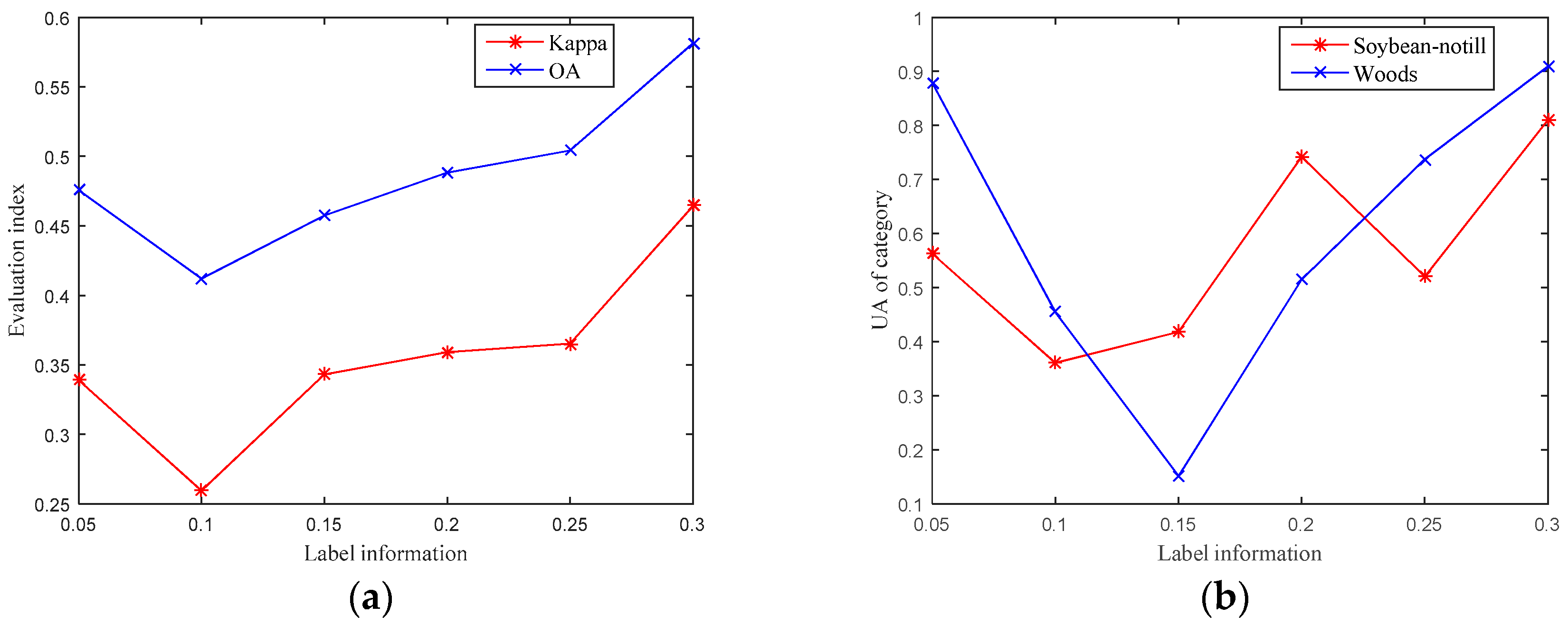
For our CPPSSC algorithm, we also carry out a series of experiments on Indian Pines with added supervised information of 5%, 10%, 15%, 20%, 25% and 30%. The experimental results are shown in
Figure 8.
In
Figure 8, the clustering precision of OA and kappa firstly shows a descending trend since the supervised information is not utilized by sparse representation process at the beginning, and then ascends because of gradually added supervised information, and it propagates to the unknown samples. In other words, we only take full advantage of the testing samples via the spare process and the reduction in the available data. Hence, the variation tendency is shown to be descending in the beginning. With the increase in supervised information, quality information can be propagated to unknown samples via class probability, and then the overall clustering accuracy will be improved. The clustering precision of Indian Pines can be best reached using 30% supervised information, with 58.14% in OA and 0.4643 in kappa. Likewise, the clustering accuracy with UA of the soybean-notill and woods can be closer to ground truth when we add the supervised information with 30% into unknown HSI sample clustering.
4.2.4. The Clustering Performance Evaluated by AC and NMI on Two Data Sets
In general, the accuracy (AC) and normalized information metric (NMI) [
43] are used to evaluate the performance of clustering method. Consequently, we have conducted experiments on the Pavia University scene and Indian Pines to verify the effectiveness of CPPSSC. The performance of the benchmarks and CPPSSC methods are listed in
Table 5.
To our knowledge, both the AC and NMI range from 0 to 1 and a higher value indicates a better result. From
Table 5, we can see that CPPSSC achieves an 3% AC gain and 6.58% NMI gain on Pavia University scene over the SSC. Besides, it is better than the other semi-supervised clustering methods. Moreover, the CPPSSC also achieves the best clustering performance over the other benchmarks on Indian Pines. The reason might be the effectiveness of the proposed class probability, which explores the relationships between the samples and class and further adds valid similarity information to SSC.
4.2.5. The Parameters Analysis in the CPPSSC Algorithm on Two Data Sets
There are two main parameters in the CPPSSC algorithm, they are and . is the tradeoff parameter between the sparsity of the coefficient and the magnitude of noise. It can be decided by the following formula.
The
is actually decided by
since
is fixed for a certain data set. Indeed, we only need to fine-tune
, and find the optimum values with OA and Kappa, which can be shown with a curve in
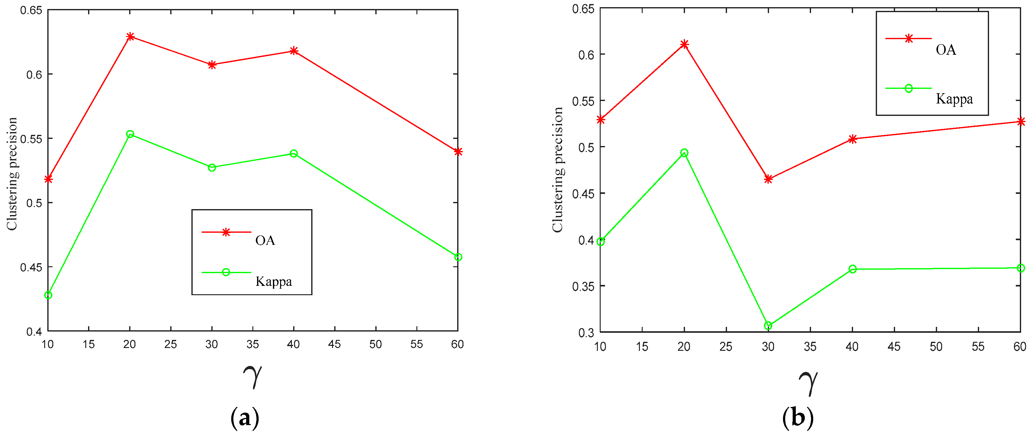
Figure 9.
The clustering precision change curves of the OA and kappa with various values of
are shown in
Figure 9. From this figure, it can be seen that the
is independent on the dataset to some extent. The optimizational values of the two data sets are located on
, which are perfectly shown on the two datasets. The OA and kappa values are respectively 0.6291 and 0.5530 on the Pavia University scene when
. In addition, the optimizational values of the OA and kappa are also achieved as0.6107 and 0.4936 when
on the Indian Pines data set. It can be seen that our CPPSSC can achieve a better clustering accuracy with
, and makes sense for HSI clustering.
To show the computation complexity of these clustering methods, we also perform the experiments on two data sets. The computational time of different clustering methods (seconds) is shown in
Table 6.
From
Table 6, we can see that SSC is fast in the Pavia University scene and Indian Pines, and CPPSSC spends the more time than SSC and SSC-S but less than the other clustering methods. The main reason is that CPPSSC has to spend a little time to estimate the class probability distribution of unlabeled samples.
4.3. Discussion
From the experimental results, we can see that, compared with the unsupervised and semi-supervised methods, our algorithm is informative and discriminative. The reason is that firstly, SRC can obtain a good estimation of the underlying class structure of test samples by utilizing a small amount of labeled samples. This is named probabilistic class structure. Then, the class probability is incorporated into the sparse representation coefficient to strength the global similarity structure among all the samples and preserve the subspace-sparse representation by facilitating the block diagonalization of sparse coefficients.
The computational complexity of the CPPSSC algorithm depends on updating and in Algorithm 3. Specifically, the computation complexity of it is about , where is the number of data samples. The computation complexity of updating , , and is . In summary, the computational complexity of CPPSSC algorithm is , where is the number of iterations.
To obtain the uniform class probability between each unlabeled sample and each specific class addressed by SRC, we prefer to use the
norm instead of the
norm to deal with
, although the
norm has been proven unimportant to classification in theory [
44] and practice [
45]. The reasons can be summarized as follows. First, in SRC, Wright et al. verified that the SRC coefficients solved by
minimization are much less sparse than by
minimization. We hope to obtain the much sparser representation of self-expressiveness of data. Second, since both the SRC and SSC are based on the
norm, this leads to a combined norm that also has the structure of the
norm. It will facilitate the block diagonal structure of sparse coefficients. The third reason to use the
norm is the greatly theoretical guarantees for correctness of SSC, which can be applicable to detect subspace even when subspaces are overlapping [
46].
A number of supervised classification methods have been suggested. Compared with supervised classification methods, the advantage of semi-unsupervised methods for HSIs can be summarized as follows. First, the supervised classification needs a great deal of labeled samples to improve the classifier performance [
47]. However HSI classification often faces the issue of limited number of labeled data, which are often costly, effortful, and time-consuming [
28]. On the other hand, we can obtain a large number of unlabeled data effortlessly. Semi-supervised learning (SSL), which can utilize both small amount of labeled instances and abundant as well as unlabeled samples, has been proposed to deal with this issue [
48]. Second, in essence, semi-supervised clustering such as using the CPPSSC method adds the constraints of a small amount of labeled information to the objective function for assigning similar samples into corresponding class. These constraints are used to estimate the similarity between data points and thereby enhance the clustering performance [
49]. Consequently, the semi-supervised clustering algorithms are becoming more popular because of the abundance of unlabeled data and the high cost of obtaining labeled data.
What should be denoted is that, to be honest, we cannot guarantee that all the UAs of corresponding classes via the CPPSSC algorithm are the best because of the different data structures of each class. The main reason is that CPPSSC algorithm has difficulty in estimate class probability of every data point because of the redundant information of complex HSI bands.


