A Self-Calibrating Runoff and Streamflow Remote Sensing Model for Ungauged Basins Using Open-Access Earth Observation Data

Abstract

Due to increasing pressures on water resources, there is a need to monitor regional water resource availability in a spatially and temporally explicit manner. However, for many parts of the world, there is insufficient data to quantify stream flow or ground water infiltration rates. We present the results of a pixel-based water balance formulation to partition rainfall into evapotranspiration, surface water runoff and potential ground water infiltration. The method leverages remote sensing derived estimates of precipitation, evapotranspiration, soil moisture, Leaf Area Index, and a single F coefficient to distinguish between runoff and storage changes. The study produced significant correlations between the remote sensing method and field based measurements of river flow in two Vietnamese river basins. For the Ca basin, we found R² values ranging from 0.88–0.97 and Nash–Sutcliffe efficiency (NSE) values varying between 0.44–0.88. The R² for the Red River varied between 0.87–0.93 and NSE values between 0.61 and 0.79. Based on these findings, we conclude that the method allows for a fast and cost-effective way to map water resource availability in basins with no gauges or monitoring infrastructure, without the need for application of sophisticated hydrological models or resource-intensive data.

1. Introduction

Due to economic and demographic development pressures, water is becoming an increasingly valuable resource [1,2]. Access to clean and affordable water is vital for drinking, sanitation, and especially food production (the dominant use of fresh water). Insight into available water resources under climatic change and intensified agricultural production systems is crucial for effective water allocation. Intensified agricultural production systems have high water requirements, whereas climate change presents a compounding threat to fresh water for human use (including agriculture, drinking and industrial), due to an increased magnitude and a higher frequency of floods and droughts [3]. While human water use is often a key priority for water resource allocation, important ecosystem services supplied by water should also not be ignored.

In countries where the water resources are under the most pressure, data on water availability and usage is often scarce [4]. Therefore, open access global-scale water-related data products derived from remote sensing have found their way into many studies in the field of hydrology to investigate water resource availability [5,6,7]. In addition, frameworks to support stakeholders in planning water resources, such as Water Accounting+ (WA+), use these data products to estimate spatio-temporal distribution of water resources [8,9]. Satellite-derived data products on precipitation, evapotranspiration, soil moisture and Leaf Area Index have a strong physical foundation, are well-tested and have a good overall accuracy [10]. However, information on river flow and groundwater storage changes are also required in order to calculate all terms of the water balance. These data are often difficult to acquire, and, when available, often are of a poor quality, contain gaps or have errors. Complex hydrology models are frequently applied to fill these gaps, but these models also require a large amount of physical data that is not readily available [11]. Although this has increasingly prompted the scientific community to use satellite-derived data as model input, an established, fully satellite-based approach for pixel-based evaluation of the water balance is not yet available.

In this manuscript, we present a formulation to estimate surface runoff and storage changes in ungauged basins. This innovative method solely relies on freely available global remote sensing products. The demonstrated approach can have a wide range of applications, as it does not require the implementation of complex hydrology models or a large number of physical parameters. As such, river flow and storage changes can be calculated without ancillary data. The work is presented in the context of the trans-boundary Ca River basin in Vietnam. Like many other river basins in southeast Asia [12,13], there are many water related problems in the Ca River basin due to water shortage, pollution, and competing interests. In addition to this, the Ca River basin has recently experienced a drought and salt water intrusion, making it the focal point for a USAID funded study on alternative water resource management strategies. However, data scarcity hampers a comprehensive insight into available water resources. As such, we selected the Ca basin as an example to test the applicability of our streamflow remote sensing model.

2. Materials and Methods

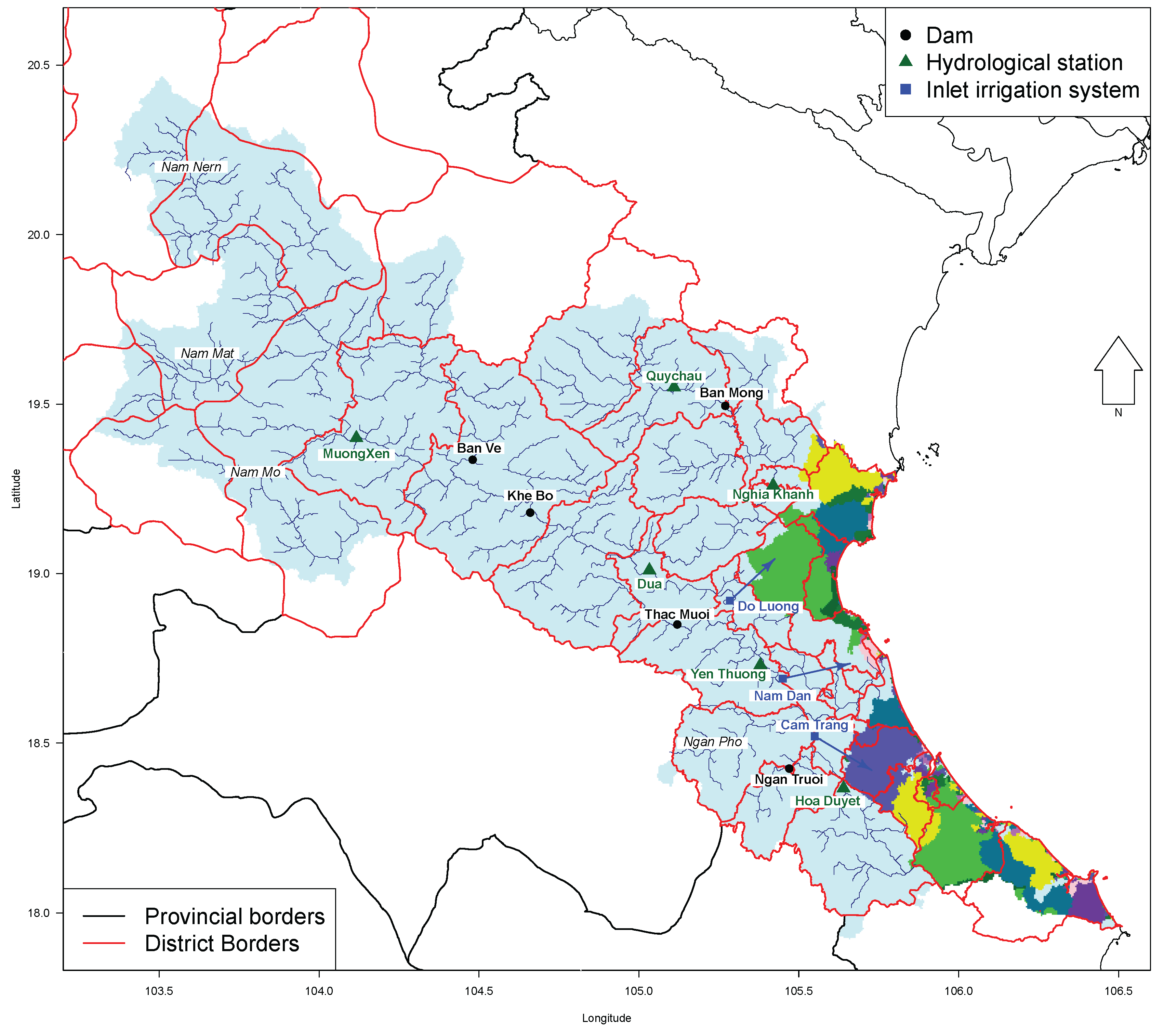
2.1. Study Area

The Ca River Basin (Figure 1) is located in the North-Central region of Vietnam. The river basin covers an area of approximately 27,000 km² (Figure 1). About 65% of the total territory of the trans-boundary river system is located in Vietnam and the rest is in the Lao People’s Democratic Republic (LPDR). The upstream northwestern part of the basin consists of highlands with elevations ranging from 1000–2600 m, located in the Huaphahn and Xiangkhouang of the LPDR. The eastern part of the basin covers part of the Vietnamese provinces of Nghe An and Ha Tinh. More then four million people reside in the basin and about 20% of the total area is used for agricultural purposes. Three large irrigation systems transport water from the Ca basin to smaller basins that are hydrologically not part of the Ca basin. Five larger dams were recently constructed in the basin with a gross capacity ranging between 97.8 and 1834.6 mm³. Monthly river flow data was collected for six stations for the period 2000–2010.

2.2. Climatic Setting

Vietnam has a tropical monsoon type climate that is influenced by two distinct rainfall regimes [14]. Summers are dominated by the the South Asian monsoon, which begins in early May in the southern part of Vietnam and moves northward until late July–August. Precipitation amounts in the rainy season, which starts in May and ends in October are related to the migration of the monsoon over the continent. Due to Vietnam’s geographic stretch from North to South, months with peak amounts of precipitation vary between provinces [15]. Winters are dominated by the East Asian monsoon. This monsoon is cold and dry and mainly impacts the North and Central Areas of Vietnam [15]. The Northern part of Vietnam receives the most precipitation in the summer, whereas the central part is characterized by a fall regime. Inter-annual variations in precipitation are linked with changes in the El Nino–South Oscillation [16,17].

2.3. Input Products

In this study, we used remote sensing derived data on precipitation (0.05°), evapotranspiration (0.0025°) and soil moisture (0.005°). Furthermore, data on canopy interception were derived. All data have the monthly time resolution. These data were used in water balance calculations.

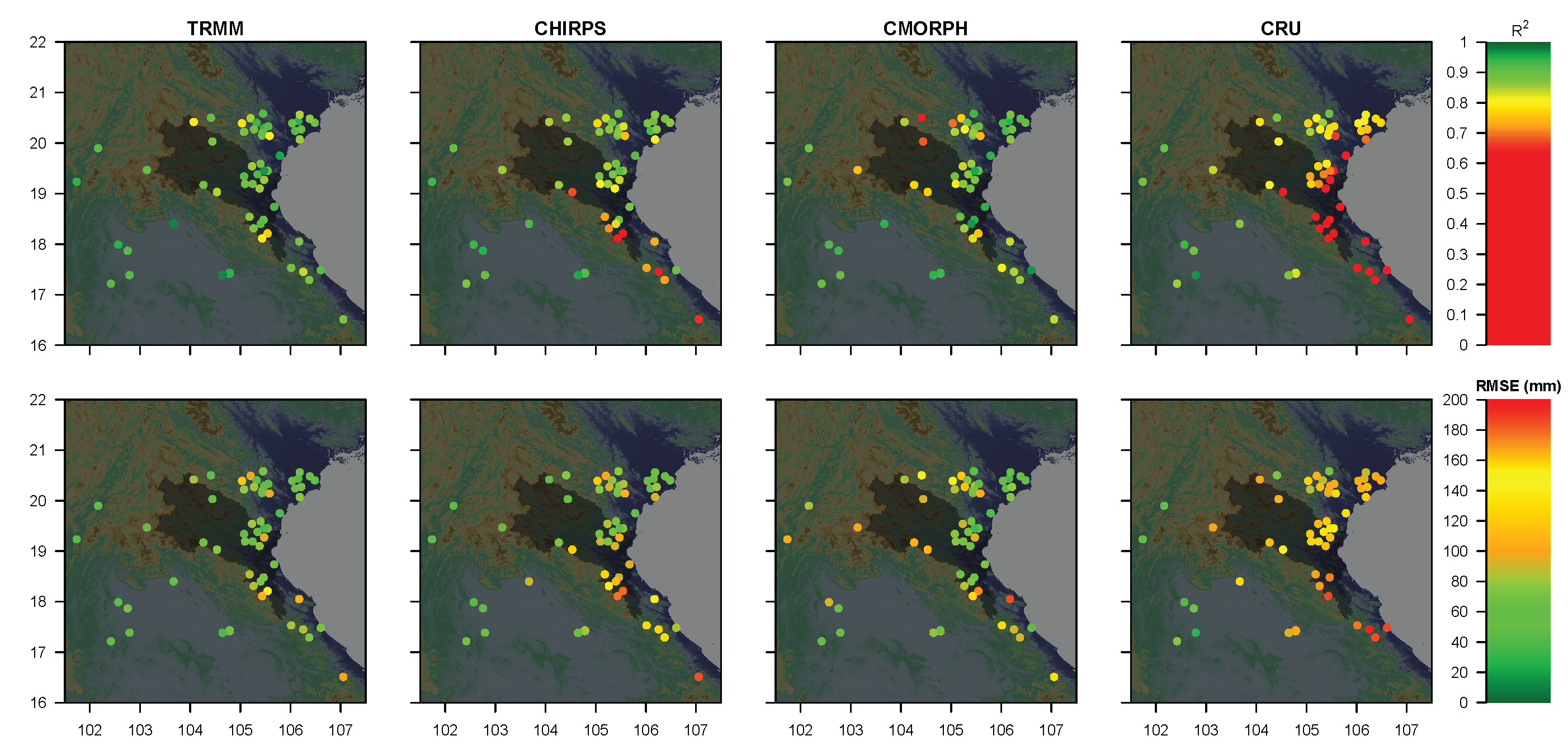
2.3.1. Precipitation

Four gridded precipitation products were compared with data from rain gauges to validate the consistency between ground measurements and the precipitation products. A total of 59 rainfall gauges were included in the analysis. Physical data records were obtained from [18] and the National Oceanic and Atmospheric Administration’s (NOAA’s) National Climatic Data Center (NCDC; [19]). Due to the limited coverage of measurement stations within the Ca basin, the extent of the study area was widened to increase the number of points at varying elevations. Four different global monthly precipitation products were compared with the in situ measurements. The products were obtained from different sources for the period 2001–2010, the temporal coverage of the in situ data. Products from the Tropical Rainfall Measurement Mission (TRMM) and the Climate Hazards Group InfraRed Precipitation Station (CHIRPS), the Climate Prediction Center Morphing Technique (CMORPH) and the Climate Research Unit at the University of East Anglia (CRU; ts 3.22) were used.

Table 1. Institutional rainfall products.

Abbreviation	Product	Institute
TRMM	Tropical Rainfall Measurement Mission	NASA
CHIRPS	Climate Hazards Group InfraRed Precipitation Station	Climate Hazards Group
CMORPH	Climate Prediction Center Morphing Technique	NOAA /CPC
CRU	Climate Research Unit	University of East Anglia

provides an overview of the different products and institutes involved in creating these data.

The rainfall products have different origins and apply various methodologies to estimate the monthly precipitation (

Table 2. Rainfall products methods and spatial resolutions. See Table 1 for details.

Abbreviation	Method	Resolution
TRMM (3B43)	Microwave (TMI, SSMI, AMSU and AMSR)	0.25°
	Infrared (GMS), Gauge data
CHIRPS	CHPClim, Infrared & Microwave (TRMM (3B43)	0.05°
	CFSv2. Gauge data
CMORPH	Microwave estimates (DMSP F-13, 1415 (SSM/I)	0.25°
	NOAA-15, 16, 17 & 18
	(AMSU-B), AMSR-E, and TRMM TMI
	IR motion vectors, Gauge data
CRU	Surface station observations	0.50°

). The TRMM (3B43) data is constructed from a C-band radar and passive microwave sensors designed to obtain quantitative information on rainfall including infrared measurements from both TRMM sensors as well as from geostationary meteorological satellites (GMS). TRMM has a resolution of 0.25°. CHIRPS has the highest spatial resolution (0.05°) and is an ensemble product based on various interpolation schemes using a variety of sources such as monthly precipitation climatology (CHPClim) satellite measurements, atmospheric model rainfall fields (CFSv2) and surface measurements [20]. CMORPH has similar inputs as TRMM, but uses the motion vector derived from stationary IR satellite data to interpolate precipitation at times that passive microwave data is not available [21]. CRU is constructed from surface station observation and has a resolution of 0.5° [22].

Figure 2 shows the R² (top) and Root Mean Square Error (RMSE) (bottom) for all stations using the TRMM, CHIRPS, CMORPH and CRU datasets (from left to right). A generally good agreement was found, considering common problems in terms of scale mismatch between single point rain gauge measurements and satellite derived integrated rainfall measurements (e.g., [23,24]). TRMM performs best in terms of R² and RMSE, followed by CHIRPS and CMORPH. The latter performs relatively well in lowlands, but has poor performance in the highlands. The performance of CRU is generally poor.

The TRMM and CHIRPS data were combined into an ensemble product, as TRMM shows the best performance with a relatively coarse spatial resolution while CHIRPS shows acceptable performance with a higher spatial resolution. The ensemble product was created by downscaling the TRMM to a 0.05° resolution using the pixel distribution of CHIRPS. The total precipitation in one TRMM pixel was distributed over a higher density grid using the CHIRPS data of that same area. Finally, the downscaled TRMM grid and CHIRPS data were averaged as the combined product was found to give more consistent results. A comparison between the monthly averaged measured and estimated precipitation using the ensemble grid is shown in Figure 3. It can be seen that there is a good agreement between the measured and estimated total monthly precipitation(R² = 0.98, p < 0.001). While satellite derived precipitation products have limitations in terms of accuracy and resolution for extreme rainfall events [25], it has been demonstrated that they produce reliable data on longer spatio-temporal scales.

2.3.2. Evapotranspiration

Evapotranspiration (refered to as ET hereafter) is an important process in the hydrological cycle, as it accounts for a large portion of the total water outflow from the basin. ET includes evaporation from the soil, water bodies, vegetated surfaces and transpiration from plants. In contrast to precipitation, it is difficult to obtain data on ET. Whereas rain gauges and satellite derived precipitation products are commonly available, data on ET is often scarce, while its spatial and temporal variability can be large. However, methods to estimate ET from space born data using the surface energy balance haven been improved in the last decades, resulting in global scale data products. A review of [10] states that remote sensing techniques offer spatially dense estimates of the actual ET with an overall accuracy estimated at 95%.

The operational Simplified Surface Energy Balance (SSEBop) was used in this study. SSEBop is a global application of the Simplified Surface Energy Balance approach (SSEB [26]), which was mainly focused on small scale irrigation systems. The global scale approach contains a new parametrization using predefined boundary conditions for hot and cold reference conditions on a pixel scale [26]. SSEBop was successfully tested in in the semi-arid Plains using Landsat data and lysimeteric observations [27], and was tested recently against 20 flux towers scattered across USA [28]. SSEBop performed well in water balance analyses of the Nile [5] and Red River basins [6].

Since there were no in situ measurements available to validate SSEBop, the SSEBop product was linked to precipitation and reference evaporation from the Global Land Data Assimilation System (GLDAS) product in the Budyko curve in order to evaluate the performance. The ratio of ET to P was plotted as function of the ratio of reference evaporation (ET_p) to P, also known as the aridity index or Budyko curve [29]. Equation (1) shows the original formulation of Budyko, where $\varphi$ is defined as the aridity index ET_p/P. ET_p was obtained from GLDAS [30]. Actual ET retrieved from SSEBop should be in line with the theoretical work of Budyko

$$\frac{E_a}{E_p}={\left[\varphi tanh(\frac{1}{\varphi })(1-{exp}^{-\varphi }\right]}^{0.5}.$$

(1)

The relation among actual ET, reference evaporation and rainfall of the dataseries is shown in Figure 4, where a higher density of points is represented by a higher intensity color. It can be seen that the highest density of points is located close to the the original formulation [29,31] or in the ±10% range, indicated with dashed lines. The results show that the SEBBop product gives estimates on actual ET that are in close agreement with theory.

2.4. Interception

Rainfall interception by canopy cover can be an important process in the water balance, as a portion of the intercepted water is directly evaporated and can not be used by surface runoff and vegetation for transpiration. The Leaf Area Index (LAI) was calculated from the Enhanced Vegetation Index (EVI) to estimate ground area covered by vegetation [32].

The amount of intercepted rainfall (I; in mm) was calculated by Equation (2) [33,34] using the LAI (Equation (3)), P (mm·day⁻¹) and an empirical coefficient (a; mm·day⁻¹) representing the maximum water film that can be stored on a leaf. The canopy cover is determined from the Normalized Difference Vegetation Index (NDVI) using Equation (4). For empirical parameter a, we assumed a = 1 (mm·day⁻¹). The $NDV{I}_{max}$ and $NDV{I}_{min}$ represent the maximum and minimum NDVI, respectively. Daily rainfall was calculated from the remote-sensing derived P and the number of rainy days each month. The latter was calculated from the meteorological data.

$$I=a\times LAI\times \left(1-\frac{1}{1+\frac{1+cc\times p}{a\times LAI}}\right),$$

(2)

$$LAI=(3.618\times EVI-0.118)>0,$$

(3)

$$cc=1-{\left(\frac{NDV{I}_{max}-NDVI}{NDV{I}_{max}-NDV{I}_{min}}\right)}^c.$$

(4)

2.4.1. Soil Water and Groundwater

Groundwater plays an important role in catchment hydrology. Despite advances in deriving groundwater estimations from gravimetric measurements [35,36], it remains difficult to estimate catchment scale groundwater quantities. However, the amount of water stored in the upper layer of the soil can be estimated by means of remote sensing [37]. The Advanced Scatterometer (ASCAT) is an active microwave remote sensing instrument designed to monitor winds over the oceans, but also used for soil moisture purposes [38,39,40]. In order to obtain information of the root-zone rather than only the top-layer, we use the the Soil Water Index (SWI; m³·m⁻³; [41]). This product provides soil moisture estimates in relative units ranging between wilting level and full saturation. The product applies an exponential filter to estimate soil moisture in the deeper layers [38,42]. The product provides a series of 10 daily soil moisture estimates using a different time integration for each image, where longer time windows provide better estimates for deeper soil layers [43]. To gain insight into water resources in the soil layer, data products derived from a time length of 60 days were aggregated into monthly maps. The monthly soil water amount ($s{w}_m$; m) was estimated from the maximum available soil moisture, and SWI (Equation (5)). $s{w}_{max}$ was calculated from the depth of the soil layer ($Z_r$; m) and the available water content ($W{C}_{avail}$; m³·m⁻³), which represents the available water content between field capacity and wilting point. Maps of $W{C}_{avail}$ content were obtained from [44], who applied pedotransfer functions to derive soil hydraulic properties from the freely available global SoilGrids 1 km dataset ([45])

$$s{w}_m=SWI\times s{w}_{max},$$

(5)

$$s{w}_{max}=Z_r\times W{C}_{avail}.$$

(6)

Whereas the rainfall was available with 5 km pixels, ET and LAI were available at 30 m Landsat pixel scale. Such level of detail could also be worked out for soil moisture mapping (e.g., [46]), and rainfall downscaling techniques are also under development (e.g., [47]). The latter implies that the equations presented could be used to predict an unprecedented high resolution runoff processes.

2.5. The Water Balance Model

The method presented relies on the water balance (Equation (7)) using the conservation of mass principles in a soil column with defined depth. In the absence of additional supplies from river inflow, flooding and irrigation, monthly precipitation ($P_m$) equals the monthly runoff ($R_m$; mm), evapotranspiration ($E{T}_m$; mm) and storage changes ($\Delta S_m$; mm). Monthly storage changes were calculated as $S_m-S_{m-1}$

$$P_m=R_m+E{T}_m+\Delta S_m.$$

(7)

The storage component was separated into two compartments (Equation (8)), the water available in the root zone, referred to as the soil water component $S{W}_m$ and a groundwater component $G{W}_m$. The storage change was calculated as the sum of the two.

$$\Delta S_m=\Delta G{W}_m+\Delta S{W}_m.$$

(8)

The pixel-wise surface runoff ($R_m$; mm) was calculated with Equation (9) ([48,49]). It contains two components: the monthly flux of water incident on the soil surface including precipitation and interception ($I_m$; mm) ($P_m-I_m$) and root zone moisture deficit ($S{W}_{max}-S{W}_m$; mm). The maximum available soil moisture is represented by $S{W}_{max}$ (mm)

$$R_m=\frac{{(P_m-I_m)}^2}{P_m-I_m+s{w}_{max}-s{w}_m}.$$

(9)

While $R_m$ might give accurate results on a small scale, it is not suitable for application in larger areas as no storage component or retention time is included in the formula. Therefore, we attribute a fraction of the total runoff to storage changes, as shown in Equation (10), where Equations (7) and (9) are combined

$$P_m-E{T}_m=F\times \frac{{(P_m-I_m)}^2}{P_m-I_m+s{w}_{max}-sw}+(1-F)\times \Delta S_m.$$

(10)

Equation (9) and the left term of Equation (10) can be solved by remote sensing data. However, storage changes include changes in $G{W}_m$ and $S{W}_m$. Soil moisture can be estimated from microwave or thermal infrared measurements [37]. As $S{W}_m$ can be estimated from soil moisture maps, Equation (11) was used to close the water balance. Here, Δ$G{W}_m$ is calculated from the runoff (Equation (12)), assuming that a portion of the total runoff is comprised of slow groundwater runoff. We added factor F to the equation, which was used as a calibration parameter to make sure the amount of P-ET matches the runoff and storage changes on a basin scale over the whole period for the catchment. As ΔS should be expected to be 0 over the whole period, F is in fact used to scale the runoff with P-ET, while changes in storage should result in a better temporal alignment. Hence, it can be concluded that F can be calibrated without ancillary data, as all parameters in Equation (11) are deduced from remote sensing derived products

$$P_m-E{T}_m=F\times \frac{{(P_m-I_m)}^2}{P_m-I_m+s{w}_{max}-sw}+\Delta S{W}_m+\Delta G{W}_m,$$

(11)

where

$$\Delta G{W}_m=(1-F)\ast (R_m-R_{m-1}).$$

(12)

The monthly river flow was calculated for different gauging stations in the basin. The monthly flow was calculated as the sum of the upstream area using the direct runoff (R_m) and storage changes ΔS_m (Equation (13)). Negative changes in ΔS_m result in higher river levels, whereas positive changes result in lower direct runoff

$$Q_m=\sum R_m-\Delta S_m.$$

(13)

3. Results

The presented method produces significant and operational results for water resource managers, as you can see in Figure 5. An internal calibration of the water balance was created by calculating R_m = P − ET for all soil depths (Z_r; Equation (6)) between 0 and 2 m (Equation (11)) for the whole period, resulting in no need for ground data. This internal calibration method is dynamic as seen in Figure 5 that shows F for a range of Z_r, including the R² and Nash–Sutcliffe efficiency measure (NSE) [50] for monthly P_m − ET_m versus monthly R_m + ΔS_m and measured versus estimated river flow. In this example, we used the Dua gauging stations, as this station has the best match in terms of multiyear water balance, while it covers a large portion of the basin (see Figure 1). NSE and R² values for simulated and measured river flow were calculated by comparison of the monthly median flow quantities. It was found that F values vary between 0.44 and 1 and that R² for P_m − ET_m and R_m + ΔS_m is high (>0.94) for all depths. The NSE is rather low for smaller depths but increases for greater depths. Both R² and NSE show an optimum depth (m) around 0.4–0.5 m for river discharge for the Ca sub-basin.

Distributions in monthly simulated river flow were compared with the measured ones using a depth of 0.5 m. Figure 6 shows the results for six gauging stations in the basin, where the R² and NSE were calculated from the medians. It can be seen that there is good overall performance in terms of temporal distribution as well as quantity. The R² values range from 0.88 for Hoa Duyet and 0.97 for Dua and Nghia Khanh and were all found to be significant (p < 0.001). The lowest NSE was found for Hoa Duyet (0.44) and the highest (0.88) for Dua and Nghia Khanh. However, the estimated upper quantiles are lower than the measured ones. For Muong Xen and Quy Chau, there is a general underestimation of flow quantity.

To test whether the model can be applied universally, it was also applied to the Red River basin in China and Vietnam. Data from the study of Simons et al. [6] was used to run the model, and more details can be found in their study. Figure 7 shows that an optimum depth of 0.8 m was found with an F value of 0.68 (top right corner) using the most downstream station (Son Tay) to close the multi-year water balance. The results were compared with six river flow stations (left and right images). Overall, there is good agreement between simulated and measured river flows. The R² varies between 0.87 for Vu Quang and 0.93 for Yen Bai and Son Tay. The lowest NSE value was found for Vu Quang (0.61), and the highest for Son Tay (0.79). Systematic differences between measured and estimated Q could at least partly be ascribed to factors such as reservoir operations and interbasin groundwater flows, as discussed in detail by Simons et al. [6].

4. Discussion

We have shown that our formulation can be used to quickly solve all terms in the monthly water balance using only data retrieved from remote sensing, and that the model calibrates itself. On the monthly scale, the performance of this satellite-based approach rivals that of more complex and data-intensive hydrological models. NSE values on the order of 0.6–0.8, such as those observed in this study, are generally considered high in the context of hydrological model applications [51]. The application of a pixel-based approach, integrating various sources of open-access satellite data to evaluate the full water balance, is rather unique. Whereas many models such as Soil and Water Assessment Tool (SWAT) [52], Spatial Tools for River Basins and Environment and Analysis of Management Options (STREAM) [53,54], Spatial Processes in Hydrology (SPHY) [55] and PCRaster Global Water Balance (PCR-GLOBWB) [56,57] can ingest remote sensing products while performing calculations on a gridded landscape, they do not calculate the soil water balance for each pixel solely from satellite imagery. In comparison to many other hydrology models, it should be noted that the applicability of the demonstrated approach is restricted to temporal resolutions of months to years. For applications such as flood modeling, hourly to daily time steps are required, and advanced hydrological models provide substantial added value.

Another limitation of the proposed method is that additional supplies of water are not included in the analysis. Man-made interventions in the natural water cycle such as irrigation schemes and hydraulic infrastructure are disregarded. Large-scale redistribution of water resources is visible from space, and thus included in ET and SWI estimates, but is lacking on the supply side of the water balance equation. In addition, a prerequisite of the method to generate reliable outcomes is that estimates on P, ET and SWI are sufficiently accurate. We did an extensive validation of the precipitation products but had no field data for ET and SWI. In addition, simple linear relationships used in this study to e.g., link EVI with LAI (Equation (3)) can be further refined. There are a large number of different products on P and ET, all developed in their own specific geographic domains. As such, it is necessary to evaluate the suitability for the area under consideration. Techniques for doing so are well-described in [23,58,59,60], among others. Reliable field data of one gauging station in the basin is helpful to determine the optimum depth (z_r) in relation to coefficient F.

5. Conclusions

Available global remote sensing derived data products offer great opportunities to study water resource availability. We have demonstrated that these products can be integrated to solve a typical water balance equation without the need for complex and resource intensive ancillary data. This method provides a rapid, accurate, and cost-effective solution to mapping water resource availability in basins with no gauges or monitoring infrastructure, one that can be used by water resource managers to make informed decisions in a changing climate and with increasing demands on limited water supplies.

References

1. Rijsberman, F.R. Water scarcity: Fact or fiction? Agric. Water Manag. 2006, 80, 5–22. [Google Scholar] [CrossRef]
2. Mekonnen, M.M.; Hoekstra, A.Y. Four billion people facing severe water scarcity. Sci. Adv. 2016, 2. [Google Scholar] [CrossRef] [PubMed]
3. Tolentino, P.L.M.; Poortinga, A.; Kanamaru, H.; Keesstra, S.; Maroulis, J.; David, C.P.C.; Ritsema, C.J. Projected Impact of Climate Change on Hydrological Regimes in the Philippines. PLoS ONE 2016, 11. [Google Scholar] [CrossRef] [PubMed]
4. Lakshmi, V. The role of satellite remote sensing in the prediction of ungauged basins. Hydrol. Process. 2004, 18, 1029–1034. [Google Scholar] [CrossRef]
5. Bastiaanssen, W.G.; Karimi, P.; Rebelo, L.M.; Duan, Z.; Senay, G.; Muthuwatte, L.; Smakhtin, V. Earth observation based assessment of the water production and water consumption of Nile Basin agro-ecosystems. Remote Sens. 2014, 6, 10306–10334. [Google Scholar] [CrossRef]
6. Simons, G.; Bastiaanssen, W.; Ngô, L.A.; Hain, C.R.; Anderson, M.; Senay, G. Integrating Global Satellite-Derived Data Products as a Pre-Analysis for Hydrological Modelling Studies: A Case Study for the Red River Basin. Remote Sens. 2016, 8, 279. [Google Scholar] [CrossRef]
7. Karimi, P.; Bastiaanssen, W.; Sood, A.; Hoogeveen, J.; Peiser, L.; Bastidas Obando, E.; Dost, R. Spatial evapotranspiration, rainfall and land use data in water accounting. Part 2: Reliability of water accounting results for policy decisions in the Awash basin. Hydrol. Earth Syst. Sci. 2015, 19, 533–550. [Google Scholar] [CrossRef]
8. Karimi, P.; Bastiaanssen, W.; Molden, D. Water Accounting Plus (WA+)—A water accounting procedure for complex river basins based on satellite measurements. Hydrol. Earth Syst. Sci. 2013, 17, 2459–2472. [Google Scholar] [CrossRef]
9. Molden, D.; Sakthivadivel, R. Water accounting to assess use and productivity of water. Int. J. Water Resour. Dev. 1999, 15, 55–71. [Google Scholar] [CrossRef]
10. Karimi, P.; Bastiaanssen, W. Spatial evapotranspiration, rainfall and land use data in water accounting. Part 1: Review of the accuracy of the remote sensing data. Hydrol. Earth Syst. Sci. 2015, 19, 507–532. [Google Scholar] [CrossRef]
11. Immerzeel, W.; Droogers, P. Calibration of a distributed hydrological model based on satellite evapotranspiration. J. Hydrol. 2008, 349, 411–424. [Google Scholar] [CrossRef]
12. Bui, Y.T.; Orange, D.; Visser, S.; Hoanh, C.T.; Laissus, M.; Poortinga, A.; Tran, D.T.; Stroosnijder, L. Lumped surface and sub-surface runoff for erosion modeling within a small hilly watershed in northern Vietnam. Hydrol. Process. 2014, 28, 2961–2974. [Google Scholar] [CrossRef]
13. Valentin, C.; Agus, F.; Alamban, R.; Boosaner, A.; Bricquet, J.P.; Chaplot, V.; De Guzman, T.; De Rouw, A.; Janeau, J.L.; Orange, D.; et al. Runoff and sediment losses from 27 upland catchments in Southeast Asia: Impact of rapid land use changes and conservation practices. Agric. Ecosyst. Environ. 2008, 128, 225–238. [Google Scholar] [CrossRef]
14. Cheang, B.K. Short-and Long-Range Monsoon Prediction in Southeast Asia; Malaysia Meteoorlogical Service: Petaling Jaya, Malaysia, 1987.
15. Nguyen, D.Q.; Renwick, J.; McGregor, J. Variations of surface temperature and rainfall in Vietnam from 1971 to 2010. Int. J. Climatol. 2014, 34, 249–264. [Google Scholar] [CrossRef]
16. Yen, M.C.; Chen, T.C.; Hu, H.L.; Tzeng, R.Y.; Dinh, D.T.; Nguyen, T.T.T.; Wong, C.J. Interannual variation of the fall rainfall in Central Vietnam. J. Meteorol. Soc. Jpn. 2011, 89, 193–204. [Google Scholar] [CrossRef]
17. Nguyen, T.D.; Uvo, C.; Rosbjerg, D. Relationship between the tropical Pacific and Indian Ocean sea-surface temperature and monthly precipitation over the central highlands, Vietnam. J. Meteorol. Soc. Jpn. 2007, 27, 1439–1454. [Google Scholar] [CrossRef]
18. Thomas, T.; Christiaensen, L.; Do, Q.T.; Trung, L.D. Natural Disasters and Household Welfare: Evidence from Vietnam; World Bank Policy Research Working Paper Series; World Bank: Washington, DC, USA, 2010. [Google Scholar]
19. NCDC. Available online: http://land.copernicus.vgt.vito.be (accessed on 16 January 2016).
20. Funk, C.C.; Peterson, P.J.; Landsfeld, M.F.; Pedreros, D.H.; Verdin, J.P.; Rowland, J.D.; Romero, B.E.; Husak, G.J.; Michaelsen, J.C.; Verdin, A.P. A Quasi-Global Precipitation Time Series for Drought Monitoring; US Geological Survey Data Series: Reston, VA, USA, 2013; Volume 832.
21. Joyce, R.J.; Janowiak, J.E.; Arkin, P.A.; Xie, P. CMORPH: A method that produces global precipitation estimates from passive microwave and infrared data at high spatial and temporal resolution. J. Hydrometeorol. 2004, 5, 487–503. [Google Scholar] [CrossRef]
22. Harris, I.; Jones, P.; Osborn, T.; Lister, D. Updated high-resolution grids of monthly climatic observations—The CRU TS3. 10 Dataset. Int. J. Climatol. 2014, 34, 623–642. [Google Scholar] [CrossRef] [Green Version]
23. Vernimmen, R.R.E.; Hooijer, A.; Mamenun; Aldrian, E.; van Dijk, A.I.J.M. Evaluation and bias correction of satellite rainfall data for drought monitoring in Indonesia. Hydrol. Earth Syst. Sci. 2012, 16, 133–146. [Google Scholar] [CrossRef] [Green Version]
24. Cheema, M.J.M.; Bastiaanssen, W.G. Local calibration of remotely sensed rainfall from the TRMM satellite for different periods and spatial scales in the Indus Basin. Int. J. Remote Sens. 2012, 33, 2603–2627. [Google Scholar] [CrossRef]
25. Huang, Y.; Chen, S.; Cao, Q.; Hong, Y.; Wu, B.; Huang, M.; Qiao, L.; Zhang, Z.; Li, Z.; Li, W.; et al. Evaluation of version-7 TRMM multi-satellite precipitation analysis product during the Beijing extreme heavy rainfall event of 21 July 2012. Water 2013, 6, 32–44. [Google Scholar] [CrossRef]
26. Senay, G.B.; Budde, M.; Verdin, J.P.; Melesse, A.M. A coupled remote sensing and simplified surface energy balance approach to estimate actual evapotranspiration from irrigated fields. Sensors 2007, 7, 979–1000. [Google Scholar] [CrossRef]
27. Senay, G.; Gowda, P.; Bohms, S.; Howell, T.; Friedrichs, M.; Marek, T.; Verdin, J. Evaluating the SSEBop approach for evapotranspiration mapping with landsat data using lysimetric observations in the semi-arid Texas High Plains. Hydrol. Earth Syst. Sci. Discuss. 2014, 11, 723–756. [Google Scholar] [CrossRef]
28. Chen, M.; Senay, G.B.; Singh, R.K.; Verdin, J.P. Uncertainty analysis of the Operational Simplified Surface Energy Balance (SSEBop) model at multiple flux tower sites. J. Hydrol. 2016, 536, 384–399. [Google Scholar] [CrossRef]
29. Budyko, M. Climate and Life; Academic Press: San Diego, CA, USA, 1974; pp. 72–191. [Google Scholar]
30. Rodell, M.; Houser, P.; Jambor, U.E.A.; Gottschalck, J.; Mitchell, K.; Meng, C.; Arsenault, K.; Cosgrove, B.; Radakovich, J.; Bosilovich, M.; et al. The global land data assimilation system. Bull. Am. Meteorol. Soc. 2004, 85, 381–394. [Google Scholar] [CrossRef]
31. Gentine, P.; D’Odorico, P.; Lintner, B.R.; Sivandran, G.; Salvucci, G. Interdependence of climate, soil, and vegetation as constrained by the Budyko curve. Geophys. Res. Lett. 2012, 39. [Google Scholar] [CrossRef]
32. Boegh, E.; Søgaard, H.; Broge, N.; Hasager, C.; Jensen, N.; Schelde, K.; Thomsen, A. Airborne multispectral data for quantifying leaf area index, nitrogen concentration, and photosynthetic efficiency in agriculture. Remote Sens. Environ. 2002, 81, 179–193. [Google Scholar] [CrossRef]
33. Von Hoyningen-Huene, J. Die Interzeption des Niederschlags in Landwirtschaftlichen Pflanzenbeständen; Arbeitsbericht Deutscher Verband für Wasserwirtschaft und Kulturbau (DVWK): Braunschweig, Germany, 1981; p. 63. [Google Scholar]
34. Braden, H. Ein energiehaushalts- und verdunstungsmodell fur wasser und stoffhaushaltsuntersuchungen landwirtschaftlich genutzter einzugsgebiete. Mitt. Deutsch. Bodenk. Ges. 1985, 42, 294–299. [Google Scholar]
35. Yeh, P.J.F.; Swenson, S.; Famiglietti, J.; Rodell, M. Remote sensing of groundwater storage changes in Illinois using the Gravity Recovery and Climate Experiment (GRACE). Water Resour. Res. 2006, 42. [Google Scholar] [CrossRef]
36. Rodell, M.; Chen, J.; Kato, H.; Famiglietti, J.S.; Nigro, J.; Wilson, C.R. Estimating groundwater storage changes in the Mississippi River basin (USA) using GRACE. Hydrogeol. J. 2007, 15, 159–166. [Google Scholar] [CrossRef]
37. Nolet, C.; Poortinga, A.; Roosjen, P.; Bartholomeus, H.; Ruessink, G. Measuring and modeling the effect of surface moisture on the spectral reflectance of coastal beach sand. PLoS ONE 2014, 9, e112151. [Google Scholar] [CrossRef] [PubMed]
38. Wagner, W.; Lemoine, G.; Rott, H. A method for estimating soil moisture from ERS scatterometer and soil data. Remote Sens. Environ. 1999, 70, 191–207. [Google Scholar] [CrossRef]
39. Naeimi, V.; Scipal, K.; Bartalis, Z.; Hasenauer, S.; Wagner, W. An improved soil moisture retrieval algorithm for ERS and METOP scatterometer observations. IEEE Trans. Geosci. Remote Sens. 2009, 47, 1999–2013. [Google Scholar] [CrossRef]
40. Naeimi, V.; Paulik, C.; Bartsch, A.; Wagner, W.; Kidd, R.; Park, S.E.; Elger, K.; Boike, J. ASCAT Surface State Flag (SSF): Extracting information on surface freeze/thaw conditions from backscatter data using an empirical threshold-analysis algorithm. IEEE Trans. Geosci. Remote Sens. 2012, 50, 2566–2582. [Google Scholar] [CrossRef]
41. Copernicus Global Land Service. Available online: http://land.copernicus.vgt.vito.be (accessed on 16 January 2016).
42. Albergel, C.; Rüdiger, C.; Pellarin, T.; Calvet, J.C.; Fritz, N.; Froissard, F.; Suquia, D.; Petitpa, A.; Piguet, B.; Martin, E. From near-surface to root-zone soil moisture using an exponential filter: An assessment of the method based on in-situ observations and model simulations. Hydrol. Earth Syst. Sci. Discuss. 2008, 12, 1323–1337. [Google Scholar] [CrossRef]
43. Ceballos, A.; Scipal, K.; Wagner, W.; Martínez-Fernández, J. Validation of ERS scatterometer-derived soil moisture data in the central part of the Duero Basin, Spain. Hydrol. Process. 2005, 19, 1549–1566. [Google Scholar] [CrossRef]
44. De Boer, F. HiHydroSoil: A High Resolution Soil Map of Hydraulic Properties—Version 1.2; Technical Report; FutureWater: Wageningen, The Netherlands, 2016. [Google Scholar]
45. Hengl, T.; de Jesus, J.M.; MacMillan, R.A.; Batjes, N.H.; Heuvelink, G.B.; Ribeiro, E.; Rosa, A.S.; Kempen, B.; Leenaars, J.G.; Walsh, M.G.; et al. SoilGrids1km—Global soil information based on automated mapping. PLoS ONE 2014, 9, e105992. [Google Scholar] [CrossRef] [PubMed]
46. Scott, C.A.; Bastiaanssen, W.G.; Ahmad, M.u.D. Mapping root zone soil moisture using remotely sensed optical imagery. J. Irrig. Drain. Eng. 2003, 129, 326–335. [Google Scholar] [CrossRef]
47. Duan, Z.; Bastiaanssen, W. First results from Version 7 TRMM 3B43 precipitation product in combination with a new downscaling–calibration procedure. Remote Sens. Environ. 2013, 131, 1–13. [Google Scholar] [CrossRef]
48. Choudhury, B.J.; DiGirolamo, N.E. A biophysical process-based estimate of global land surface evaporation using satellite and ancillary data I. Model description and comparison with observations. J. Hydrol. 1998, 205, 164–185. [Google Scholar] [CrossRef]
49. Schaake, J.C.; Koren, V.I.; Duan, Q.Y.; Mitchell, K.; Chen, F. Simple water balance model for estimating runoff at different spatial and temporal scales. J. Geophys. Res. Atmos. 1996, 101, 7461–7475. [Google Scholar] [CrossRef]
50. Nash, J.; Sutcliffe, J.V. River flow forecasting through conceptual models part I—A discussion of principles. J. Hydrol. 1970, 10, 282–290. [Google Scholar] [CrossRef]
51. Foglia, L.; Hill, M.C.; Mehl, S.W.; Burlando, P. Sensitivity analysis, calibration, and testing of a distributed hydrological model using error-based weighting and one objective function. Water Resour. Res. 2009, 45. [Google Scholar] [CrossRef]
52. Ghaffari, G.; Keesstra, S.; Ghodousi, J.; Ahmadi, H. SWAT-simulated hydrological impact of land-use change in the Zanjanrood Basin, Northwest Iran. Hydrol. Process. 2010, 24, 892–903. [Google Scholar] [CrossRef]
53. Stürck, J.; Poortinga, A.; Verburg, P.H. Mapping ecosystem services: The supply and demand of flood regulation services in Europe. Ecol. Indic. 2014, 38, 198–211. [Google Scholar] [CrossRef]
54. Poortinga, A.; Delobel, F.; Rojas, O.; Peters, S.; Ward, P. MOSAICC: An inter-disciplinary system of models to evaluate the impact of climate change on agriculture. In Proceedings of The 8th International Symposium Agro Environ, Wageningen, The Netherlands, 1–4 May 2012.
55. Terink, W.; Lutz, A.F.; Simons, G.W.H.; Immerzeel, W.W.; Droogers, P. SPHY v2.0: Spatial Processes in Hydrology. Geosci. Model Dev. 2015, 8, 2009–2034. [Google Scholar] [CrossRef]
56. Wada, Y.; van Beek, L.P.; van Kempen, C.M.; Reckman, J.W.; Vasak, S.; Bierkens, M.F. Global depletion of groundwater resources. Geophys. Res. Lett. 2010, 37. [Google Scholar] [CrossRef]
57. Bierkens, M.; Van Beek, L. Seasonal predictability of European discharge: NAO and hydrological response time. J. Hydrometeorol. 2009, 10, 953–968. [Google Scholar] [CrossRef]
58. Singh, R.K.; Senay, G.B. Comparison of four different energy balance models for estimating evapotranspiration in the Midwestern United States. Water 2016, 8. [Google Scholar] [CrossRef]
59. Bhattarai, N.; Shaw, S.B.; Quackenbush, L.J.; Im, J.; Niraula, R. Evaluating five remote sensing based single-source surface energy balance models for estimating daily evapotranspiration in a humid subtropical climate. Int. J. Appl. Earth Obs. Geoinf. 2016, 49, 75–86. [Google Scholar] [CrossRef]
60. Asadullah, A.; McINTYRE, N.; Kigobe, M. Evaluation of five satellite products for estimation of rainfall over Uganda/Evaluation de cinq produits satellitaires pour l’estimation des précipitations en Ouganda. Hydrol. Sci. J. 2008, 53, 1137–1150. [Google Scholar] [CrossRef]
Figure 1. The Ca river basin (light blue) and sub-basins in the Nghe An and Ha Tinh province (other colors). The district boundaries are shown in red with provincial borders in black. Dams and hydrological infrastructure are also shown.
Remotesensing 09 00086 g001
Figure 2. Comparison of uncertainty across rainfall product types and R2 values versus root mean square error (RMSE). The top row illustrates the determination coefficient for the monthly estimated rainfall from the TRMM, CHIRPS, CMORPH and CRU (see Table 1 and Table 2 for details) and the in-situ measurements. The bottom row illustrates the amount of error (expressed as RMSE) between the rain gauges and remote sensing derived products. Each dot represents a rain gauge. The colors of the dots indicate the performance and are linked to the color-scales on the right. The analyses were done for the period 2001–2010.
Remotesensing 09 00086 g002
Figure 3. Comparison between the monthly averaged measured and estimated precipitation using the ensemble product (integration of TRMM and CHIRPS) based on 59 stations for the period 2000–2010.
Remotesensing 09 00086 g003
Figure 4. The Budyko curve shows the relationship among evaporation, reference evaporation and precipitation (2003–2013). The middle Budyko line shows the original formulation [29,31], with the upper and lower lines representing a±10% range. The blue line indicates the water limit, the red line the energy limit. The color-shaded point cloud indicates the density of points
Remotesensing 09 00086 g004
Figure 5. The Nash–Sutcliffe Efficiency (NSE) and R2 comparing precipitation (Pm) minus evapotranspiration (ETm) versus runoff (Rm) and storage changes (ΔSm) (dashed lines; left axis). The NSE and R2 comparing estimated ( Q ˜ e s t ) and observed discharge ( Q ˜ o b s ) (dotted line; left axis). The F is shown on the right axis, and the depth of the soil layer (zr) on the horizontal axis.
Remotesensing 09 00086 g005
Figure 6. Comparison of modeled versus measured results. The blue lines represent the mean and inter-quintile ranges of the model, the boxplots represent the distribution of the measured values. The R2 and Nash–Sutcliffe Efficiency (NSE) values represent the agreement between the means.
Remotesensing 09 00086 g006
Figure 7. Map of dam locations and gauging stations (middle). The F, NSE and R2 comparing P-ET (precipitation–evapotranspiration) versus R + ΔS, Qobs versus Qest and F (top right box). Results of the model in comparison with the measured values for six gauging stations in the Red River basin are shown in the left and right panels.
Remotesensing 09 00086 g007