Article

Seasonal Separation of African Savanna Components Using Worldview-2 Imagery: A Comparison of Pixel- and Object-Based Approaches and Selected Classification Algorithms

1
Institut de Gestion de l’Environnement et d’Aménagement de Territoire (IGEAT), Université Libre de Bruxelles, Brussels 1050, Belgium
2
School of Applied Environmental Sciences, Pietermaritzburg 3209, South Africa
3
Unit Remote Sensing and Earth Observation Processes, Flemish Institute for Technological Research (VITO), Mol 2400, Belgium
4
Council for Scientific and Industrial Research, Pretoria 0001, South Africa
5
Department of Geography, Geoinformatics and Meteorology, University of Pretoria, Pretoria 0028, South Africa
*
Author to whom correspondence should be addressed.
Remote Sens. 2016, 8(9), 763; https://doi.org/10.3390/rs8090763
Submission received: 15 May 2016 / Revised: 20 August 2016 / Accepted: 8 September 2016 / Published: 16 September 2016

Abstract

:
Separation of savanna land cover components is challenging due to the high heterogeneity of this landscape and spectral similarity of compositionally different vegetation types. In this study, we tested the usability of very high spatial and spectral resolution WorldView-2 (WV-2) imagery to classify land cover components of African savanna in wet and dry season. We compared the performance of Object-Based Image Analysis (OBIA) and pixel-based approach with several algorithms: k-nearest neighbor (k-NN), maximum likelihood (ML), random forests (RF), classification and regression trees (CART) and support vector machines (SVM). Results showed that classifications of WV-2 imagery produce high accuracy results (>77%) regardless of the applied classification approach. However, OBIA had a significantly higher accuracy for almost every classifier with the highest overall accuracy score of 93%. Amongst tested classifiers, SVM and RF provided highest accuracies. Overall classifications of the wet season image provided better results with 93% for RF. However, considering woody leaf-off conditions, the dry season classification also performed well with overall accuracy of 83% (SVM) and high producer accuracy for the tree cover (91%). Our findings demonstrate the potential of imagery like WorldView-2 with OBIA and advanced supervised machine-learning algorithms in seasonal fine-scale land cover classification of African savanna.

Graphical Abstract

1. Introduction

The savanna biome covers approximately 25% of the world’s terrestrial landscape, and contributes significantly to the global net vegetation productivity and carbon cycle [1,2]. These mixed grass–woody ecosystems constitute a multi-scale mosaic of bare soil, patches of grass, shrubs and tree clumps. Detailed mapping of savanna’s land cover components is important in solving fundamental problems in these ecosystems such as soil erosion, bush encroachment, forage and browsing availability. However, separation of savanna land cover components is difficult and requires fine-scale analyses. Traditional land cover classification of these landscapes accounts for generalized classes with mixed vegetation [3]. For various specialized studies of savanna ecosystems, there is a need for fine-scale discrimination of the principal land cover components, such as bare soil, grass, shrubs and trees. High landscape heterogeneity of savannas with gradual transition between open and closed vegetation cover, and small patch sizes are, however, major reasons of misclassifications [3,4]. Furthermore, limiting confusion between spectrally similar but compositionally different tree canopies, shrubs and grasses can be very challenging [5].
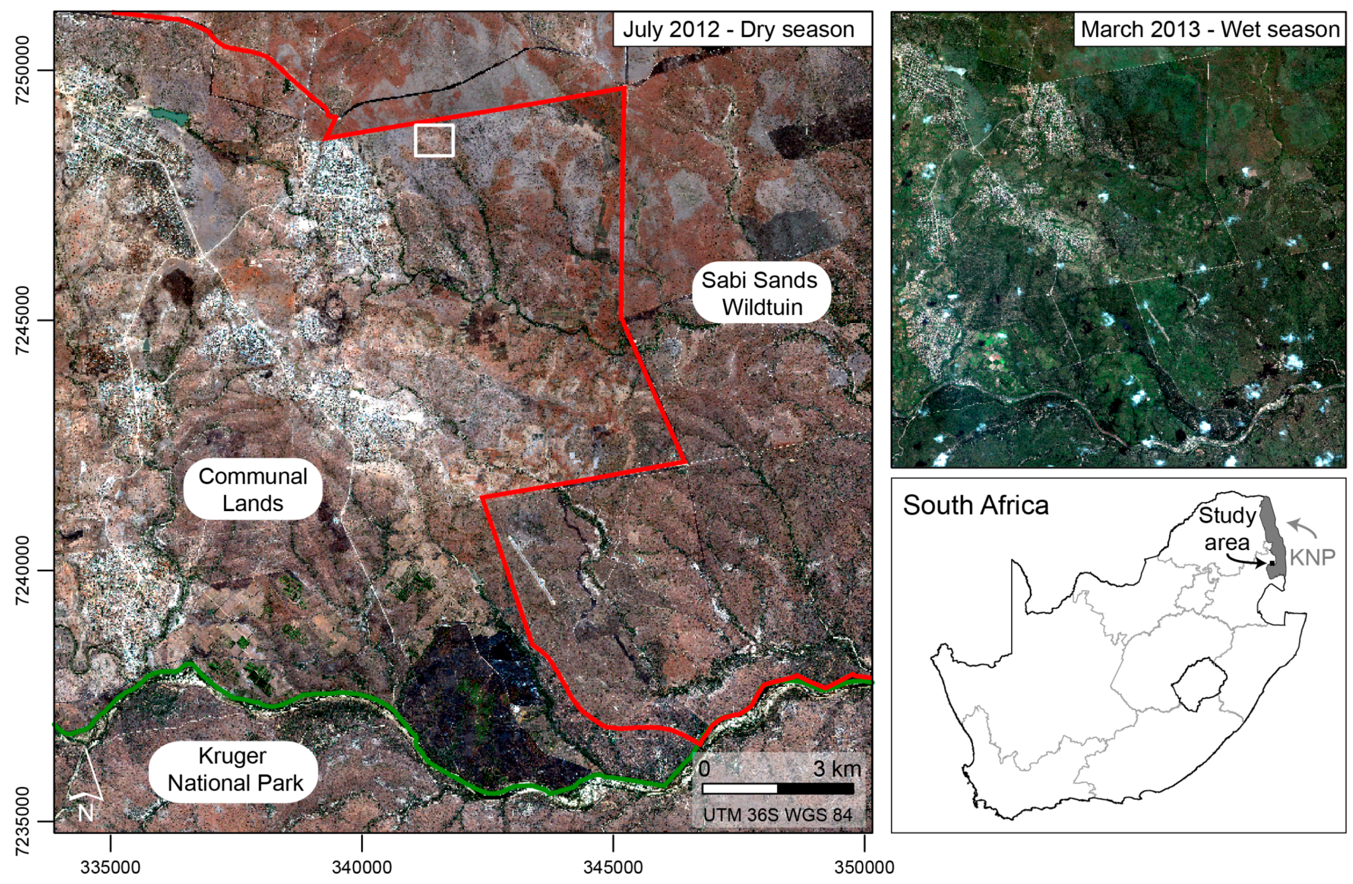
It is also important to consider seasonality while classifying savanna land cover components, due to the huge contrast in vegetation state during the wet (summer) and dry (winter) period [6]. As the environmental conditions depend on water availability, an optimal discrimination of phenological changes in different vegetation types is only possible by analyzing both wet and dry season data [7,8]. Understanding of seasonal vegetation dynamics is essential to distinguish between short-term fluctuations or long-term changes in savanna composition and productivity [9]. However, there are several challenges to overcome when discriminating land cover types from satellite imagery in tropical savanna regions. First of all, image selection is affected by dense cloud cover and a high amount of atmospheric water vapor occurring in the rainy period. These often prevent the usage of wet season scenes or create gaps in the classification maps. Despite that, wet season images are often preferred as they represent the peak of the growing season with well-developed vegetation cover and leaf-on conditions [8,10]. However, when considering fine-scale separation of savanna components, the high photosynthesis rate may confuse spectral differences between vegetation types [11]. Extended band combination of new satellite sensors recording slight differences in the vegetation reflectance can potentially contribute to solve this problem [12]. On the other hand, dry season imagery is usually cloud-free and offers better contrast between senescing herbaceous vegetation and evergreen trees [13,14]. It might however be difficult to detect leafless deciduous trees in winter scenes, as the tree canopy is significantly smaller and less defined in the leaf-off conditions. Furthermore, biochemical properties in leaves correlated with spectral information enable tree identification. That information is missing for deciduous trees in the winter period. Considering all above-mentioned issues, it is important to know how accurately savannas land cover components can be classified using winter imagery and ground truth data collected in the dry season, in comparison to commonly preferred maximum “greenness” images.
There are several remote sensing solutions useful for differentiation of land cover components in heterogeneous landscapes. Combined airborne LiDAR and hyperspectral surveys, although arguably the best suited for this application, are expensive for large scale studies, without mentioning that the availability of LiDAR or hyperspectral infrastructure in Africa is limited. Very high resolution (VHR) satellite imagery, however, affords the possibility of regional scale studies [15]. Moreover new satellite sensors, like WorldView-2 (WV-2), offer not only a very high spatial resolution but also extended and innovative spectral bands. The combination of a red-edge, yellow, and two infrared bands of WV-2 provide additional valuable information for vegetation classification [16,17,18], which may be particularly useful when spectrally similar components like shrubs and trees need to be separated. As a consequence, several studies proved the benefits of using WV-2 imagery for land cover classification of diverse landscapes (e.g., [19,20,21]).
Most land use classification studies are based on pixel-oriented approach. It is generally well accepted that pixel-based classification tends to perform better with images of relatively coarse spatial resolution [22,23]. However, fine-scale land cover classification based on VHR imagery increases the number of detectable class elements, thus the within-class spectral variance. This can make the separation of spectrally mixed land cover types more difficult [24] and leads to an increase of misclassified pixels, creating a “salt-and-pepper” effect when using a pixel-based approach [25]. An alternative classification method is the Object-Based Image Analysis (OBIA), where an image is firstly segmented into internally homogeneous segments to represent spatial objects. Segments, compared to single pixels, can be described according to a wider range of spectral and spatial features [5,26]. Furthermore, replacement of pixel values belonging to the same segment by their means lowers the variance of the complete pixels’ set (see Huygens theorem in Edwards and Cavalli-Sforza (1965) [27]). As a result, several studies have proven that object-based approaches can be very useful for mapping vegetation structure and to discriminate structural stages in vegetation [5,28,29,30]. Furthermore, different authors claimed that OBIA is better suited for classifying VHR imagery compared to pixel-based methods [23,31,32,33]. However, none of these studies tested the usability of OBIA in highly heterogeneous landscape such as African savanna for fine-scale land cover classification. Although OBIA has been proven to perform better with high resolution data, it remains unknown whether it outperforms the pixel-based approach when applied to a fine-scale mosaic of vegetation patches consisting, often, of only a few pixels.
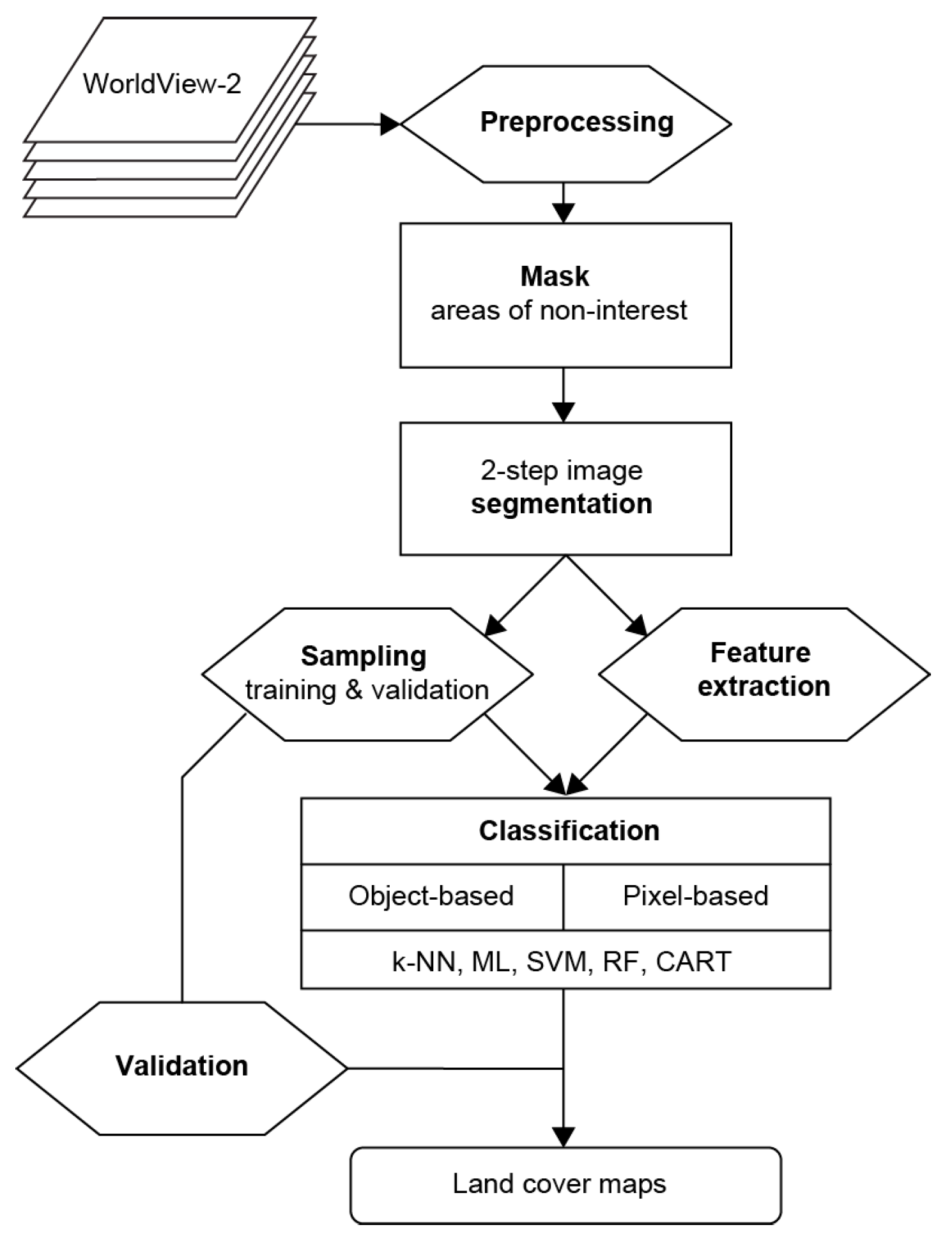
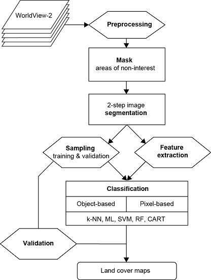
Besides the applied classification approach (pixel-based vs. OBIA), classification accuracy also largely depends on the used algorithm. Traditional methods like k-nearest neighbor (k-NN) or maximum likelihood (ML) have been used frequently in the past, but are nowadays increasingly replaced by modern and robust supervised machine learning algorithms including tree-based methods, artificial neural networks or support vector machines. Several studies compared the performance of machine learning algorithms with OBIA or pixel-based classification [31,34,35]. However, it is yet unclear which of the classifiers performs the best with OBIA and pixel-based approaches, especially when used with VHR imagery for detail separation of vegetation components in African savanna.
To our knowledge, there are no extensive studies exploring best methods for fine-scale seasonal delineation of trees, shrubs, bare soils, and grasses in African savanna. This study is the first to comprehensively investigate how best to classify land cover components of an African savanna—a biome characterized by a very high level of heterogeneity. The novelty of this study lies in the combination of several factors: the investigated biome, the fine-scale separation of land cover components, the context of seasonality, the set of tested classifiers, and the application of advanced satellite imagery. In particular we examined the performance of selected traditional and machine learning algorithms with object- and pixel-based classification approaches applied to wet and dry season WorldView-2 imagery. We hypothesized that: (1) the OBIA approach performs better than the pixel-based method in highly heterogeneous landscape of African savanna and in both seasons; (2) more advanced machine learning algorithms outperform traditional classifiers; and (3) in wet or peak productivity season, WorldView-2 scenes provide better classification results than during the leaf-off dry season.

2. Materials and Methods

2.1. Study Area

The study area covers the extent of a single WorldView-2 scene between approximately 24.85°–25.00°S and 31.35°–31.52°E in the low-lying savanna of the northeastern part of South Africa (Figure 1). The area encompasses three main land tenures: the state-owned Kruger National Park (KNP), the privately owned Sabi Sands Wildtuin/Game Reserve (SSW) and the very densely populated communal lands of Bushbuckridge (COM). The topography in the study area is gently undulating with flat patches, and with an elevation ranging between 280 and 480 m above sea level. Annual mean temperature is about 22 °C while the annual rainfall is approximately 630 mm [6]. Rains are confined to the summer (wet season) from October to May [6]. During the dry (winter) season (May to October), bush fires are frequently used for controlling shrubs and provoking nutritious green grass regrowth.
The vegetation in the study area is largely influenced by the dominant geology which consists of granite and gneiss with local intrusions of gabbro [6]. Therefore, the two dominant vegetation communities are classified as “granite lowveld” and “gabbro grassy bushveld”, [36]. The “granite lowveld” is dominated by woody communities, mainly deciduous Combretaceae with broad leaves, while grasses are sparse [36]. In contrast, “gabbro grassy bushveld” constitutes an open savanna with a dense cover of nutritious grasses and a few scattered trees and shrubs, mostly Mimosaceae (especially Acacia Spp.) with fine compound leaves and many thorns [36].

2.2. Image Acquisition and Pre-Processing

Two WorldView-2 scenes (panchromatic, 0.5 m pixel size and 8 bands multispectral, 2 m pixel size) were acquired on 15 July 2012 and 7 March 2013 (see Table 1 for acquisition parameters), which timing coincides with the dry (or winter) and wet season (or summer), respectively.
The images (including the panchromatic band) were geometrically and atmospherically corrected. As a first step, the images were orthorectified using a mathematical model based on rational polynomial coefficients (RPC) supplied by the image vendor. PCI Geomatica OrthoEngine 2013 was used for this task. An additional zero-order refinement was applied to this RPC model, using 7 accurate (post-processed to sub-meter accuracy using one-second data from the Nelspruit reference station) ground control points (GCPs), which were collected in the field using a Trimble GeoXH global positioning system (GPS). This zero-order refinement method has previously been recommended for attaining the best results with WorldView-2 imagery [37]. To remove the terrain effect, a digital elevation model (DEM) derived from a 90-m SRTM (Shuttle Radar Topography Mission) elevation data [38] was used. This was chosen because it was the best available DEM for the study area at the time. The limited spatial resolution of the DEM however led to moderate results in the geometrical correction, especially for the panchromatic images: root mean square error in 2D (RMSE 2D) of 4.4 and 1.0 pixels for the panchromatic and multispectral image, respectively.
In the next step, the images were atmospherically corrected and converted from digital numbers to reflectance values using the ATCOR2 algorithm developed by Richter [39]. Finally, the multispectral bands were resampled to 0.5 m (the resolution of the panchromatic band) using the “disaggregate” function in R software (package “raster”) [40].

2.3. Methods

The methodology used in the study is summarized in Figure 3. This workflow was run separately on both the wet and the dry season image. Firstly, a rule-based approach was implemented on each image to mask out clouds, settlements, human infrastructure, water, fields and burnt areas. Next, the images were segmented into homogenous objects for which a selection of features was calculated. Finally, a collection of training and validation samples (both object-based and pixel-based) was subsequently selected based on field data. The training samples were used to train a selection of classification algorithms, while the validation samples were used for an independent validation of the obtained land cover maps.

2.3.1. Classification of Clouds, Settlements, Human Infrastructure, Water, Fields and Large Burnt Areas

As this study focuses exclusively on natural landscapes consisting out of trees, grass, bare soil and shrubs, prior to classifying these classes, several steps were taken to mask out regions of non-interest. In particular, clouds, cloud shadows, urban settlements, water bodies, human infrastructure (roads and runways) and cultivated fields were removed, and were not taken into account for further analysis. Furthermore, a preliminary mask for large size controlled burnt plots was applied due to the ephemeral character of these areas. Clouds and clouds shadows were manually digitalized. Masking out other regions of non-interest involved a combination of thresholding and extraction based on ancillary data.

2.3.2. Image Segmentation

After masking out the areas of non-interest, image segmentation was performed using the multi-resolution bottom-up segmentation algorithm [41] embedded in eCognition 8.8 [42]. Two hierarchic segmentation levels were produced: a first (fine) level was created using only the panchromatic image as input layer, which was then grown into a second (coarse) level using 4 multispectral (Red, Red-Edge, NIR1, and NIR2) bands combined with the panchromatic image. We tested several band combinations and the final four bands have proven to provide the best visual results. Furthermore, those bands are commonly used in vegetation studies [16,17,18] and the segmented area consists mainly of different forms of vegetation. The rationale behind hierarchic segmentation approach was to first delineate small but homogenous objects (for example individual small canopies or shrubs) at the highest resolution (0.5 m) possible, and subsequently grow those objects through pair-wise merging of neighboring objects based on spectral similarity.
Required parameters (scale and compactness) for these two steps were set by using a systematic “trial-and-error” approach often employed when conducting object-based image analysis [34,43,44]. Various values for scale and compactness were tested and appropriate values, i.e., avoiding under-segmentation and over-segmentation, were thus selected based on visual inspection of the segmentation results. An overview of these values can be found in Table 2.

2.3.3. Field Data Collection and Sampling

Ground truth data for training and validation were collected during two field missions in the dry period (July 2012) and at the end of wet season (March 2013). Sampling points (876 in wet season and 713 in dry season) corresponding to the four land cover classes of interest (bare soil, tree, shrub and grass cover) and burnt areas were collected using a hand held Trimble GeoXH GPS system. To distinguish trees from shrubs, a threshold was set at a height of 2 m. Two meters was selected as this is the average minimum height of thickets of trees such as A. gerrardii and D. Cinerea [18]. Sampling point locations were mainly purposively taken based on the WorldView-2 images to cover as much of the image and vegetation-driven variance resulting from species diversity within a land cover class, environmental and management conditions, for instance geology (gabbro vs. granite) or land management (conserve vs. communal lands). The sampling was design to ensure that the data set used for land cover classifications was of good quality for all investigated classifiers and that the classification results represents the classifiers performance, rather than quality of the training data.
Based on the results of the image segmentation and the ground truth reference points, a selection of 713 (wet season image) and 876 (dry season image) coarse level homogeneous segments served as samples for the classification process. Besides the four classes of interest, two additional classes, shadow and burnt areas were incorporated in the classification. While the former was required due to the very high spatial resolution of the imagery which clearly identified tree shadows, the latter was needed because the often complex spectral signature of these burnt areas made it impossible to classify all burnt areas at once as reported in Section 3.1. In this step, burnt areas were considered as any dark area where burnt component is dominant and limits the detection of trees or shrubs, and where the grass component is suppressed. Shadows were sampled directly from the images. As a result, segments for a total of 6 classes were selected to serve as training and validation data. An overview of the number of sample segments used for each class is given in Table 3.
In order to obtain training and testing samples for the pixel-based classification that were commensurate with training and testing image objects for the different images, one single point within each of the selected image objects was randomly selected. As such, this sampling ensured that both the object-based and pixel-based classifications used training and testing/validation data gathered from the same locations.
Two thirds of the samples were selected to train the different classifiers and one third served as an independent (hold-out) validation set (Table 3). Model building and tuning of individual parameters used by the classification algorithms was accomplished through repeated k-fold cross-validation based on the training data set only (see below).

2.3.4. Feature Selection

Following the image segmentation and sampling, a set of 24 object-features likely to contribute to the object-based classification was selected (Table 4). These object-features comprised a mixture of mean band values, standard deviations and ratios, vegetation indices, texture indices and HSI transformations. This selection of features was based on a literature review and has been previously reported to substantially improve classification results (e.g., [44,45]). All object-features, except grey level co-occurrence matrix (GLCM) features such as homogeneity and entropy, were calculated in eCognition 8.8 and subsequently exported as object-feature images. Due to the size of the WorldView-2 images and the eCognition Developer processing limitations, GLCM homogeneity and entropy images [46] were calculated using the r.texture function in GRASS 7.0.
For pixel-based classification, besides band values and two vegetation indices (the normalized difference vegetation index NDVI and the Red-edge NDVI), also images of GLCM homogeneity and entropy were derived at pixel level for each of the two images (Table 4). In order to calculate these 2 texture features, an 11 × 11 window was used.

2.3.5. Classifying the Different Savanna Components

A selection of traditional, k-nearest neighbor (k-NN) and maximum likelihood (ML), and relatively modern and robust supervised machine learning algorithms like random forests (RF), classification and regression trees (CART) and support vector machine (SVM), were compared. The k-NN is a non-parametric method when the pixel/object is classified by a majority vote of its neighbors and it is assigned to a most common class among its k nearest neighbors [47]. In contrast, the ML is a parametric classifier calculating the probability that a given object or pixel belongs to a specific land cover class, and assigns it to a class to which it most likely belongs (e.g., [48]). RF, CART and SVM are non-parametric supervised machine learning algorithms. The CART model constructs rule sets by iteratively subsetting the target dataset into smaller homogeneous groups, according to defined thresholds of explanatory features. It is a single decision tree approach, which groups the target data until an end node for a defined class is reached [12]. On the contrary, RF is an ensemble of large number of decision trees, “growing” based on bootstrap samples of the original data set [49]. The predicted class is determined by majority vote from all of the decision trees [50]. Kernel based SVM likewise RF has been successfully used for classifying complex data of higher dimensionality [51]. SVM classifies pixels/objects by constructing hyperplanes in a multidimensional space that optimally (in terms of generalization error) separates cases of different class labels [52].
All 5 classifiers were used both for pixel-based and object-based classification using testing/validation data gathered from the same locations and by implementing the features listed in Table 4. The 3.1.2 version of R software for statistical computing [40] was used for the classifications. All classifiers were developed using the “caret” package within R [53], which allowed for a single consistent environment for training each of the machine learning algorithms and tuning their associated parameters. A k-fold (with here k = 5) cross-validation resampling technique was repeated 10 times on the training data set to create and optimize classification models for both pixel-based and object-based classifications using all five different classifiers. Tuning parameters were considered optimized based on classification models that achieved the highest overall classification during the cross validation process. In cross-validation, the dataset is randomly divided into k subsets of approximately equal size. A training set is then formed by combining all except one of these groups, with the omitted subset used to derive performance measures.

2.3.6. Accuracy Assessment

For each classification, a confusion matrix was calculated for the hold-out validation set, along with its overall accuracy (i.e., the percentage of correctly classified land cover types), and user and producer accuracy. The McNemar test [54,55] was used to assess the statistical significance of the following comparison: (1) pixel-based versus object-based classifications utilizing a given algorithm; and; (2) different algorithms when using either pixel-based or object-based image analysis. The McNemar test has been recommended by Footy (2004) [56] to assess whether statistically significant differences between classifications exist [56]. It has been used by several authors to statistically compare object-based and pixel-based classifications (e.g., [5,34,57,58]). The McNemar test is a parametric test, more precise and sensitive than the Kappa z-test. It is based on a chi-square (χ2) statistics, computed from two error matrices [59].

3. Results

3.1. Dry Season Classification

The dry season OBIA classifications, based on the July 2012 image (winter), achieved an overall accuracy of over 76% with the lowest score for CART, whereas the classifications based on pixels yielded an accuracy of over 68% with the minimum also for the CART algorithm (Table 5). In both classification approaches RF and SVM performed the best, reaching overall accuracies of respectively 75% and 77% when pixel-based approach was applied, and 82% and 83% with OBIA (Table 5). These two classifiers outperformed the ML, k-NN and CART algorithms, however the difference was not always significant at the 5% level (Table 6).
Considering the performance of each classifier, overall accuracies were between 6% and 8% higher for OBIA compared to their pixel-based counterpart. CART showed the biggest improvement in overall accuracy with 8% (Table 5). This increase in accuracy was significant at the 5% level for all classifiers (Table 7).
Within individual land cover classes and considering the OBIA approach, very good producer accuracies for the best classifier were obtained for bare soil, shadow, tree and burnt areas (>90%) (Table 5). However, the producer accuracy of the latter class was even higher with pixel-based approach (100% for RF and SVM). The lowest producer and user accuracy for the best algorithm within the class was found for shrubs (64% for ML and 76% for SVM). This class had also the lowest producer and user accuracy when considering pixel-based classification (56% for SVM and 67% for k-NN). Very high user accuracies (≥90%) for the best classifier and with OBIA were found for bare soil, burnt areas and shadow.
A map of land cover classes for the dry period using the best classifier and classification approach (SVM, OBIA) is presented in Figure 4. A visual inspection of this map revealed an overall high level of consistency with the WorldView-2 image (Figure 2). However, based on ground truth data we found that in some areas shrubs were confused with grass or trees.

3.2. Wet Season Classification

For the March 2013 OBIA classification, the considered algorithms achieved an overall accuracy of over 85% with the minimum score obtained for k-NN. The pixel-based algorithms showed much lower values with a minimum score of 73% for CART (Table 8). Generally, RF and SVM were again found to be the best classifiers producing very similar results in terms of overall accuracy: 93% and 92% for OBIA, respectively, and 83% for pixel-based (Table 8). They clearly outperformed the ML, k-NN and CART classifiers although the difference was not always significant at the 5% level (Table 6).
For most classifiers, overall accuracies where on average about 10% lower for the pixel-based approach than the object-based approach. These differences were found to be always significant at the 5% level (Table 7). The biggest improvement in accuracy (15%) was found for the CART algorithm and the smallest (8%) for ML (Table 8).
Comparing individual land cover classes for the OBIA approach, all classes had producer and user accuracies for the best classifier (RF) higher than 90% (Table 8). The highest, 100% producer and user accuracy was found for the bare soil, burnt, shadow classes. The tree class showed a very high producer accuracy of 99% for ML. Considering all algorithms, very few accuracy metrics were found below 80%. Generally, the lowest producer accuracy was found for shrubs and grass (below 93%). The latter class had also the lowest user accuracy (below 92%). When considering the pixel-based approach, user and producer accuracies for individual classes were found to be lower than the OBIA results, with exception of bare soil and shadow, which had accuracies of 100%.
Based on these results the best classifier and classification method (RF, OBIA) was used to create the final land cover map illustrated in Figure 4. The visual inspection of this map showed very high level of consistency with the WorldView-2 image color composites and the ground truth data (Figure 2).

3.3. Seasonal Comparison

Comparing the classification results from both seasons, the image of March 2013 representing the wet period had much higher overall accuracies for both classification approaches and every classifier. However, the seasonal difference in classifier performance was stronger for OBIA. The overall accuracy of the best classifiers for the wet season classification (RF, SMV) was 11% and 9% higher than for the dry season when using OBIA, and 8% and 6% higher when pixel-based classification was applied, respectively (Table 5 and Table 8). K-NN was the algorithm that produced the lowest difference between the two dates, for both OBIA and pixel-based approaches.
Most individual land cover classes had higher user and producer accuracy in the wet season classification compared to the dry season. However, there were also differences according to the classification approach. Pixel-based methods exhibited lower user and producer accuracies during the wet season for about 37% of the cases irrespective of the algorithm used. Poorer performances for the wet season with pixel-based approach were observed mostly for the burnt class (up to 35% decrease of producer accuracy), and for the class tree (up to 13% decrease of producer accuracy).
When comparing the user accuracy and the best performers (OBIA, RF and SMV) the wet season outperformed the dry season on all counts apart for the bare soil and burn area mapped with SVM (−1% and −4%, respectively). The largest improvement was observed for the shrub class (+21% for SVM and +29% for RF), with moderate improvement for the grass and tree class (6%–11%).

3.4. Feature Importance

The relevance of the WorldView-2 features for the delineation of land cover components of the African savanna using random forest classifier with pixel-based or OBIA approach is illustrated in Figure 5. The variables importance was calculated as a scaled version (from 0 to 100) of the mean decrease in Gini Index. Feature importance analyses showed variations between classification approaches and between seasons. However, in both approaches and for both seasons panchromatic band appeared to be the most important variable. Green, yellow, red, red-edge, NIR1 and NIR2 bands as well as NDVI and red-edge NDVI were found to be more important when random forest was applied to the wet season imagery.

4. Discussion

Findings of this study revealed that the classification based on WV-2 imagery produces high accuracy results regardless of the used classification approach. The combination of very high spatial resolution and extended spectral bands (especially yellow and red-edge) of WorldView-2 constitute an invaluable and unique dataset to discriminate woody, herbaceous, and bare components of African savannas. Advantages of using WV-2 images for fine-scale land cover classification of urban and natural landscapes were also reported by other authors (e.g., [7,48,49]). However, this is the first time that WV-2 was used for fine-scale classification of African savannas, proving effectiveness of this imagery in highly heterogeneous landscape. With WV-2 images we were able to classify individual trees, tree clumps, shrub patches, grass and bare soil, moving one step further from the “traditional” savanna land cover mapping with mixed components into more discrete classification. This might not be possible when applying IKONOS or Landsat imagery [17,60]. WV-2 provides the degree of spatial detail and geometric precision comparable to aerial photographs [61] and multispectral information facilitating more options for digital analysis [
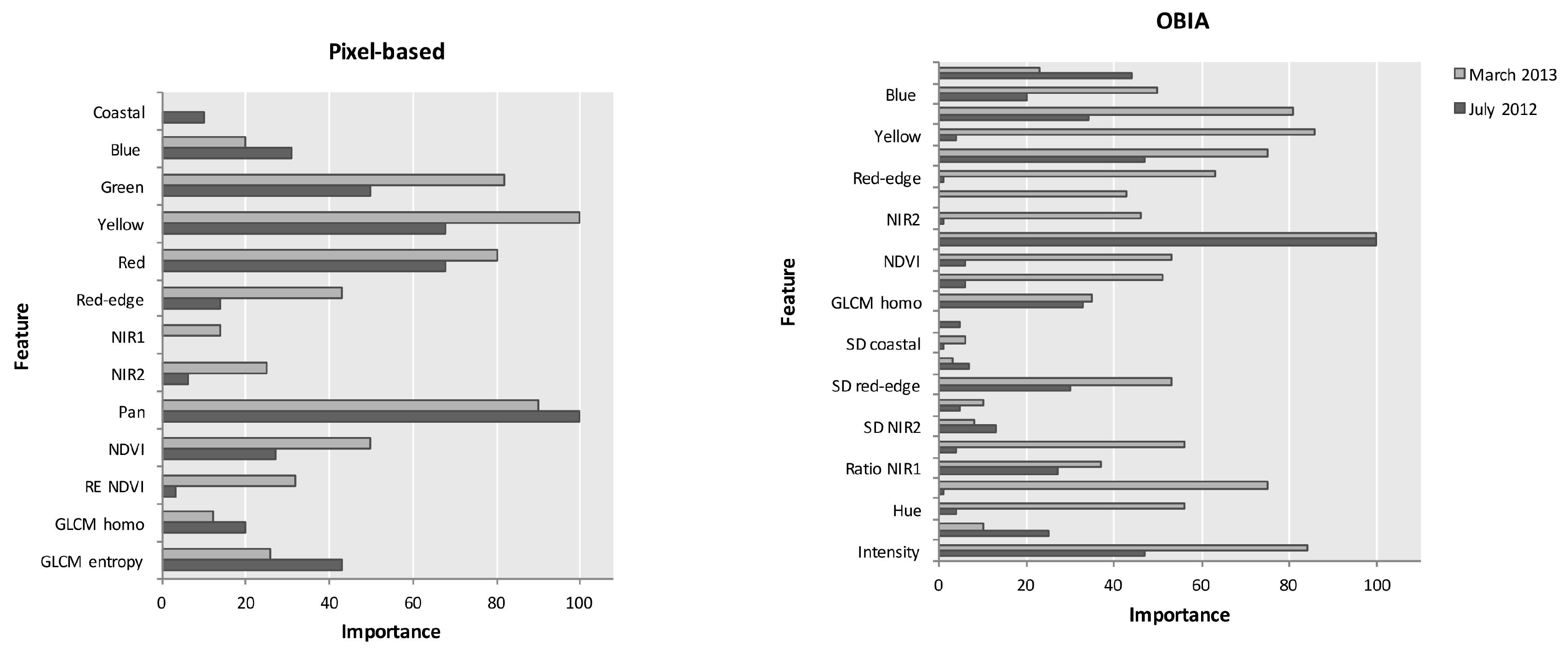
7]. The high accuracies achieved in this study can be explained by the fact that WorldView-2 provides not only a high spatial resolution but also a unique band combination. Based on random forest feature importance, we found that yellow and red-edge band in pick productivity season are important in discrimination of vegetation components in savanna ecosystem. The contribution of these bands in mapping vegetation components was reported by several authors [7,62,63]. Yellow and red-edge band are able to record variations in pigment concentration/content (e.g., chlorophyll, carotenoids, anthocyanin) in plants enabling detection of species or vegetation communities [7,17]. Only LiDAR and/or airborne hyperspectral imagery can produce similar or better classification results than WorldView-2. However, as these techniques are costly, require substantial preprocessing and are often not suitable for regional scale mapping, the methodology used in this study provides a valuable alternative.
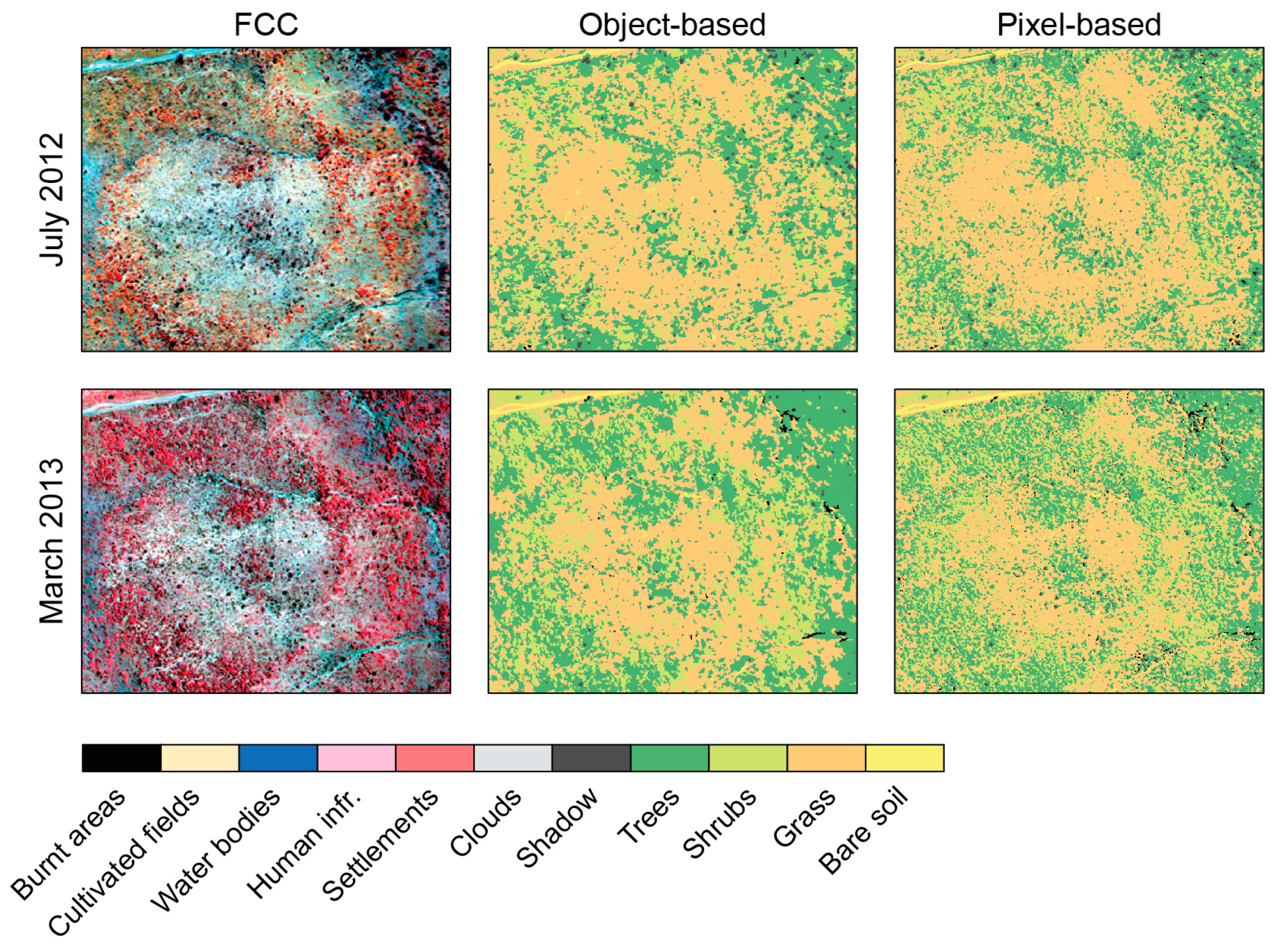
In our study, both pixel- and object-based classifications generally produced high quality results or accuracies (≥77%) regardless of the considered season. However the latter approach had a significantly higher accuracy for almost every classifier with the highest overall accuracy score of 93%. This is consistent with several other studies indicating superiority of using OBIA in a range of environments [5,31,64]. In particular, Whiteside et al. (2011) [5] concluded that OBIA outperforms pixel-based classification for medium and high resolution satellite imagery in Australian savannas. Moreover, study of Gibbes et al. (2010) [64] indicates that OBIA has a great potential in discriminating African woodland savanna from shrubby dominated and grassland patches using IKONOS high resolution imagery. Our study goes further, demonstrating that object-based classification of imagery characterized by a small pixel size and 8 spectral bands provides tools for fine level differentiation of spectrally similar vegetation components in the African savanna ecosystem. In the classification approach based on objects, thanks to hierarchic segmentation, very small objects of similar spectral information, like tree crowns, shrubs and shrub/tree patches, can be delineated, which is not possible with pixel-based methods. It leads to more thematically consistent mapping, eliminating the “salt-and-pepper” effect appearing on maps generated using pixel-based method. This is evidenced when comparing our results of OBIA and pixel-based approach for the best performing classifiers: trees and shrubs were found to have one of the highest improvements in the user accuracy in both seasons. A better performance of OBIA over pixel-based method with WorldView-2 imagery in detection of woody vegetation or even tree species was also reported by Ghosh and Joshi (2014) [7] and Immitzer et al. (2012) [62]. Furthermore, our results suggest that OBIA can be useful in crown shadow detection in the dry season, when the spectral information from the shadowed area is more consistent as it is not confused by a still strong photosynthesis signal of underlying vegetation.
All tested classifiers (except of ML in dry season classification) performed significantly better with OBIA. This is consistent with the study of Ghosh and Joshi (2014) [7] when SVM and RF classifiers produced much higher accuracy of fine-scale bamboo mapping with OBIA compared to pixel-based methods. However, Duro et al. (2012) [34] did not find any statistically significant differences in performance of CART, SVM and RF between the two classification methods using medium resolution imagery. These results might indicate that the difference in classifier performance between OBIA and pixel-based methods is more pronounced with increasing spatial resolution. Overall, SVM and RF outperformed other classifiers in both approaches and regardless the season. SVM and RF algorithms have been previously successfully applied in vegetation mapping with high and very high resolution imagery [34,62,65]. Both classifiers are non-parametric, thus do not assume a known statistical distribution of the data. This allows SVM and RF to outperform widely used classification methods based on maximum likelihood, as the remotely sensed data usually have unknown distributions [52,66]. Furthermore, one of the most important and useful in land cover classification characteristics of SVM and RF is their ability to well generalize from a limited amount of training data [52,62]. Pal (2005) [67] and Duro et al. (2012) [34] reported that both SVM and RF can produce similar classification accuracies which supports our findings. However, to achieve the best classification results with SVM the number of input features and amount of training data should be well balanced, as the accuracy of a classification by SVM has proven to decline with more features especially when using small training sample [7,68]. On the contrary, RF in comparison to SVM handles much better the variable collinearity, therefore can produce high accuracy results with more variables included in the model.
All surfaces show some degree of spectral reflectance anisotropy when illuminated by sunlight, which is described by the Bidirectional Reflectance Distribution Function (BRDF) [69]. Therefore it is important to note, that given the varying viewing angles the BRDF might have an effect on the classification accuracy results presented in this study, as for instance showed by Sue et al. (2009) [69], Vanonckelen et al. (2013) [70] and Wu and Cihlar (1995) [71].
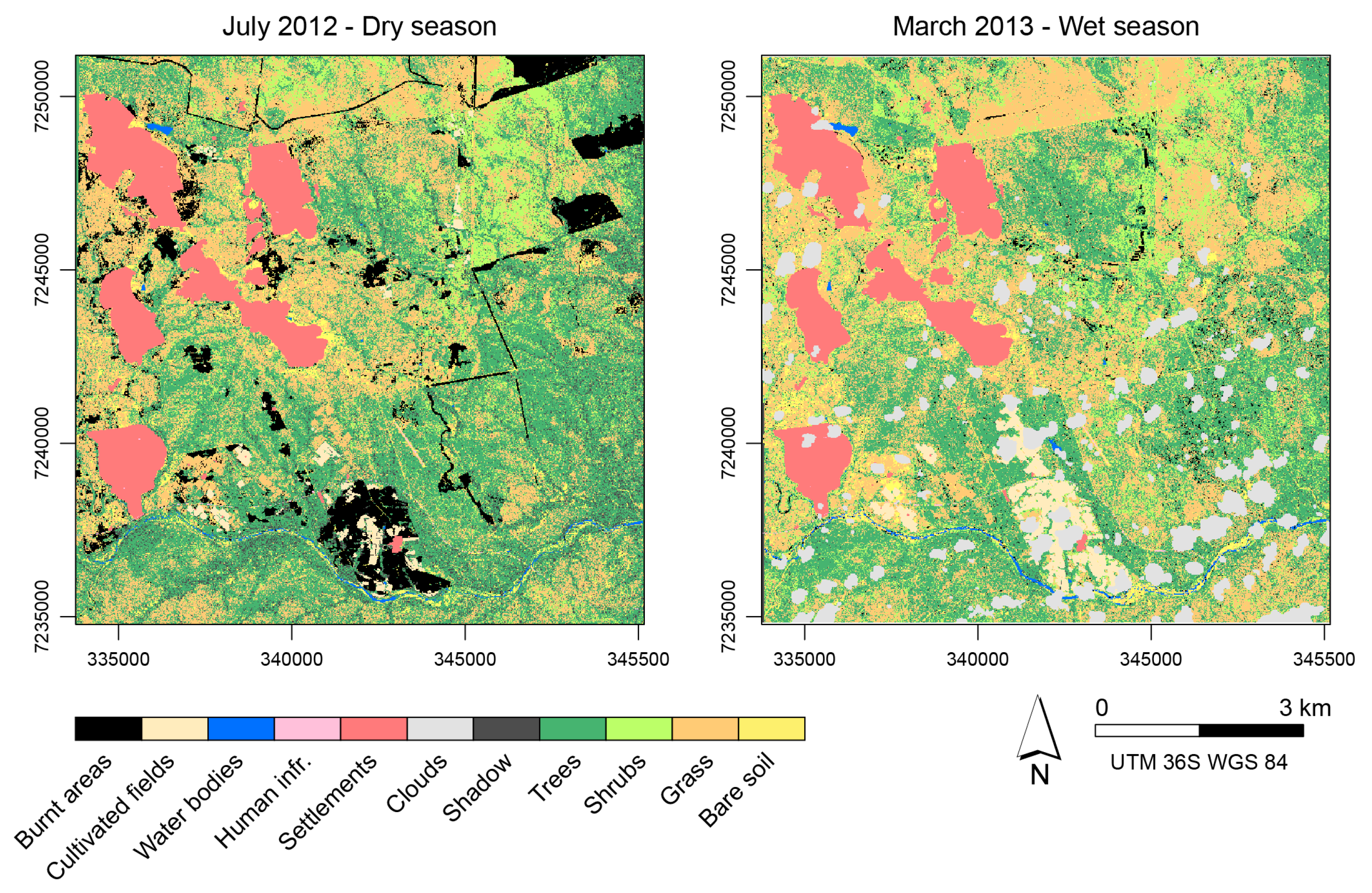
Our study demonstrates that it is possible to successfully distinguish savanna land cover components during peak vegetation productivity (March, end of summer) using VHR WV-2 imagery. Although the results of dry season classifications were also satisfactory, their accuracies were on average 10% lower than during the wet season. The latter result is however particularly useful as often, wet season imagery, although providing the best classification accuracy, is not available due to the persistent cloud cover. Wet season imagery provided much better results in discriminating shrubs compared to the dry season. Shrubs are generally difficult to separate due to their smaller, in comparison with trees, canopy sizes and poorly defined canopy shapes (e.g., multiple stems and coppices). They are therefore often confused with either smaller trees or higher herbaceous vegetation. As shrub cover is well developed during the rainy season, its enriched spectral information makes it then easier to differentiate with 8-band VHR imagery like WV-2. Besides shrubs, also bare soil showed higher accuracies for the wet season imagery. This can be attributed to the fact that in the dry season bare soil might be confused with wilting grasses or burnt lands. Interestingly, the WV-2 imagery combined with OBIA was very successful (producer accuracy of 91%) in detecting tree cover in the dry season when deciduous trees are mostly leafless. This is probably due to the small pixel size allowing accurate delineation of the leafless tree branches during segmentation process, combined with a set of texture features improving the classification results. Furthermore, as the deciduous tree species are not the major contributors to canopy characteristics in the study area, the remaining evergreen species in dry season contrast stronger in reflectance with the senescing grasses, becoming easier to classify. Similar results were found by Boggs (2010) [14], who reported that a combination of QuickBird imagery and OBIA produces high accuracy results of dry season tree cover detection in Kruger National Park.
A future possible improvement to the fine-scale classification of savanna biome is to apply multi-temporal WV-2 images with OBIA. The multi-temporal approach in vegetation classification was successfully used by several authors proving superiority over single image/season classification [9,72]. Covering different phenological stages of vegetation could improve recognition of grass, shrubs and trees in savanna. However, application of fine-scale multi-temporal images requires a very high resolution digital surface models. The necessity of proper images alignment might constitute a limiting factor for application of multi-temporal approach.

5. Conclusions

This study has investigated the potential of WorldView-2 imagery with very high spatial and spectral resolution in fine-scale seasonal mapping of African savanna land cover components. The performances of object- and pixel-based classification approaches were compared testing both traditional and more advanced, machine learning classifiers. Generally, classification of WV-2 imagery produced high mapping accuracies regardless the considered season or classification method. However, the best results were achieved for the wet season using OBIA and SVM or RF algorithms. The study has shown that the combination of OBIA with VHR WV-2 imagery is very successful in tree cover detection, even during the leaf-off period. Findings of this study demonstrate that WV-2 imagery with OBIA and advanced machine learning classifiers, like SVM and RF, constitute a very good alternative for regional fine-scale land cover classification of African savanna.

Acknowledgments

This study was possible through the grant provided by the Belgian Science Policy Office (BELSPO). Logistical and field support was provided by South African National Parks and Sabi Sands Wildtuin, especially by Sandra MacFadyen, Rheinhardt Scholtz and Michael Grover.

Author Contributions

Żaneta Kaszta conceived the study and wrote the paper with discussions and contributions from all co-authors. Ruben Van De Kerchove analyzed the data. Eléonore Wolff and Reneud Matthieu coordinated the work, and helped in designing the research concept and workflow. Abel Ramoelo, Sabelo Mandosela and Moses Azong Cho helped to outline and edit the manuscript structure.

Conflicts of Interest

The authors declare no conflict of interest.

References

  1. Chapin, F.S.; Matson, P.A.; Vitousek, P. Principles of Terrestrial Ecosystem Ecology; Springer-Verlag: New York, NY, USA, 2002. [Google Scholar]
  2. Williams, C.A.; Hanan, N.P.; Neff, J.C.; Scholes, R.J.; Berry, J.A.; Denning, A.S.; Baker, D.F. Africa and the global carbon cycle. Carbon Balanc. Manag. 2007, 7, 2–3. [Google Scholar] [CrossRef] [PubMed]
  3. Gessner, U.; Machwitz, M.; Conrad, C.; Dech, S. Estimating the fractional cover of growth forms and bare surface in savannas. A multi-resolution approach based on regression tree ensembles. Remote Sens. Environ. 2013, 129, 90–102. [Google Scholar] [CrossRef] [Green Version]
  4. Latifovic, R.; Olthof, I. Accuracy assessment using sub-pixel fractional error matrices of global land cover products derived from satellite data. Remote Sens. Environ. 2004, 90, 153–165. [Google Scholar] [CrossRef]
  5. Whiteside, T.G.; Boggs, G.S.; Maier, S.W. Comparing object-based and pixel-based classifications for mapping savannas. Int. J. Appl. Earth Obs. Geoinf. 2011, 13, 884–893. [Google Scholar] [CrossRef]
  6. Venter, F.J.; Scholes, R.J.; Eckhardt, H.C. The abiotic template and its associated vegetation pattern. In The Kruger Experience: Ecology and Management of Savanna Heterogeneity; Du Toit, J., Biggs, H., Rogers, K.H., Eds.; Island Press: London, UK, 2003; pp. 83–129. [Google Scholar]
  7. Ghosh, A.; Joshi, P.K. A comparison of selected classification algorithms for mapping bamboo patches in lower Gangetic plains using very high resolution WorldView 2 imagery. Int. J. Appl. Earth Obs. Geoinf. 2014, 26, 298–311. [Google Scholar] [CrossRef]
  8. Liu, J.; Heiskanen, J.; Aynekulu, E.; Pellikka, P.K.E. Seasonal variation of land cover classification accuracy of Landsat 8 images in Burkina Faso. Int. Arch. Photogramm. Remote Sens. Spat. Inf. Sci. 2015, 40, 455–460. [Google Scholar] [CrossRef]
  9. Hassler, S.K.; Kreyling, J.; Beierkuhnlein, C.; Eisold, J.; Samimi, C.; Wagenseil, H.; Jentsch, A. Vegetation pattern divergence between dry and wet season in a semiarid savanna—Spatio-temporal dynamics of plant diversity in Northwest Namibia. J. Arid Environ. 2010, 74, 1516–1524. [Google Scholar] [CrossRef]
  10. Zhu, X.; Liu, D. Accurate mapping of forest types using dense seasonal Landsat time-series. ISPRS J. Photogramm. Remote Sens. 2014, 96, 1–11. [Google Scholar] [CrossRef]
  11. Sawada, H.; Araki, M.; Chappell, N.A.; LaFrankie, J.V.; Shimizu, A. Forest Environments in the Mekong River Basin; Springer: Tokyo, Japan, 2007. [Google Scholar]
  12. Naidoo, L.; Cho, M.A.; Mathieu, R.; Asner, G. Classification of savanna tree species, in the Greater Kruger National Park region, by integrating hyperspectral and LiDAR data in a Random Forest data mining environment. ISPRS J. Photogramm. Remote Sens. 2012, 69, 167–179. [Google Scholar] [CrossRef]
  13. Lucas, R.M.; Held, A.; Phinn, S.R.; Saatchi, S. Tropical forests. In Remote Sensing for Natural Resource Management and Environmental Monitoring; John Wiley & Sons, Inc.: Hoboken, NJ, USA, 2004; pp. 239–316. [Google Scholar]
  14. Boggs, G.S. Assessment of SPOT 5 and QuickBird remotely sensed imagery for mapping tree cover in savannas. Int. J. Appl. Earth Obs. Geoinf. 2010, 12, 217–224. [Google Scholar] [CrossRef]
  15. Goetz, S.J.; Wright, R.K.; Smith, A.J.; Zinecker, E.; Schaub, E. IKONOS imagery for resource management: Tree cover, impervious surfaces, and riparian buffer analyses in the mid-Atlantic region. Remote Sens. Environ. 2003, 88, 195–208. [Google Scholar] [CrossRef]
  16. Dlamini, W.M. Multispectral detection of invasive alien plants from very high resolution 8-band satellite imagery using probabilistic graphical models. Digit. Globe 2010, 8, 1–17. [Google Scholar]
  17. Pu, R.; Landry, S. A comparative analysis of high spatial resolution IKONOS and WorldView-2 imagery for mapping urban tree species. Remote Sens. Environ. 2012, 124, 516–533. [Google Scholar] [CrossRef]
  18. Cho, M.A.; Mathieu, R.; Asner, G.P.; Naidoo, L.; van Aardt, J.; Ramoelo, A.; Debba, P.; Wessels, K.; Main, R.; Smit, I.P.J.; Erasmus, B. Mapping tree species composition in South African savannas using an integrated airborne spectral and LiDAR system. Remote Sens. Environ. 2012, 125, 214–226. [Google Scholar] [CrossRef]
  19. Novack, T.; Esch, T.; Kux, H.; Stilla, U. Machine learning comparison between WorldView-2 and QuickBird-2-simulated imagery regarding object-based urban land cover classification. Remote Sens. 2011, 3, 2263–2282. [Google Scholar] [CrossRef]
  20. Elsharkawy, A.; Elhabiby, M.; El-sheimy, N. Improvement in the detection of land cover classes using the Worldview-2 imagery. In Proceedings of the ASPRS 2012 Annual Conference, Sacramento, CA, USA, 19–23 Much 2012; pp. 19–23.
  21. Belgiu, M.; Drǎguţ, L.; Strobl, J. Quantitative evaluation of variations in rule-based classifications of land cover in urban neighbourhoods using WorldView-2 imagery. ISPRS J. Photogramm. Remote Sens. 2014, 87, 205–215. [Google Scholar] [CrossRef] [PubMed]
  22. Niemeyer, I.; Canty, M.J. Pixel-based and object-oriented change detection analysis using high-resolution imagery. In Proceedings of the 25th Symposium on Safeguards and Nuclear Material Management, Stockholm, Sweden, 13–15 May 2003; pp. 2133–2136.
  23. Oruc, M.; Marangoz, A.M.; Buyuksalih, G. Comparison of pixel-based and object-oriented classification approaches using Landsat-7 ETM spectral bands. In Proceedings of the IRSPS 2004 Annual Conference, Istanbul, Turkey, 12–23 July 2004; pp. 19–23.
  24. Shaban, M.A.; Dikshit, O. Improvement of classification in urban areas by the use of textural features: The case study of Lucknow city, Uttar Pradesh. Int. J. Remote Sens. 2001, 22, 565–593. [Google Scholar] [CrossRef]
  25. Blaschke, T.; Lang, S.; Lorup, E.; Strobl, J.; Zeil, P. Object-oriented image processing in an integrated GIS/remote sensing environment and perspectives for environmental applications. Environ. Inf. Plan. Polit. Public 2000, 2, 555–570. [Google Scholar]
  26. Blaschke, T. Object based image analysis for remote sensing. ISPRS J. Photogramm. Remote Sens. 2010, 65, 2–16. [Google Scholar] [CrossRef]
  27. Edwards, A.W.F.; Cavalli-Sforza, L.L. A method for cluster analysis. Biometrics 1965, 21, 362–375. [Google Scholar] [CrossRef] [PubMed]
  28. Johansen, K.; Coops, N.C.; Gergel, S.E.; Stange, Y. Application of high spatial resolution satellite imagery for riparian and forest ecosystem classification. Remote Sens. Environ. 2007, 110, 29–44. [Google Scholar] [CrossRef]
  29. Mallinis, G.; Koutsias, N.; Tsakiri-Strati, M.; Karteris, M. Object-based classification using Quickbird imagery for delineating forest vegetation polygons in a Mediterranean test site. ISPRS J. Photogramm. Remote Sens. 2008, 63, 237–250. [Google Scholar] [CrossRef]
  30. Stow, D.; Hamada, Y.; Coulter, L.; Anguelova, Z. Monitoring shrubland habitat changes through object-based change identification with airborne multispectral imagery. Remote Sens. Environ. 2008, 112, 1051–1061. [Google Scholar] [CrossRef]
  31. Castillejo-González, I.L.; López-Granados, F.; García-Ferrer, A.; Peña-Barragán, J.M.; Jurado-Expósito, M.; de la Orden, M.S.; González-Audicana, M. Object- and pixel-based analysis for mapping crops and their agro-environmental associated measures using QuickBird imagery. Comput. Electron. Agric. 2009, 68, 207–215. [Google Scholar] [CrossRef]
  32. Mansor, S.; Hong, W.T.; Shariff, A.R.M. Object oriented classification for land cover mapping. In Proceedings of the Map Asia, Bangkok, Tailand, 7–9 August 2002.
  33. Willhauck, G.; Schneider, T.; de Kok, R.; Ammer, U. Comparison of object oriented classification techniques and standard image analysis for the use of change detection between SPOT multispectral satellite images and aerial photos. In Proceedings of XIX ISPRS Congress, Amsterdam, The Netherlands, 16–23 July 2000; Volume 33, pp. 35–42.
  34. Duro, D.C.; Franklin, S.E.; Dubé, M.G. A comparison of pixel-based and object-based image analysis with selected machine learning algorithms for the classification of agricultural landscapes using SPOT-5 HRG imagery. Remote Sens. Environ. 2012, 118, 259–272. [Google Scholar] [CrossRef]
  35. Du, P.; Xia, J.; Zhang, W.; Tan, K.; Liu, Y.; Liu, S. Multiple classifier system for remote sensing image classification: A review. Sensors 2012, 12, 4764–4792. [Google Scholar] [CrossRef] [PubMed]
  36. Mucina, L.; Rutherford, M.C. The Vegetation of South Africa, Lesotho and Swaziland; South African National Biodiversity Institute: Pretoria, South Africa, 2006. [Google Scholar]
  37. Aguilar, M.A.; Saldaña, M.D.M.; Aguilar, F.J. Assessing geometric accuracy of the orthorectification process from GeoEye-1 and WorldView-2 panchromatic images. Int. J. Appl. Earth Obs. Geoinf. 2012, 21, 427–435. [Google Scholar] [CrossRef]
  38. Jarvis, A.; Reuter, H.I.; Nelson, A.; Guevara, E. Hole-Filled SRTM for The Globe Version 4. Available online: http://srtm.csi.cgiar.org (accessed on 20 June 2012).
  39. Richter, R.; Schläpfer, D. Atmospheric/Topographic Correction for Satellite Imagery. ATCOR-2/3 User Guide, Version 8.3; ReSe Applications Schläpfer: Wil, Switzerland, 2013. [Google Scholar]
  40. R Development Core Team. R: A Language and Environment for Statistical Computing; R Foundation for Statistical Computing Team: Vienna, Austria, 2012. [Google Scholar]
  41. Baatz, M.; Schäpe, A. Multiresolution segmentation: An optimization approach for high quality multi-scale image segmentation. In Angewandte Geographische Informationsverarbeitung XII; Strobl, J., Blaschke, T., Griesebner, G., Eds.; Wichann-Verlag: Heidelberg, Germany, 2000; pp. 12–23. [Google Scholar]
  42. Trimble eCognition® Developer 8.8 Reference Book. Available online: http://www.ecognition.com/ (accessed on 5 January 2012).
  43. Mathieu, R.; Aryal, J.; Chong, A.K. Object-based classification of IKONOS imagery for mapping large-scale vegetation communities in urban areas. Sensors 2007, 7, 2860–2880. [Google Scholar] [CrossRef]
  44. Myint, S.W.; Gober, P.; Brazel, A.; Grossman-Clarke, S.; Weng, Q. Per-pixel vs. object-based classification of urban land cover extraction using high spatial resolution imagery. Remote Sens. Environ. 2011, 115, 1145–1161. [Google Scholar] [CrossRef]
  45. Stumpf, A.; Kerle, N. Object-oriented mapping of landslides using Random Forests. Remote Sens. Environ. 2011, 115, 2564–2577. [Google Scholar] [CrossRef]
  46. Haralick, R.M.; Shanmugam, K.; Dinstein, I. Textural features for image classification. IEEE Trans. Syst. Man Cybern. 1973, SMC-3, 610–621. [Google Scholar] [CrossRef]
  47. Cover, T.; Hart, P. Nearest neighbor pattern classification. IEEE Trans. Inf. Theory 1967, 13, 21–27. [Google Scholar] [CrossRef]
  48. Foody, G.M.; Campbell, N.A.; Trodd, N.M.; Wood, T.F. Derivation and applications of probabilistic measures of class membership from the maximum-likelihood classification. Photogramm. Eng. Remote Sens. 1992, 58, 1335–1341. [Google Scholar]
  49. Breiman, L. Random forests. Mach. Learn. 2001, 45, 5–32. [Google Scholar] [CrossRef]
  50. Cutler, D.R.; Edwards, T.C.; Beard, K.H.; Cutler, A.; Hess, K.T.; Gibson, J.; Lawler, J.J. Random forests for classification in ecology. Ecology 2007, 88, 2783–2792. [Google Scholar] [CrossRef] [PubMed]
  51. Dalponte, M.; Bruzzone, L.; Gianelle, D. Tree species classification in the southern Alps based on the fusion of very high geometrical resolution multispectral/hyperspectral images and LiDAR data. Remote Sens. Environ. 2012, 123, 258–270. [Google Scholar] [CrossRef]
  52. Mountrakis, G.; Im, J.; Ogole, C. Support vector machines in remote sensing: A review. ISPRS J. Photogramm. Remote Sens. 2011, 66, 247–259. [Google Scholar] [CrossRef]
  53. Kuhn, M. Building Predictive Models in R Using the caret Package. J. Stat. Softw. 2010, 28. [Google Scholar]
  54. Agresti, A. Categorical Data Analysis; John Wiley & Sons, Inc: Hoboken, NJ, USA, 2002. [Google Scholar]
  55. Zar, J.H. Biostatistical Analysis, 5th ed.; Prentice Hall: Upper Saddle River, NJ, USA, 2009. [Google Scholar]
  56. Foody, G.M. Thematic map comparison: Evaluating the statistical significance of differences in classification accuracy. Photogramm. Eng. Remote Sens. 2004, 70, 627–633. [Google Scholar] [CrossRef]
  57. Dingle Robertson, L.; King, D.J. Comparison of pixel-and object-based classification in land cover change mapping. Int. J. Remote Sens. 2011, 32, 1505–1529. [Google Scholar] [CrossRef]
  58. Gao, Y.; Mas, J.-F.; Maathuis, B.H.P.; Zhang, X.; van Dijk, P.M. Comparison of pixel-based and object-oriented image classification approaches—A case study in a coal fire area, Wuda, Inner Mongolia, China. Int. J. Remote Sens. 2006, 27, 4039–4055. [Google Scholar]
  59. Manandhar, R.; Odeh, I.O.A.; Ancev, T. Improving the accuracy of land use and land cover classification of Landsat data using post-classification enhancement. Remote Sens. 2009, 1, 330–344. [Google Scholar] [CrossRef]
  60. Stuart, N.; Barratt, T.; Place, C. Classifying the neotropical savannas of Belize using remote sensing and ground survey. J. Biogeogr. 2006, 33, 476–490. [Google Scholar] [CrossRef]
  61. Turner, W.; Spector, S.; Gardiner, N.; Fladeland, M.; Sterling, E.; Steininger, M. Remote sensing for biodiversity science and conservation. Trends Ecol. Evol. 2003, 18, 306–314. [Google Scholar] [CrossRef]
  62. Immitzer, M.; Atzberger, C.; Koukal, T. Tree species classification with Random Forest using very high spatial resolution 8-band WorldView-2 satellite data. Remote Sens. 2012, 4, 2661–2693. [Google Scholar] [CrossRef]
  63. Pu, R. Broadleaf species recognition with in situ hyperspectral data. Int. J. Remote Sens. 2009, 30, 2759–2779. [Google Scholar] [CrossRef]
  64. Gibbes, C.; Adhikari, S.; Rostant, L.; Southworth, J.; Qiu, Y. Application of object based classification and high resolution satellite imagery for savanna ecosystem analysis. Remote Sens. 2010, 2, 2748–2772. [Google Scholar] [CrossRef]
  65. Löw, F.; Conrad, C.; Michel, U. Decision fusion and non-parametric classifiers for land use mapping using multi-temporal RapidEye data. ISPRS J. Photogramm. Remote Sens. 2015, 108, 191–204. [Google Scholar] [CrossRef]
  66. Rodriguez-Galiano, V.F.; Ghimire, B.; Rogan, J.; Chica-Olmo, M.; Rigol-Sanchez, J.P. An assessment of the effectiveness of a random forest classifier for land-cover classification. ISPRS J. Photogramm. Remote Sens. 2012, 67, 93–104. [Google Scholar] [CrossRef]
  67. Pal, M. Random forest classifier for remote sensing classification. Int. J. Remote Sens. 2005, 26, 217–222. [Google Scholar] [CrossRef]
  68. Pal, M.; Foody, G.M. Feature selection for classification of hyperspectral data by SVM. IEEE Trans. Geosci. Remote Sens. 2010, 48, 2297–2307. [Google Scholar] [CrossRef]
  69. Su, L.; Huang, Y.; Chopping, M.J.; Rango, A.; Martonchik, J.V. An empirical study on the utility of BRDF model parameters and topographic parameters for mapping vegetation in a semi-arid region with MISR imagery. Int. J. Remote Sens. 2009, 30, 3463–3483. [Google Scholar] [CrossRef]
  70. Vanonckelen, S.; Lhermitte, S.; van Rompaey, A. The effect of atmospheric and topographic correction methods on land cover classification accuracy. Int. J. Appl. Earth Obs. Geoinf. 2013, 24, 9–21. [Google Scholar] [CrossRef]
  71. Wu, A.; Li, Z.; Cihlar, J. Effect of land cover type and greenness on advanced very high resolution radiometer bidirectional reflectances: Analysis and removal. J. Geogr. Res. 1995, 100, 9179–9192. [Google Scholar] [CrossRef]
  72. Guerschman, J.P.; Paruelo, J.M.; Bella, C.D.; Giallorenzi, M.C.; Pacin, F. Land cover classification in the Argentine Pampas using multi-temporal Landsat TM data. Int. J. Remote Sens. 2003, 24, 3381–3402. [Google Scholar] [CrossRef]
Figure 1. Overview of the study area. True color composites (derived from the WorldView-2 image) for both the dry season and wet season are illustrated. The borders of Kruger National Park and Sabi Sands Wildtuin are marked in green and red, respectively. The white rectangle corresponds to the subset used in Figure 2.
Remotesensing 08 00763 g001
Figure 2. Subset of a WorldView-2 images (false color composite (FCC)) with corresponding Object-Based Image Analysis (OBIA) and pixel-based classifications of wet and dry season using support vector machines (SVM) classifier.
Remotesensing 08 00763 g002
Figure 3. General workflow to derive savanna components.
Remotesensing 08 00763 g003
Figure 4. Land cover map for the July 2012 and March 2013 images, made using Object-Based Image Analysis (OBIA) and the random forests (RF) classifier.
Remotesensing 08 00763 g004
Figure 5. Plots of features importance using Random Forest classifier with pixel- and object-based approach applied to June 2012 and March 2013 images.
Remotesensing 08 00763 g005
Table 1. Main characteristics of the March and July WorldView-2 images.
ParameterAcquisition Date
15 July 20127 March 2013
Sun azimuth32.647.8
Sun elevation36.562.4
Satellite azimuth106273
Off-nadir32.525.4
Table 2. Overview of the parameters used to create the two segmentation levels.
Segmentation LevelBandsScale ParameterShape/Compactness
Fine segmentationPan50.1/0.5
Coarse segmentationPan, Red, Red-Edge, NIR1, NIR2200/0
Table 3. Number of training/validation samples taken for the different classes and images.
SceneTotal Number of SamplesNumber of Samples for Training/ValidationNumber of Samples Per Class for Training/Validation
Bare SoilBurnt AreasGrassShadowShrubsTrees
Dry season876584/29268/3530/14140/7058/2990/40198/99
Wet season713478/23563/2647/2693/4150/2474/42151/76
Table 4. Set of the features used for different classification algorithms. Mean value of the pixels for objects, single pixels for pixel based.
FeatureObject-BasedPixel-Based
Band valuesCoastal, Blue, Green, Yellow, Red, Red-Edge, NIR1, NIR2, PanCoastal, Blue, Green, Yellow, Red, Red-Edge, NIR1, NIR2, Pan
Vegetation indicesNDVI, Red-Edge NDVINDVI, Red-Edge NDVI
GLCM (calculated on a 11 × 11 window for pixel-based)Homogeneity on PanHomogeneity on Pan
Entropy on PanEntropy on Pan
Standard deviationCoastal, Blue, Red-Edge, NIR1
Ratio (mean divided by sum of all spectral band mean values)Red, NIR1
OtherBrightness
HSI Transformation Hue
HSI Transformation Saturation
HSI Transformation Intensity
Table 5. Accuracy indices (%) for all five pixel- and object-based classifiers for July 2012. Bold values represent the maximum value. OA = Overall Accuracy; PA = Producer Accuracy; UA = User Accuracy.
AccuracyObject-BasedPixel-Based
k-NNMLCARTRFSVMk-NNMLCARTRFSVM
OA80787682837372687577
Kappa74726977786464596770
PA bare soil86898391947486778386
PA burnt9379939393649393100100
PA grass81808179838480797977
PA shadow97909390906976797272
PA shrub53645360494453334456
PA tree83757287917966678082
UA bare soil94869794899388939191
UA burnt8710087871006481938888
UA grass76807383826971688078
UA shadow85848284909185829184
UA shrub63544864766748374858
UA tree83828383807075677276
Table 6. McNemar test results (p-values) for pair-wise comparison between classifiers (bold if significantly different, using α = 0.05).
ImageObject-BasedPixel-Based
kNNSVMRFCARTkNNSVMRFCART
July 2012ML0.420.040.100.510.890.060.340.21
kNN0.240.510.070.090.390.11
SVM0.70<0.010.28<0.01
RF<0.01<0.01
March 2013ML0.120.150.080.730.050.520.60<0.01
kNN<0.01<0.010.30<0.01<0.010,35
SVM0.790.031,00<0.01
RF<0.01<0.01
Table 7. McNemar test results (p-values) for pair-wise comparison between pixel-based and object-based classifiers.
ImagekNNMLCARTRFSVM
July 2012<0.010.050.01<0.010.02
March 2013<0.010.02<0.01<0.01<0.01
Table 8. Accuracy indices (%) for all five pixel- and object-based classifiers for March 2013. Bold values represent the maximum value. OA = Overall Accuracy; PA = Producer Accuracy; UA = User Accuracy.
Object-BasedPixel-Based
k-NNMLCARTRFSVMk-NNMLCARTRFSVM
OA85898893927681738383
Kappa81868491907077667979
PA bare soil100100100100100969210010092
PA burnt858169921007381656585
PA grass78858893937378668583
PA shadow92881001001009610096100100
PA shrub88747993817481767981
PA tree79999189916674617975
UA bare soil93939393939383938789
UA burnt8110090100966391598988
UA grass82928690887374637481
UA shadow9610010092929683928980
UA shrub73918793976572608777
UA tree90818393917788818185

