Abstract
High-resolution images of the seabed obtained with the use of hydroacoustic measurements allow a detailed identification of inaccessible seabed areas such as the Hans Glacier foreland in the Hornsund Fjord on Spitsbergen. Analyses presented in the paper were carried out on a Digital Elevation Model (DEM) of the bay’s seafloor exposed in the process of deglaciation, obtained from bathymetric data recorded by a multibeam echosounder. The main objective of this study was to show the relevance of the autocorrelation length parameter used to describe the roughness of the bottom surface based on the example of seafloor postglacial forms in the Hans Glacier foreland. The resulting parameter reflects the scale of the terrain roughness, which varies between geomorphologic forms. Maps of the autocorrelation length were derived from successive tiles of the data, overlapping by 90%. Based on this, the two-dimensional Fourier transform (2D FFT) was successively conducted, and the power spectral density and autocorrelation were calculated following the Wiener–Khinchin theorem. The thus obtained parameter describes the scale of the glacial bay seafloor roughness, which was assigned to the geomorphological features observed.
1. Introduction
Rapid climate changes observed for decades are particularly conspicuous in the Arctic environment [1] where the polar ice cap disappears at a high rate and consequently affects the environment. The results of climate models predict the total disappearance of the sea ice within a century [2]. The Arctic glaciers have been melting and retreating, leaving new areas of the seabed exposed, with traces of glacier stagnation and accumulation of deposits [3].
The results of bathymetric measurements presented in this paper and conducted on Spitsbergen in the Hornsund Fjord, as well as the Digital Elevation Model (DEM) created on the basis of the said data represent an example of typical changes in the Arctic seabed. Glaciological studies carried out in the Hornsund Fjord showed that the glaciers on Spitsbergen are typical of the Atlantic sector of the Arctic [4].
This paper relates to the seabed spreading at the terminus of the Hans Glacier—one of the most thoroughly researched and monitored tidewater glaciers in the Arctic. The topographic surface and the location of the glacier terminus were first documented in 1936 [5]. Since then, apart from minor, short-term advances in 1957, 1959, 1973 and 1977 [6], the terminus of the glacier has been retreating, giving way to Hansbukta [4]. The bottom of the bay in front of the glacier contains a record of glacial erosion and accumulation processes. Post-glacial forms and deposits have also been preserved at the bottom of the bay owing to the isolation from the open sea by the Hornsund Fjord and the surrounding peninsulas: Baranowskiodden and Oseanografertangen. Forms of the Hornsund seabed at different spatial scales, resulting from glacial and glaciofluvial processes, have so far been basically unexplored. The results of bathymetric measurements performed with the use of a multibeam echosounder proved to be a breakthrough in this regard—they provided data necessary to design a DEM with very high, nearly centimetre resolution (e.g., [7]). In the presented study, measurements of the Hornsund Fjord bottom were conducted in 2010 by the Norwegian Hydrographic Service with the use of a Kongsberg EM 3002 multibeam echosounder equipped with a dual sonar head emitting 508 beams at a frequency of 300 kHz. The depth resolution of bathymetric measurements was 10−2 m. The maximum angular coverage was 200 degrees, the maximum ping rate was 40 Hz and the pulse length—150 μs. The geographical position together with pitch and roll stabilisation and heave compensation were applied using Kongsberg’s Seapath 200 system. During the measurement collection, sound speed profiles were regularly measured (CTD profiler SAIV A/S—model SD204) to correct refraction of the acoustic beams. Post-processing of the data was conducted using Kongsberg’s Neptune software. The DEM of the study area was prepared with QINSy software—a grid editor.
The broader importance of this kind of work consists in the fact that the shape of the seabed commonly reflects the processes that have shaped it [8], in this case—glaciation. Moreover, the shape of the bottom surface measured at different spatial scales is an important factor affecting a number of geophysical phenomena, in particular the bottom currents and the related transport of sediments and the geostrophic flow [9]. The vertical and horizontal scale of the sea bottom roughness is very wide and varies in range from the sediment particle size to the size of ocean ridges with a height of a few kilometres extending over thousands of kilometres. Parametric description is often used to describe such surfaces. The method is also used in many other fields such as tribology (i.e., [10]) and physics of electromagnetic and acoustic wave propagation on uneven surfaces [11,12]. The commonly used morphometric land parameters include an elevation value, slope, aspect and different types of curvature and morphometric features, e.g., ridges, passes, peaks, planes, channels and pits [13].
Acoustic seafloor characterization has been long recognized as a useful tool for fast preliminary geological analysis. In the last decades, acoustical seabed classification algorithms have been developed for practical applications of a single beam echosounder (e.g., [14,15,16]), a sidescan sonar (e.g., [17,18]). In contrast to the above-mentioned techniques, an automatic classification method used for multibeam echosounder data has not been extensively developed, however, some investigations were conducted (e.g., [14,19]).
Numerous studies on statistical and spectral features of the ocean bottom surface have been published in the past (e.g., [20,21]). Mitchell and Hughes Clarke [22] made an attempt at classification of multibeam data using only measures of bathymetry (slope and curvature attributes) and backscattering strength. Flat-lying sediment was well revealed using a low slope and curvature. Results of this study show similar results for the sediment-filled basins.
John Goff developed a series of studies of the autocovariance function of deep-water multibeam bathymetry to characterize the widths of abyssal hills and continental slope canyons [8,23,24]. The use of the autocovariance function allowed him to study how characteristic widths of such features varied with other parameters (rms height, orientation of topography, characteristic length, aspect ratio, Hausdorff dimension) (e.g., [25,26]). The other example of the calculation of the autocorrelation function is the variogram used also to characterize deep ocean abyssal hills [27].
Another description method is a statistical analysis of uneven surfaces, which consists in finding the autocorrelation function, the autocorrelation length and the average gradient of the surface [12]. Quite an alternative method consists in the analysis of spectral characteristics of corrugated surfaces [28,29] or fractal characteristics—i.e., determination of their characteristic fractal dimension [30,31,32,33,34]—as well as wavelet analysis (e.g., [35]).
The terrain roughness has also been described by methods other than the fractal dimension [36,37]. When describing the terrain roughness, Hoffman and Krotkov [38] distinguished three major parameters: amplitude, frequency and the autocorrelation value. When describing the DEM obtained from LIDAR measurements, the amplitude of the backscattered signal has been used to describe the surface roughness, and consequently to identify areas with a varied vegetation cover [39,40,41].
In the book by Ogilvy [12], the irregularity of the two-dimensional surface scattering the electromagnetic or acoustic waves was described by the root mean square and the autocorrelation length. The autocorrelation length was defined in the aforementioned manuscript [12] as a distance Ar [m], which corresponds to the normalized autocorrelation equal to 1/e, where e is Euler’s number. In our work, we focused on the description of the bottom surface roughness applying the thus defined autocorrelation length, calculated with the use of Fourier analysis and the Wiener–Khinchin theorem. According to the theorem, the power spectral density of a weakly stationary process is a Fourier transform corresponding to the autocorrelation process [42].
The fast Fourier transform and the Wiener–Khinchin theorem were used to significantly advance the computational efficiency, since the calculation of the autocorrelation directly from its definition requires large computational power and significantly increases the computation time due to the large number of bathymetric data that results from the high spatial resolution of DEM (0.5 m) and the overlap between two successive sliding windows is 90%. Although the Wiener–Khinchin theorem has been known for several decades, it has not been used previously in the calculation of rough surface autocorrelation of the bottom. Such a calculation method provides a high resolution distribution map of the autocorrelation length.
To summarise, the main novelties presented in this article consist in the use of autocorrelation length defined by Ogilvy [12] to describe the seafloor area and the use of the Wiener–Khinchin theorem to calculate the 2D autocorrelation function of the seabed area with a detailed description of the geomorphology of the study area.
2. Isbjørnhamna and Hansbukta Seafloor Morphology
The presented research deals with the seabed in Isbjørnhamna and Hansbukta Bays, inside the Hornsund Fjord on the Wedel Jarlsberg Land, Spitsbergen (Figure 1). The area covers a zone left by the retreating Hans Glacier. The bays are relatively shallow (mostly 10–30 m deep). From the south, their bottom is bordered by a scarp descending toward the axis of the Horn Fjord, with a slope of 10° or steeper. Numerous exposed bedrock mounds built of amphibolites and quartzites occur along the shores and inside the bays [43]. They show cracks and lineaments, likely caused by lithological and structural features.
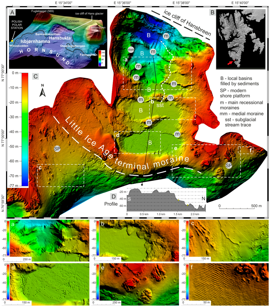
Figure 1.
(A) Study area, a combination of the bathymetric model and DTM (source: S0 Terrengmodell, Norwegian Polar Institute, Tromsø, Norway, Creative Commons); (B) location of the study area in Svalbard; (C) seabed morphology of Isbjørnhamna and Hansbukta Bays in Hornsund Fjord; (a) recessional moraines eroded (overridden) during the glacier advance; (b) tongues from underwater mudslides over fine-grained seafloor; (c) seabed with mass-movement landforms; (d) pockmarks formed by thermogenic gases; (e) N–S cracked exposed bedrock mounds (amphibolites and quartzites) [43]; (f) symmetrical megaripples on fine seabed sediments; (D) bathymetric profile along indicated black line.
Isbjørnhamna and Hansbukta (the latter separated from the former by Baranovskiodden Cape) contain a very clear record of stagnation and areal deglaciation stages of the Hans Glacier. Underwater hills and flat-bottomed basins occur alternately in the longitudinal profile running from the south to the north (i.e., from the sea to the current edge of the glacier; Figure 1D).
In the former case, those are recessional moraines defining the stages of a relative stability of the Hans Glacier’s terminus. The spaces between moraines reflect lack of moraine accumulation, i.e., stages of the glacier retreat. Basins are filled with mineral material coming from the melted ice, flowing in from the fjord and the mainland, and displaced by gravity from abrasively damaged elevations of the underwater moraines. Apart from the local altitude differences, the profile subsides toward the contemporary terminus of the Hans Glacier.
The seabed of the Hansbukta is a confined, arched shallow area extending in the north-westerly direction. On the basis of the ice-sheet ranges determined using a photogrammetric method [5], the elevation can be interpreted as a terminal moraine of the Hans Glacier’s final advance during the Little Ice Age and the glacier extent till the year 1900. As in the case of other Svalbard glaciers, the advance lasted until the 1930s [44,45]. The terminal moraine has the greatest height and volume compared to all other underwater moraines found in the study area. We believe that the ridge of the moraine, levelled by erosion and rising to ca. 10 m below the sea surface, represents a barrier confining the two bays.
The lowermost areas are located at the contemporary Hans Glacier’s terminus, i.e., at a depth of ca. 75 m below the sea surface. These areas were exposed from under the ice during the last 20 years and have not yet been covered with a layer of deposits. Therefore, this level defines the approximate performance of the glacial erosion by the Hans Glacier. The picture of forms connected with the glacier activity is completed with subglacial meltwater channels and elevations originated as a result of crevice accumulation (eskers).
The morphology of the study area is complemented by a rich inventory of smaller bottom forms. The underwater slopes are strongly transformed by slope movements (mass wasting), including submarine mudslides and flows. Their presence is closely related to the slope of the bottom. As a result of slope movements, systems of small ridges and tongues developed and settled on the flat bottom.
Surfaces built of fine-grained material, located within the range of wind-generated waves or ocean currents, are diversified by regular depositional forms—megaripples. Pockmarks, i.e., semicircular, small (0.5 m deep) basins developed as a result of exposure to thermogenic gases, are even more widespread [46,47].
The seafloor morphology of Isbjørnhamna and Hansbukta Bays in the Hornsund Fjord is well described by the basic morphometric parameters of the area, calculated for a moving square window with a side length of 70 m and overlapping of 90%.
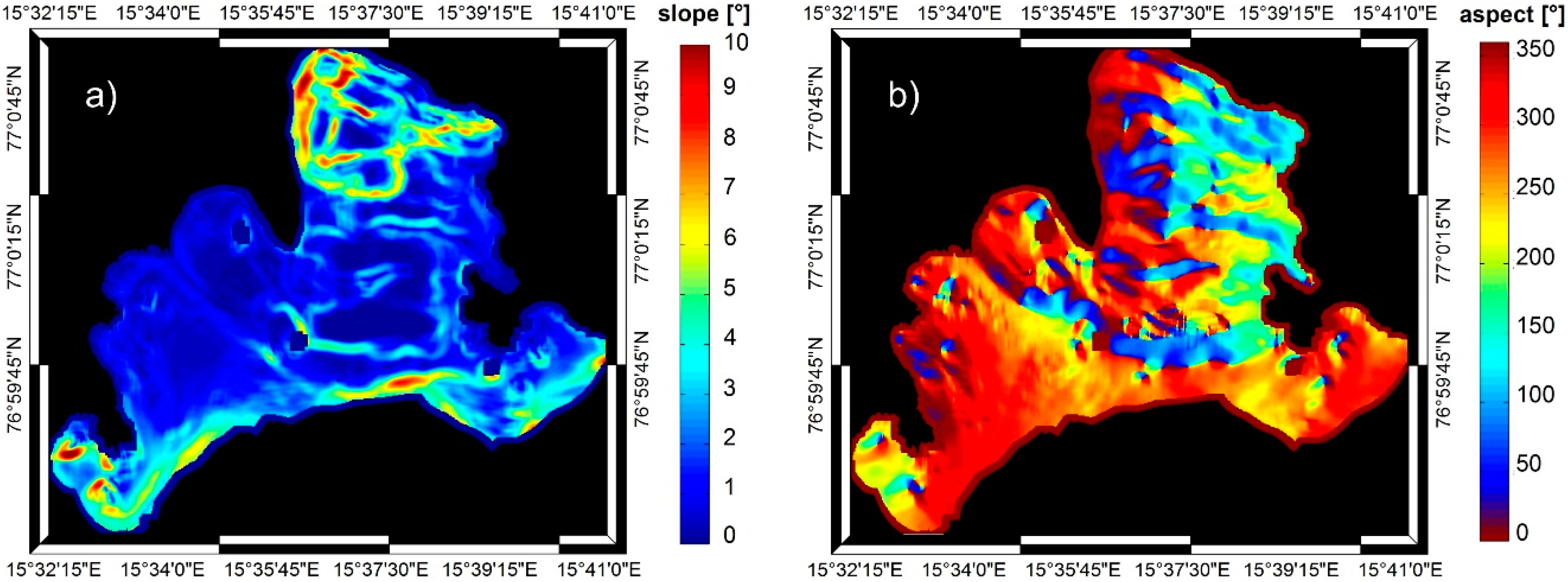
A large window area allows separation of large areas with similar characteristics. A high overlapping value results in a high resolution of the output image. Figure 2a presents slope and Figure 2b—aspect, while Figure 3 shows hypsometric curves. There is a difference between the curve calculated for the inclined surface (red line) and the curve calculated for the detrended surface (blue curve), which illustrates the variability of height due to the presence of morphological forms, without taking into account the inclination of the continental slope. The slope shows the range of the main morphological forms of the bottom and, in particular, the main recessional moraines, while the aspect indicates the directions of their inclination.
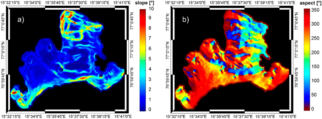
Figure 2.
(a) Slope of the seafloor; (b) aspect of the bay’s seafloor, parameters calculated in a moving window of 70 × 70 m dimensions and overlapping by 90%.

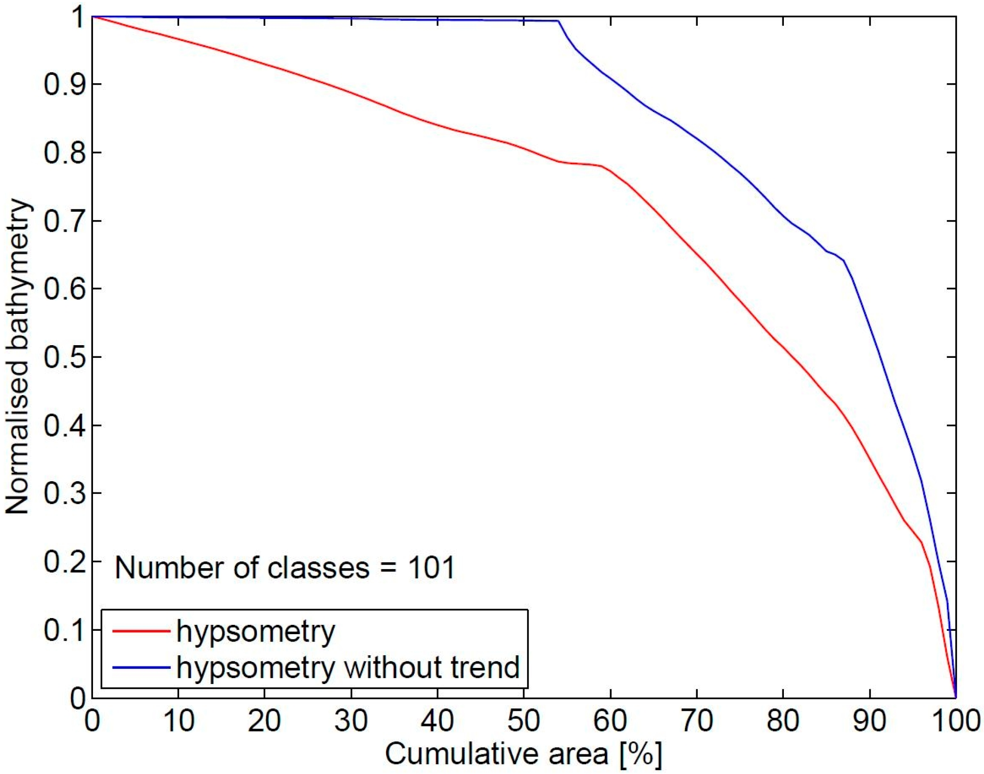
Figure 3.
Hypsometric curves calculated for the inclined surface (red line) and detrended surface (blue line).
The hypsometric curve gently descends to a value equal to 60% of the deepest depth, representing the shallow seabed areas, whereas 40% of the surface is situated within local basins filled with sediments (Figure 1b)—the red line. The hypsometric curve for the detrended surface has a different course—the blue line. In this case, 54% of the surface has approximately the same height in relation to the average depth and corresponds to the flat regions (the map in Figure 1, B and SP areas), and 46% of the area is distinguished by a great relative depth.
3. Method of Bathymetric Data Analysis
The parametrization of the Hansbukta bathymetric DEM required calculations on the matrix of x, y data from the generated terrain model with a horizontal resolution of 0.5 m in the projected Coordinate Reference System of WGS 84/UTM 33N.
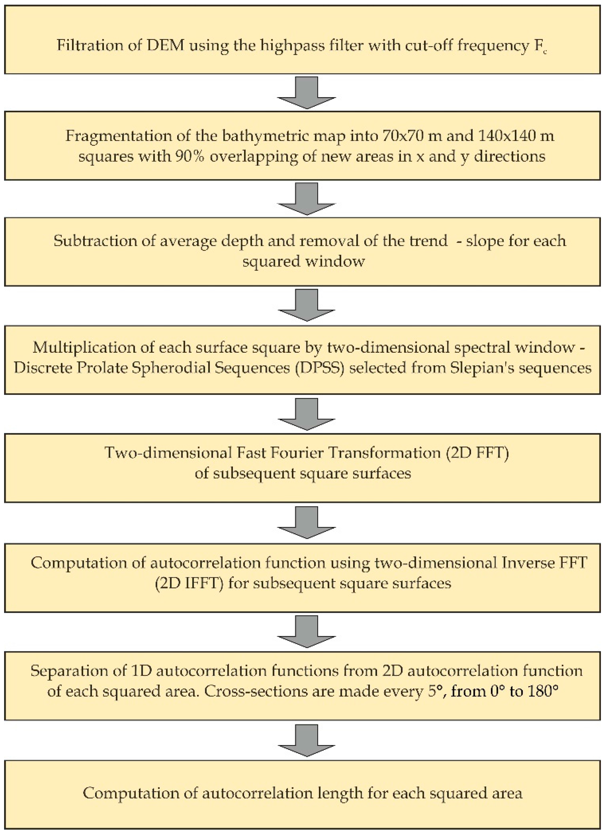
In order to create a map with the distribution of autocorrelation length values on the digital bathymetric model, two square windows were defined with a side length of 70 m and 140 m, respectively. Two windows were selected due to the fact that DEM parameters had to be calculated for two spatial scales. The window moved to the right over the DEM in each subsequent row so as to partially overlap with its previous position. To obtain the spatial distribution of parameters with high resolution, 90% overlapping was applied. Each of the defined squares was multiplied by the three-dimensional Slepian function [48] to remove the effect of spectral leakage, and then a value of average surface inclination (trend) was subtracted. The autocorrelation length for subsequent square windows was calculated using the Wiener–Khinchin theorem to the power spectral density obtained through the Fourier analysis [42,49,50,51]. The results of the thus defined operation for each window was a two-dimensional autocorrelation function, normalized to the maximum value. This was followed by the determination of autocorrelation length equal to a distance Ar, which corresponds to the autocorrelation value equal to e−1.
The Fourier transform F(x) of the stationary random process is defined as follows [49,50]:
where:
- ,
- —angular frequency,
- —frequency [Hz],
- —Fourier transform, i.e., a function of frequency,
- —function of time. To analyse the bottom surface, changes over time should be replaced by spatial changes.
The autocorrelation function was defined as follows [42]:
where:
- —total time of observations,
- —function of time in place t,
- —function of time shifted by a time-step τ.
According to the Wiener–Khinchin theorem, power spectral density can be obtained through the Fourier transformation of the autocorrelation function [49,50]:
and the autocorrelation function is equal to inverse Fourier transformation of power spectral density:
where:
- —the autocorrelation function,
- —power spectral density.
The Two-dimensional Fast Fourier Transformation [52,53,54] defines the spectrum as:
where:
- Kx, Ky—spatial frequencies, values of wave vectors in x, y [m−1] directions,
- —corrugated surface, for which the spectrum is calculated,
- —distance in the directions.
The two-dimensional autocorrelation function was obtained in the calculations conducted in the moving window:
where:
- —two-dimensional power spectral density,
- —lag in the x and y directions.
The autocorrelation function determines the extent to which a given term in a data series depends on the preceding terms in the time series while comparing a given element of the signal with an element of the same signal shifted by one lag (step) τ (a spatial lag in the case of seafloor analysis). Autocorrelation provides information on typical periods and frequencies in the record. The autocorrelation function divided by the spatial scale of oscillations provides normalized values ranging from −1 to 1 (Equation (2)). Autocorrelation values close to 1 reflect a strong positive correlation, which means that an increase in the value of the analysed function f(x) is associated with an increase in the expected value f(x + τ). Values close to −1 indicate a strong negative correlation and an increase in the analysed value, which involves a decrease in the expected value. Values close to 0 indicate a lack of any relationships between the function and its copy shifted by τ.
The highest value of the autocorrelation function is obtained in the absence of lag τ, i.e., when a perfect similarity occurs between the function and its copy. If the considered function is constant, its values do not change and the value of autocorrelation for each lag is 1. For a periodic function with a period T, hereinafter referred to as wave, the value of the autocorrelation function decreases with the increasing lag τ until the lag is equal to half the wavelength. From this point, the value of autocorrelation reaches the first minimum and begins to increase. The maxima of the autocorrelation function are repeated for the values equal to a multiple of the wavelength [55].
The schematic description of the algorithm of autocorrelation length computation is shown in Figure 4.
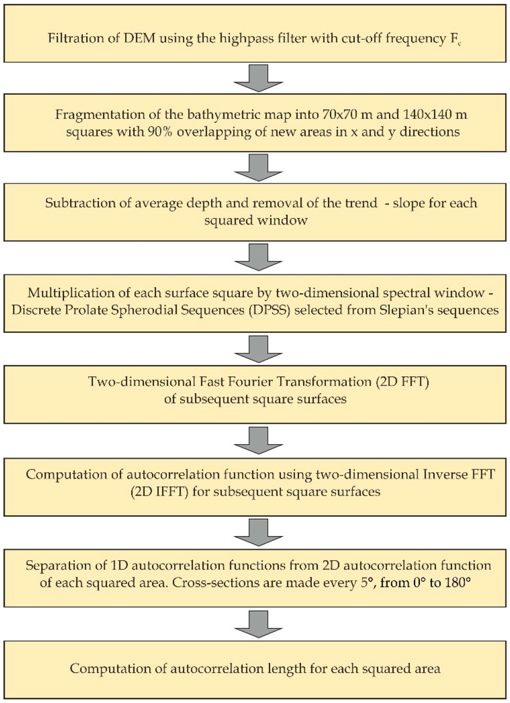
Figure 4.
Flowchart of the autocorrelation length computation.
The value of the autocorrelation function in the moving window is dominated by the spatial dimension close to the size of the moving window. Calculations of the autocorrelation function result in values corresponding to the distribution of ridges and valleys on the seafloor at a given spatial scale, burdened with an error resulting from the limitations of the measurement window. To obtain the actual distribution of the terrain roughness, the bathymetric image should be subjected to a high-pass filter [56]. The objective of the process is to obtain a distribution of terrain roughness with wavenumbers Kxy ranging from the maximum values, resulting from the spatial resolution of the input image, to the lowest values which will not introduce wave structures of a size close to the window size into the output image. Therefore, a high-pass filter was used with a filtration limit close to the maximum.
To test the calculation algorithm, an artificial sinusoidal surface was built (Figure 5a) and a two-dimensional autocorrelation function was calculated (Figure 5b). Next, cross-sections of the autocorrelation function were made every 5° from the central point to the edge of the window, through the determination of one-dimensional autocorrelation functions (Figure 5c). The autocorrelation length, Ar, is a distance, which corresponds to the normalized value of the autocorrelation function equal to e−1 = 0.3697 [12]. Values of the autocorrelation length should not be directly compared with the size of morphological forms. In the next step, the autocorrelation length values for each cross-section (Figure 5d) were read and averaged for the whole window. The above-described algorithm was applied to the window moving over the DEM and the calculated values of the autocorrelation length were presented on the output map (Figure 6 and Figure 7).
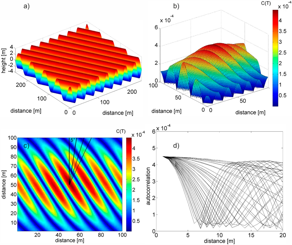
Figure 5.
(a) Artificially generated surface with a regular, sinusoidal shape and spatial frequency of 0.033 m−1; (b) the autocorrelation function for the sinusoidal surface in the moving window with a side length of 100 units; (c) determination of cross-sections through the 2D autocorrelation function, every 5°; (d) cross-sections of the 2D autocorrelation function in the window with a side length of 100 units, every 5°.

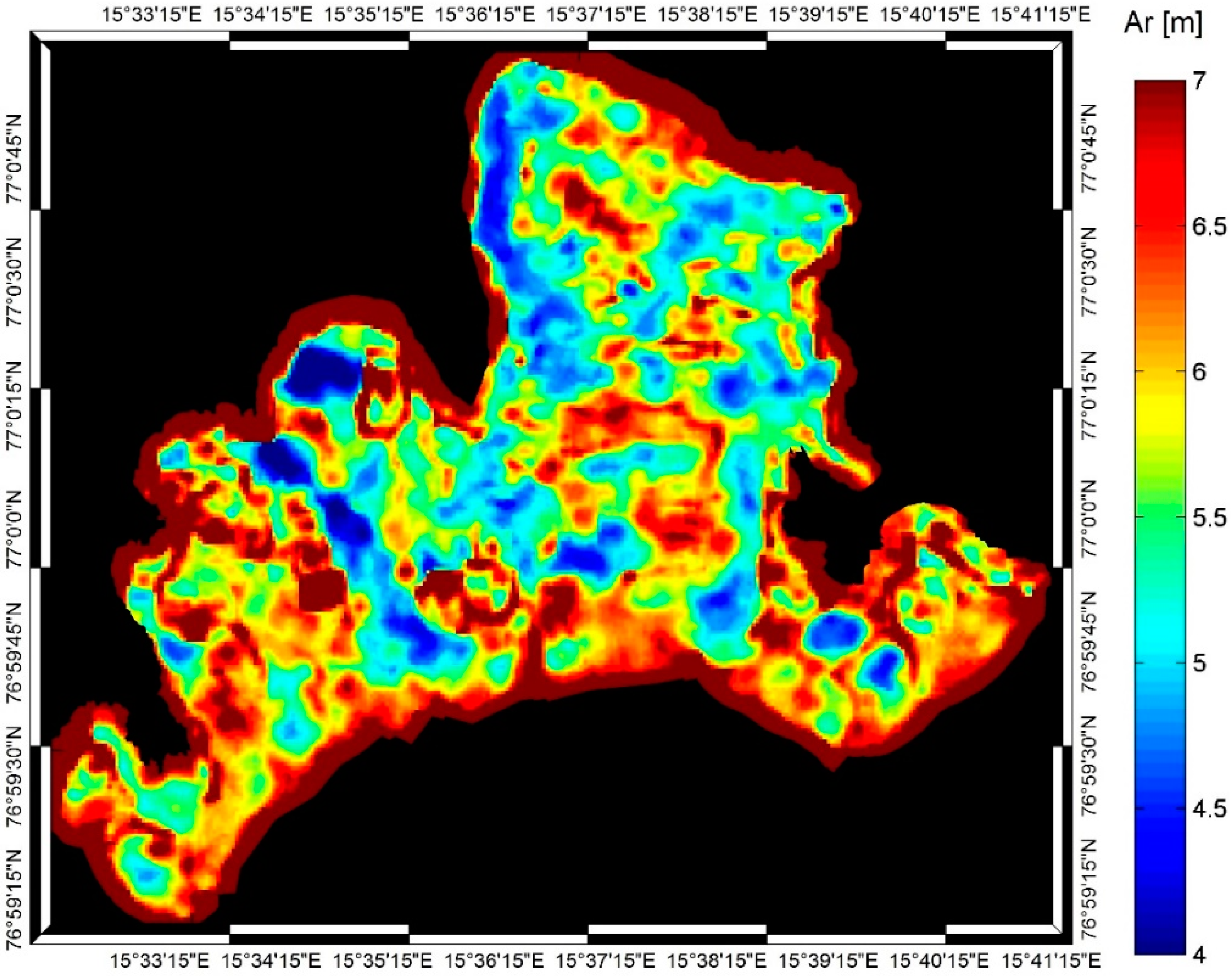
Figure 6.
The autocorrelation length describing the terrain roughness with a spatial scale of 2 m–98 m, for DEM with a step of d = 1.0 m and the moving window with a side length of 140 m and 90% overlapping.

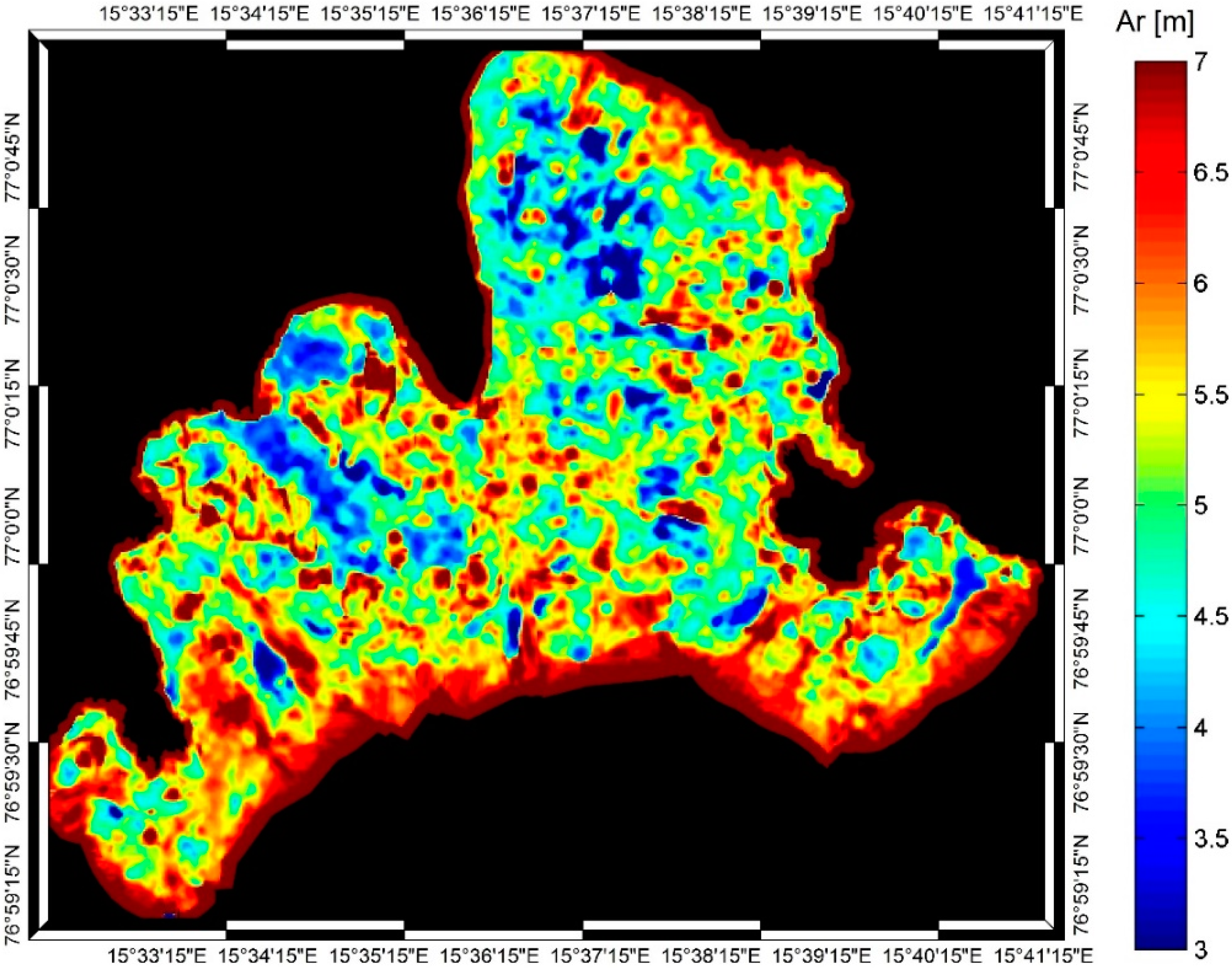
Figure 7.
The autocorrelation length describing the terrain roughness with a spatial scale of 1–49 m, for DEM with a step of d = 0.5 m in a moving window with a side length of 70 m and the overlapping of 90%.
If the surface has a low spatial frequency, the value of autocorrelation length is high. Low frequency is correlated with slower changes in the height along with the increasing distance, and hence small roughness [12]. The value of the autocorrelation length reflects the rate of changes in the height with the increasing distance.
4. Results
Calculations of the autocorrelation length for the DEM in Isbjørnhamna and Hansbukta Bays in the Hornsund Fjord resulted in the distribution maps of the autocorrelation length values: (i) for the input data with a sampling step of 0.5 m, where the autocorrelation length describes the terrain roughness on the spatial scale ranging from 1.0 m to 49.0 m; (ii) for the input data with a sampling step of 1.0 m, where the autocorrelation length describes the terrain roughness on the spatial scale ranging from 2.0 m to 98.0 m.
On the basis of tests carried out on the artificially generated digital surfaces, it has been determined that in order to remove a spatial dimension of the size close to the size of a moving window from the image, a filter with a limit of at least seven times higher than a spatial frequency should be used, understood as 1/length of the scale of this dimension.
A high-pass filter was used for the image with the highest resolution, defining damping below the spatial frequency:
where:
- —cut-off frequency of a high-pass filter,
- —spatial frequency of 49 m long roughness, which is equal to .
The measured area of the bay’s bottom is not rectangular and during visualization of the bathymetry, the area was inscribed into a rectangle, while the value of 0 was assigned to sites with unknown bathymetry. In the process of filtering and calculation of autocorrelation and its length, these sites were also analysed, however, they should not be included in the interpretation of the results. The statistic was not calculated along the peripheries of the study area; the output map is smaller and consists of a smaller number of points dependent on the size of the moving window.
The high spatial resolution image was obtained, which shows the distribution of autocorrelation length values (Figure 6 and Figure 7).
Figure 6 presents the distribution of autocorrelation length calculated for the DEM with a resolution of d = 1 m. The data variability at scales below 2 m tend to be dominated by various forms of noise (acoustic, motion sensor, GPS [20]), so the analysis was deliberately designed to ignore these short wavelengths by starting the Fourier Transform at a 2 m wavelength. As a result, small morphological structures were not included in the analysis and, at the same time, a significant part of artefacts and noise (measurement errors) was removed. The picture of autocorrelation length distribution reflects the roughness of a spatial scale ranging from 2 m to 98 m. Values of the autocorrelation length are calculated in the moving window with a side length of 140 m, hence the resolution of the output image is much lower compared to the calculations in the window with a 70 m side (Figure 7). Nevertheless, this allows the determination of larger surfaces with similar properties. Therefore, local basins filled with sediments (B in Figure 1) have a long autocorrelation length. Elevations of the recessional moraines on a spatial scale of 2 m–98 m are undulating areas distinguished by a short autocorrelation length.
The most intensive sedimentation takes place at the glacier terminus where detached ice fragments are melting. Most of the terrigenous material is deposited in sedimentary basins located close to the glacier terminus. Thawing of large rock fragments falling into soft bottom sediments largely contributes to the development of surface forms that are called dropstones [57,58]. The autocorrelation length has low values for local sediment-filled basins with pockmarks.
Exposed bedrock mounds built of hard and felsic, eroded, magmatic, igneous rocks [43] have a short autocorrelation length. Smooth surfaces between bedrock mounds are covered with sediments and have a high value of the studied parameter.
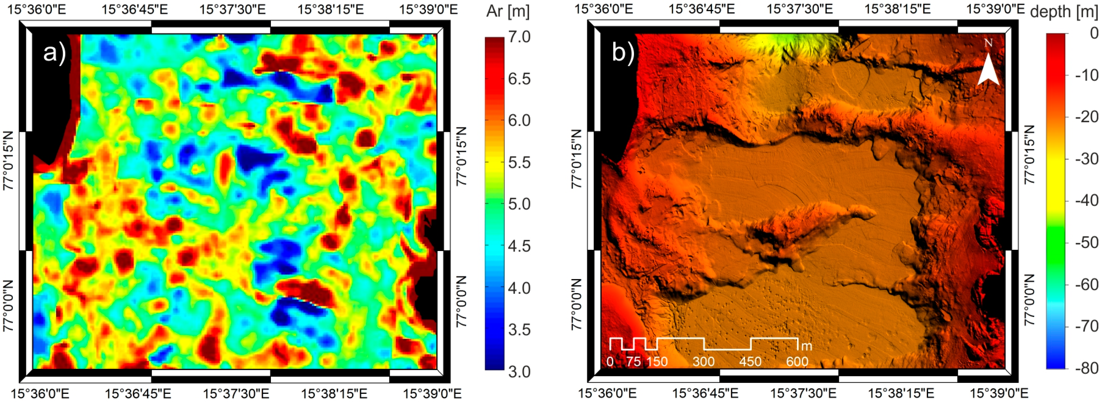
Figure 6 shows values of the autocorrelation length calculated from the input data with a resolution of d = 0.5 m. In the northern part of the study area, local basins filled with sediments are located in the closest proximity of the glacier terminus (B in Figure 1C). Their surface is covered with minor roughness and linear artefacts resulting from measurement errors, and the autocorrelation length has low values. Elevations of recessional moraines occur between sedimentary basins. Their surface is smoother compared to the fjord’s bottom covered with artefacts and small roughness, hence long autocorrelation length was determined here (Figure 8a,b).
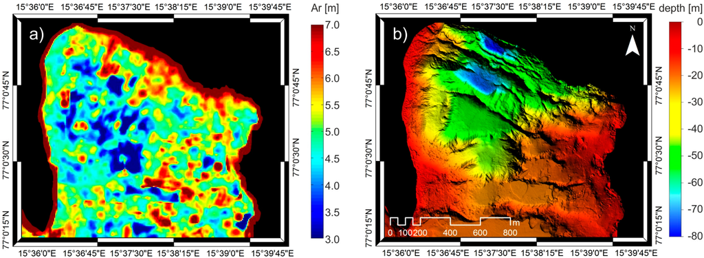
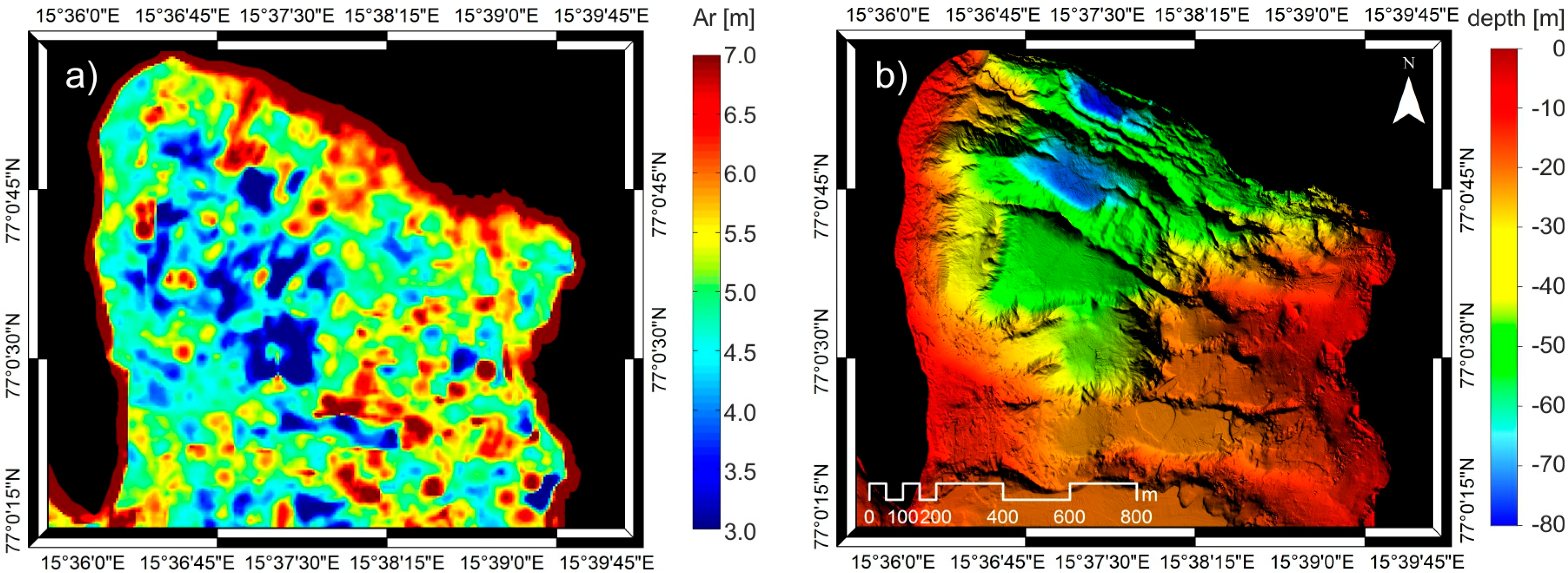
Figure 8.
Detailed maps of the bottom of Isbjørnhamna and Hansbukta Bays in the Hornsund Fjord, which compare the autocorrelation length (a parameter describing the terrain roughness with a spatial scale in the range of 1–49 m, for DEM with a step of d = 0.5 m in the moving window with a side length of 70 m and 90% overlapping) with the bathymetry of the area; (a) the autocorrelation length and (b) seafloor morphology of the same area with basins filled with sediments and recessional moraines.
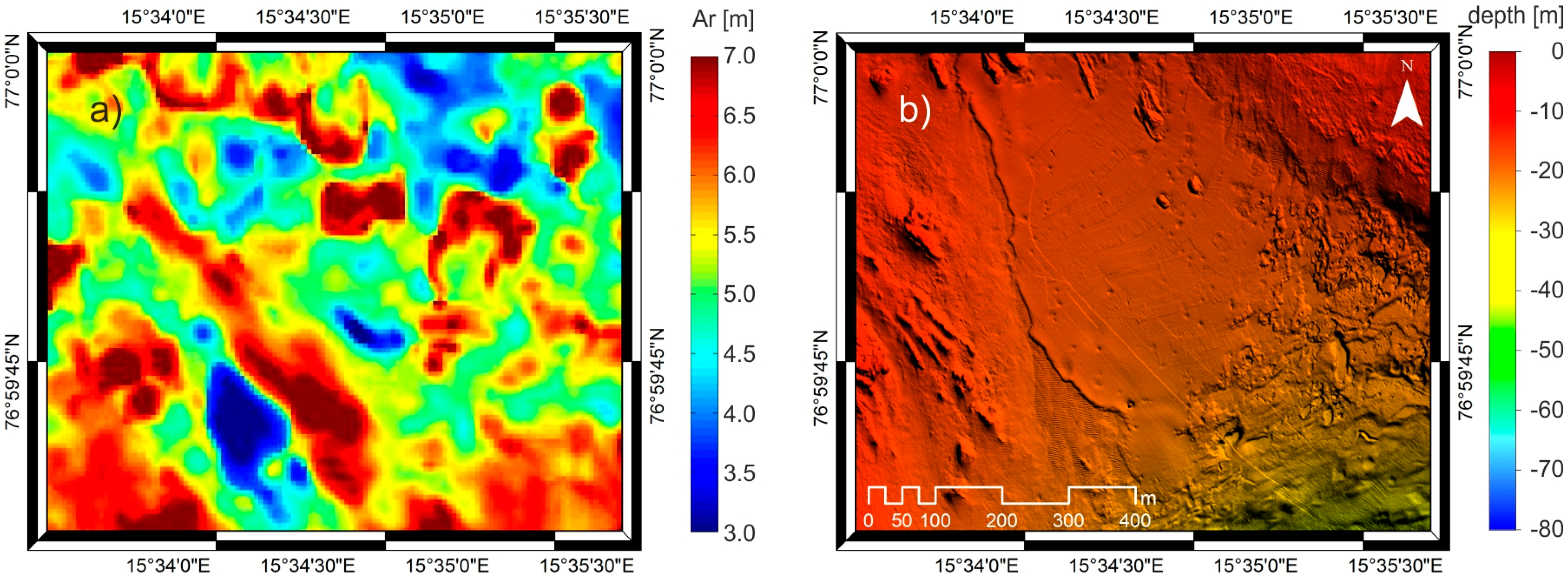
Pockmarks occur in some of the local basins filled with sediments. The value of the autocorrelation length ranges from 4 m to 6 m. Tongues of underwater mudslides, occurring in the central part of the study area, are characterised by relatively high values of the autocorrelation length, ranging from 4.5 m to 6.5 m (Figure 9a,b).

Figure 9.
Detailed maps of the bottom of Isbjørnhamna and Hansbukta Bays in the Hornsund Fjord, which compare the autocorrelation length (a parameter describing the terrain roughness with a spatial scale in the range of 1–49 m, for DEM with a step of d = 0.5 m in the moving window with a side length of 70 m and 90% overlapping) and the bathymetry of the area; (a) value of the autocorrelation length and (b) seafloor morphology in the place with characteristic tongues of underwater mudslides and pockmarks.
In the south-eastern part of the area, exposed bedrock mounds built of amphibolites and quartzites are found. Cracked and eroded hard rocks form irregular surfaces. The bathymetric image shows peaks of exposed bedrock mounds obscured by artefacts resulting from measurement errors; they also form a rough surface—that is why places with rocks are characterized by a short autocorrelation length. Exposed bedrock mounds suppress the energy of waves, which results in a smooth cover of sediment between sharp rocks, which is reflected in high values of the parameter, i.e., above 6 m. The wave motion formed megaripples in the sediment cover east and west of the exposed bedrock mounds—these sites are characterized by a particularly short autocorrelation length, close to 3.5 m (Figure 10a,b).
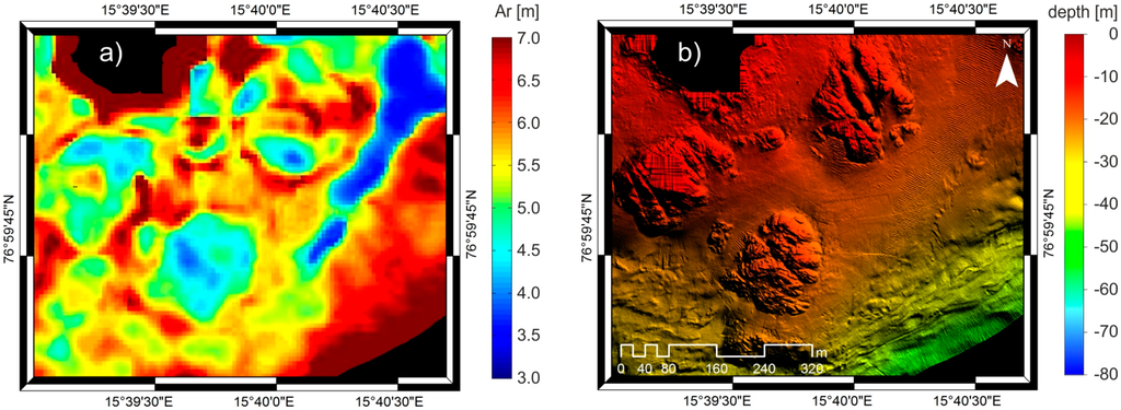
Figure 10.
Detailed maps of the bottom of Isbjørnhamna and Hansbukta Bays in Hornsund Fjord, which compare the autocorrelation length (a parameter describing the terrain roughness with a spatial scale in the range of 1–49 m, for DEM with a step of d = 0.5 m in the moving window with a side length of 70 m and 90% overlapping) and the bathymetry of the area; (a) value of the autocorrelation length and (b) seafloor morphology in the place with exposed bedrock mounds and megaripples.
Seabed with mass-movement landforms are distinguished by very longautocorrelation length, i.e., almost 7 m, while places with megaripples have short—below 4.5 m (Figure 11a,b).

Figure 11.
Detailed maps of the bottom of Isbjørnhamna and Hansbukta Bays in Hornsund Fjord, which compare the autocorrelation length (a parameter describing the terrain roughness with a spatial scale in the range of 1–49 m, for DEM with a step of d = 0.5 m in the moving window with a side length of 70 m and 90% overlapping) and the bathymetry of the area; (a) value of the autocorrelation length and (b) seafloor morphology in the place with mass-movement landforms and megaripples.
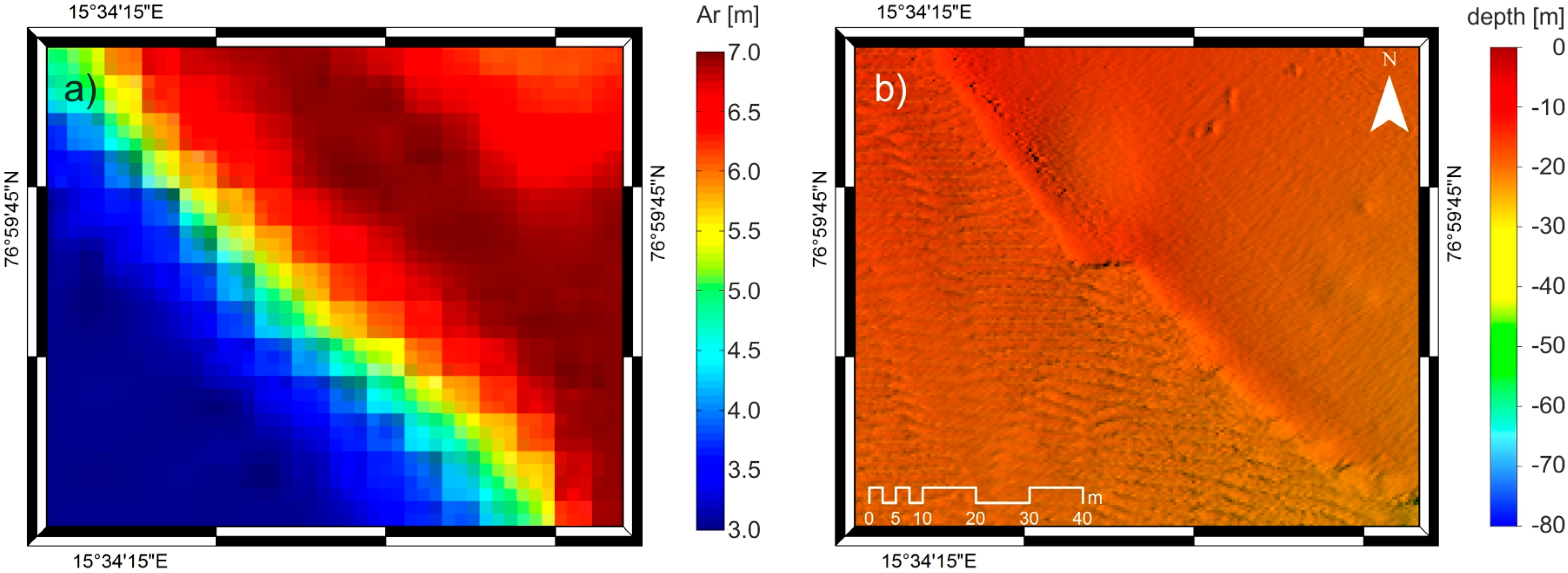
An example of the autocorrelation length estimation is presented in Figure 12, which shows the bathymetric map magnified at a level close to the horizontal resolution of the gridded bathymetry, i.e., 0.5 m. Megaripples of 2.5–3.0 m and a flat seafloor area are visible in the DEM of a small rectangular, 108 × 89 m area selected from the central part of Figure 11 (Figure 12b). Values of the autocorrelation length vary from 3 to 7 m depending on the roughness of the seabed (Figure 12a). The figures make it possible to distinguish features of size down to 2.5 m.

Figure 12.
Autocorrelation length (a) and DEM of 108 × 89 m area selected from the central part of Figure 11 (b). The figures make it possible to distinguish geomorphological forms of size down to 2.5 m.
5. Discussion
Both tests conducted on the artificially generated digital surface of the bottom and the calculations on the Hansbukta DEM indicate that the autocorrelation length performs well in the description of surface corrugation. The parameter properly describes the morphological features of the bottom. The computation algorithms for the distribution of autocorrelation length values, despite the complicated procedure, are much faster compared to the calculations carried out on the basis of the definition (Equation (2)). The calculation of the autocorrelation length in the moving window resulted in the spatial distribution of this parameter for the entire seafloor of the study area. High values correspond to relatively flat areas such as flat sandy bottoms and depressions filled with sediments, while low values correspond to considerably undulating areas such as exposed bedrock mounds, ripple marks or terminal moraines. The autocorrelation length allows to distinguish morphological structures of the bottom.
Table 1 presents the calculated statistical parameters which describe the main morphological forms of Hansbukta bottom.

Table 1.
Values of statistical parameters for the main morphological forms of Hansbukta bottom.
The output map presenting the distribution of the autocorrelation length values provides information on the undulation of the area in a specific spatial scale. Selection of scale parameters is determined by: (i) resolution of the input data—the bathymetry based on points located at 0.5 m intervals (Nyquist frequency) does not include land forms shorter than 1 m and the bathymetry based on points located at 1 m intervals does not include forms with a length below 2 m; (ii) a filter suppressing low frequencies; a filter should remove components with a length greater than half the length of the moving window so the information on the length of low-frequency components is not dominated by the autocorrelation values, which results from Nyquist’s frequency. A high-pass filter with a given spatial frequency limit (seven times higher compared to the spatial frequency of the roughness scale intended for removal) was used in the analysis.
It is also important to note that the use of a moving window, which partially overlaps with its previous location, considerably improved the resolution of the output map. The large size of the moving window (70 m and 140 m) contributed to the deterioration of the image resolution, but allowed for the minimization of the autocorrelation error resulting from calculations for a window with a smaller size.
The algorithm can work for windows of size ranging from 38 × 38 up to 140 × 140 points of bathymetry. Estimation of the autocorrelation for short series results in a considerable calculation error. Therefore, it is assumed that the calculation of the autocorrelation length is always in a window containing 140 × 140 points. To calculate the autocorrelation length in a larger window, the algorithm uses a DEM of a lower resolution. A 70 m × 70 m window was used to calculate the autocorrelation for DEM having a resolution of 0.5 m, and a 140 m × 140 m window—for DEM having a resolution of 1 m. Large square windows of 140 m × 140 m are used to analyse low-frequency spectral components, which build the morphology of the seafloor, however, they lose information on high frequency components. In order to register the signal in digital recording, the frequency must be less than half of the sampling rate. If the frequency is higher, it cannot be observed in the analysed signal. The size of the overlapping windows has no effect on the correctness of the calculation of the autocorrelation and its length, however it has a significant impact on the resolution of the resulting image. Image resolution is proportional to the square of the overlapping quantity.
Sporadic DEM artifacts are usually an effect of measurement errors in a short autocorrelation length and do not result from the seabed roughness. We are aware that the results presented in this paper do not directly reflect the features of geomorphological forms but they contain important information on the bottom roughness. The presented parameter also indirectly carries information about the processes shaping the bottom e.g., deglaciation, sedimentation, bottom currents and mass movements.
In this study, we conducted a validation of the autocorrelation length computation procedure by comparing the obtained results in the form of spatial distribution maps with high resolution DEM for the study area. DEM has a high spatial resolution of 0.5 m and therefore, in this case, the comparison of computed values of the autocorrelation length with the bathymetric model is a reliable method of validation.
According to the Nyquist theorem, the largest scale of irregularities in the analysis is half the length of the moving window (size of the moving window affects the size of morphological forms, which are considered in the analysis). The smallest scale of irregularities which affect the autocorrelation is two times higher than a distance between the measurement points (density of the sampling determines the highest frequency present in the digital image). Registration of the bottom at low resolution makes it impossible to study small forms, because they do not occur in the digital terrain model.
Many authors have attempted to describe a rough surface using fractal geometry, wavelet and statistical analysis. Fractal dimension used in the description of a given area yields high values in heterogeneous places and low values in flat areas ranging from 2 to 3 [34]. It was used in the description of the seabed undulation on the continental slope to identify benthic habitats. The above method and wavelet analysis enabled the authors to fairly accurately distinguish coral colonies protruding from a relatively flat and soft bottom. While studying the topography of Mars, Aharonson et al. [59] used a parameter referred to as “decorrelation length”, which is equal to a distance corresponding to half of the autocorrelation function’s value. With the use of this and other parameters, e.g., a median of slopes, the authors conducted a very accurate detection of meteorite craters on the planet’s surface.
The autocorrelation length, described by Ogilvy J.A. [12] and used in the description of the seabed roughness, yields interesting results. It is an efficient method to identify areas covered with miscellaneous seabed forms, in particular when allowing for their length in a cross-section. Ripple marks and sand waves may represent a good example, which, despite a similar structure, have different values of the autocorrelation length as a result of their varying size.
The obtained values of the autocorrelation length for the seabed surface in Hansbukta comprehensively describe the terrain roughness and the scale of the glacial bay seafloor roughness, assigning its values to various morphological structures occurring in the surveyed sea area.
6. Conclusions
A new terrain analysis system for parameterization of the seafloor roughness was developed and successfully tested. The new algorithm of the autocorrelation length permits the differentiation of morphological structures of uneven seafloor surfaces.
The obtained results of the autocorrelation length defining the surface roughness can be directly referred to bathymetric data and morphology of the bottom in Isbjørnhamn and Hansbukta Bays. The output map created with the use of a moving 140 m × 140 m window shows an alignment between high values of the autocorrelation length and regions with a flat seabed topography (local sedimentary basins between the underwater moraine ridges and fragments of the seabed covered with deposit between Wilczekodden and Baranovskiodden). Terminal (recessional) moraine ridges are relatively correctly represented, this time with low values of the autocorrelation length. This parameter differentiates the largest moraine—the terminal moraine from LIA (Little Ice Age)—and well reflects the heterogeneous morphology of its surface. The lowest values of the autocorrelation length are reserved for a highly diversified shore zone with runoffs of deposits and sometimes outcrops of monolithic rocks.
When calculating the autocorrelation length for a moving 70 m × 70 m window, high values of the autocorrelation were obtained for flat seabed areas and lowest values for areas with small landforms (ca. 2.5–8 m). The result of the calculations is strongly correlated with local changes in the roughness.
We have designed and tested a method of describing the seafloor roughness by the autocorrelation length. The calculation of the autocorrelation length in the moving window resulted in the spatial distribution of this parameter for the entire seafloor of the study area. Even though the ranges of the autocorrelation length values partially overlap for different morphological forms, they properly represent the distribution and limits of the seafloor structures.
The presented method of calculating the autocorrelation parameter of the seafloor in the region of the glacier’s retreat facilitates the identification and classification of geomorphological forms, potentially providing information about the changes in the seabed structure caused by ice melting in the Arctic.
Acknowledgments
The authors were supported by the Polish National Science Centre grant 2011/03/B/ST10/04275.
Author Contributions
J.T. conceived and designed the study; J.T., K.T., J.N. performed the algorithm; K.T., J.T. performed calculations, analysed and described results; M.K. recognize and described geomorphology of the studied area.
Conflicts of Interest
The authors declare no conflict of interest.
References
- Stroeve, J.; Maslowski, W. Arctic sea ice variability during the last half century. In Climate Variability and Extremes during the Past 100 Years; Brönnimann, S., Luterbacher, J., Ewen, T., Diaz, H.F., Stolarski, R.S., Neu, U., Eds.; Springer: Dordrecht, The Netherlands, 2007; pp. 143–154. [Google Scholar]
- Maslowski, W.; Kinney, J.C.; Higgins, M.; Roberts, A. The future of Arctic sea ice. Annu. Rev. Earth Planet. Sci. 2012, 40, 625–654. [Google Scholar] [CrossRef]
- Grabiec, M.; Jania, J.; Puczko, D.; Kolondra, L.; Budzik, T. Surface and bed morphology of Hansbreen, a tidewater glacier in Spitsbergen. Pol. Polar Res. 2012, 33, 111–138. [Google Scholar] [CrossRef]
- Błaszczyk, M.; Jania, J.; Kolondra, L. Fluctuations of tidewater glaciers in Hornsund Fjord (Southern Svalbard) since the beginning of the 20th century. Pol. Polar Res. 2013, 34, 327–352. [Google Scholar] [CrossRef]
- Vieli, A.; Jania, J.; Kolondra, L. The retreat of a tidewater glacier: Observations and model calculations on Hansbreen, Spitsbergen. J. Glaciol. 2002, 48, 592–600. [Google Scholar] [CrossRef]
- Jania, J.; Kaczmarska, M. Hans Glacier—A tidewater glacier in southern Spitzbergen: Summary of some results. In Calving Glaciers: Report of a Workshop, February 28–March 2, 1997, Byrd Polar Research Center, Report nr. 15; Van der Veen, C.J., Ed.; Ohio State University: Columbus, OH, USA, 1997; pp. 95–104. [Google Scholar]
- Ernstsen, V.; Noormets, R.; Hebbeln, D.; Bartholomä, A.; Flemming, B. Precision of high-resolution multibeam echo sounding coupled with high-accuracy positioning in a shallow water coastal environment. Geo Mar. Lett. 2006, 26, 141–149. [Google Scholar] [CrossRef]
- Goff, J.A. A global and regional stochastic analysis of near-ridge abyssal hill morphology. J. Geophys. Res. 1991, 96, 713–737. [Google Scholar] [CrossRef]
- Scott, R.B.; Goff, J.A.; Naveira-Garabato, A.C.; Nurser, A.J.G. Global rate and spectral characteristics of internal gravity wave generation by geostrophic flow over topography. J. Geophys. Res. 2011, 116, 1–14. [Google Scholar] [CrossRef]
- Bhushan, B. Contact mechanics of rough surfaces in tribology: Multiple asperity contact. Tribol. Lett. 1998, 4, 1–35. [Google Scholar] [CrossRef]
- Bass, F.G.; Fuks, I.M. Wave Scattering from Statistically Rough Surfaces, 1st ed.; Pergamon Press Ltd.: Oxford, UK, 1979; p. 540. [Google Scholar]
- Ogilvy, J.A. Theory of Wave Scattering from Random Rough Surfaces; Adam Higler: Bristol, UK, 1991; p. 277. [Google Scholar]
- Godone, D.; Garnero, G. The role of morphometric parameters in Digital Terrain Models interpolation accuracy: A case study. Eur. J. Remote Sens. 2013, 46, 198–214. [Google Scholar] [CrossRef]
- Schimel, A.C.G.; Healy, T.R.; McComb, P.; Immenga, D. Comparison of a Self-Processed EM3000 Multibeam Echosounder Dataset with a QTC View Habitat Mapping and a Sidescan Sonar Imagery, Tamaki Strait, New Zealand. J. Coast. Res. 2010, 26, 714–725. [Google Scholar] [CrossRef]
- Hamilton, L.J.; Mulhearn, P.J.; Poeckert, R. Comparison of RoxAnn and QTC–View acoustic bottom classification system performance for the Cairns area, Great Barrier Reef, Australia. Cont. Shelf Res. 1999, 19, 1577–1597. [Google Scholar] [CrossRef]
- Tegowski, J.; Gorska, N.; Klusek, Z. Statistical analysis of acoustic echoes from underwater meadows in the eutrophic Puck Bay (southern Baltic Sea). Aquat. Living Resour. 2003, 16, 215–221. [Google Scholar] [CrossRef]
- Tamsett, D. Sea-bed characterisation and classification from the power spectra of side-scan sonar data. Mar. Geophys. Res. 1993, 15, 43–64. [Google Scholar] [CrossRef]
- Blondel, P. Textural analysis of sidescan sonar imagery and generic seafloor characterisation. J. Acoust. Soc. Am. 1999, 105, 1206. [Google Scholar] [CrossRef]
- Hamilton, L.J.; Parnum, I. Acoustic seabed segmentation from direct statistical clustering of entire multibeam sonar backscatter curves. Cont. Shelf Res. 2011, 31, 138–148. [Google Scholar] [CrossRef]
- Hughes Clarke, J.E.; Mayer, L.A.; Wells, D.E. Shallow-water imaging multibeam sonars: A new tool for investigating seafloor processes in the coastal zone and on the continental shelf. Mar. Geophys. Res. 1996, 18, 607–629. [Google Scholar] [CrossRef]
- Goff, J.A. Quantative Characterstics of Abyssal Hill Morphology along flow line in the Atlantic Ocean. J. Geophys. Res. 1992, 97, 9183–9202. [Google Scholar] [CrossRef]
- Mitchell, N.C.; Hughes Clarke, J.E. Classification of seafloor geology using multibeam sonar data from the Scotian Shelf. Mar. Geol. 1994, 121, 143–160. [Google Scholar] [CrossRef]
- Goff, J.A.; Jordan, T.H. Stochastic modeling of seafloor morphology: Inversion of Sea Beam data for second-order statistics. J. Geophys. Res. 1988, 93, 13589–13608. [Google Scholar] [CrossRef]
- Goff, J.A. Quantitative classification of canyon systems on continental slopes and a possible relationship to slope curvature. Geophys. Res. Lett. 2001, 28, 4359–4362. [Google Scholar] [CrossRef]
- Goff, J.A.; Tucholke, B.E.; Lin, J.; Jaroslow, G.E.; Kleinrock, M.C. Quantitative analysis of abyssal hills in the Atlantic Ocean: A correlation between inferred crustal thickness and extensional faulting. J. Geophys. Res. 1995, 100, 22509–22522. [Google Scholar] [CrossRef]
- Goff, J.A. Global prediction of abyssal hill root-mean-square heights from small-scale altimetric gravity variability. J. Geophys. Res. 2010, 115, 1–16. [Google Scholar] [CrossRef]
- Herzfeld, U.C. A method for seafloor classification using directional variograms, demonstrated for data from the western flank of the Mid-Atlantic Ridge. Math. Geol. 1993, 25, 901–924. [Google Scholar] [CrossRef]
- Ishimaru, A. Wave Propagation and Scattering in Random Media, 2nd ed.; IEEE Press and Oxford University Press: New York, NY, USA, 1997; p. 574. [Google Scholar]
- Tegowski, J.; Lubniewski, Z. Seabed characterisation using spectral moments of the echo signal. Acta Acust. United Acust. 2002, 88, 623–626. [Google Scholar]
- Mandelbrot, B.B. The Fractal Geometry of Nature; Freeman: San Francisco, CA, USA, 1982; p. 468. [Google Scholar]
- Hastings, H.M.; Sugihara, G. Fractals—A User’s Guide for the Natural Sciences; Oxford University Press: New York, NY, USA, 1993; p. 235. [Google Scholar]
- Malinverno, A. Segmentation of Topographic Profiles of the Seafloor Based on a Self-Affine Model. IEEE J. Ocean. Eng. 1989, 14, 348–359. [Google Scholar] [CrossRef]
- Qian, Z.W. Wave scattering on a fractal surface. J. Acoust. Soc. Am. 2000, 107, 260–262. [Google Scholar] [CrossRef] [PubMed]
- Fox, C.G.; Hayes, D.E. Quantitative methods for analyzing the roughness of the seafloor. Rev. Geophys. 1985, 23, 1–48. [Google Scholar] [CrossRef]
- Wilson, M.F.J.; O’Connell, B.; Brown, C.; Guinan, J.C.; Grehan, A.J. Multiscale terrain analysis of multibeam bathymetry data for habitat mapping on the continental slope. Mar. Geod. 2007, 30, 3–35. [Google Scholar] [CrossRef]
- Rippin, D.M.; Bamber, J.L.; Siegert, M.J.; Vaughan, D.G.; Corr, H.F.J. Basal conditions beneath enhanced-flow tributaries of Slessor Glacier, East Antarctica. J. Glaciol. 2006, 52, 481–490. [Google Scholar] [CrossRef]
- Graham, A.G.C.; Larter, R.D.; Gohl, K.; Hillenbrand, C.-D.; Smith, J.A.; Kuhn, G. Bedform signature of a West Antarctic palaeo-ice stream reveals a multi-temporal record of flow and substrate control. Quat. Sci. Rev. 2009, 28, 2774–2793. [Google Scholar] [CrossRef]
- Hoffman, R.; Krotkov, E. Terrain Roughness Measurement from Elevation Maps. Proc. SPIE 1989, 1195, 104–114. [Google Scholar]
- Hollaus, M.; Höfle, B. Terrain Roughness parameters from full-waveform airborne LIDAR data. In Proceedings of the ISPRS TC VII Symposium—100 Years ISPRS, Vienna, Australia, 5–7 July 2010; Volume XXXVIII, pp. 287–292.
- Doneus, M.; Briese, C.; Fera, M.; Janner, M. Archaeological prospection of forested areas using full-waveform airborne laser scanning. J. Archaeol. Sci. 2008, 35, 882–893. [Google Scholar] [CrossRef]
- Aubrecht, C.; Höfle, B.; Hollaus, M.; Köstl, M.; Steinnocher, K.; Wagner, W. Vertical roughness mapping—ALS based classification of the vertical vegetation structure in forested areas. In Proceedings of the ISPRS TC VII Symposium—100 Years ISPRS, Vienna, Australia, 5–7 July 2010; Volume XXXVIII, pp. 35–40.
- Beauchamp, K.G. Signal Processing: Using Analog and Digital Techniques; Allen and Unwin: London, UK, 1973; p. 584. [Google Scholar]
- Czerny, J.; Kieres, A.; Manecki, M.; Rajchel, J. Geological Map of the SW Part of Wedel Jarlsberg Land Spitsbergen, 1:25 000; Institute of Geology and Mineral Deposits, University of Mining and Metallurgy: Cracow, Poland, 1992. [Google Scholar]
- Svendsen, J.I.; Mangerud, J. Holocene glacial and climatic variations on Spitsbergen, Svalbard. Holocene 1997, 7, 45–57. [Google Scholar] [CrossRef]
- Lønne, I.; Lysa, A. Deglaciation dynamics following the Little Ice Age on Svalbard: Implications for shaping of landscapes at high latitudes. Geomorphology 2005, 72, 300–319. [Google Scholar] [CrossRef]
- Damm, E.; Mackensen, A.; Budéus, G.; Faber, E.; Hanfland, C. Pathways of methane in seawater: Plume spreading in an Arctic shelf environment (SW-Spitsbergen). Cont. Shelf Res. 2005, 25, 1453–1472. [Google Scholar] [CrossRef]
- Forwick, M.; Beaten, N.J.; Vorren, T.O. Pockmarks in Spitsbergen fjords. Nor. J. Geol. 2009, 89, 65–77. [Google Scholar]
- Percival, D.B.; Waiden, A.T. Spectral Analysis for Physical Applications; Cambridge University Press: Cambridge, UK; New York, NY, USA, 1993; p. 583. [Google Scholar]
- Blackman, R.B.; Tukey, J.W. The Measurement of Power Spectra, From the Point of View of Communications Engineering; Dover Publications: Dover, UK, 1959; p. 190. [Google Scholar]
- James, J.F. A Student’s Guide to Fourier Transforms with Applications in Physics and Engineering; Cambridge University Press: Cambridge, UK; New York, NY, USA, 1995; p. 162. [Google Scholar]
- Massel, S.R. Ocean Surface Waves: Their Physics and Prediction; World Scientific Publishing Company: Londyn, UK, 1996; p. 491. [Google Scholar]
- Cazenave, P.W.; Lambkin, D.O.; Dix, J.K. Quantitative bedform analysis using decimetre resolution swath bathymetry. In Proceedings of the CARIS 12th International User Group Conference, Bath, UK, 8 September 2008; p. 12.
- Lefebvre, A.; Thompson, C.E.L.; Collins, K.; Amos, C.L. Use of a high-resolution profiling sonar and a towed video camera to map a Zostera marina bed, Solent, UK. Estuar. Coast. Shelf Sci. 2009, 82, 323–334. [Google Scholar] [CrossRef]
- Lefebvre, A.; Lambkin, D.O.; Dix, C. Bedform characterization through 2D spectral analysis. J. Coast. Res. 2011, 64, 781–785. [Google Scholar]
- Robinson, E.A.; Treitel, S. Geophysical Signal Analysis; Society of Exploration Geophysicists: Tulsa, OK, USA, 2000; p. 466. [Google Scholar]
- Smith, S.W. The Scientist and Engineer’s Guide to Digital Signal Processing; California Technical Publishing: San Diego, CA, USA, 1997; p. 626. [Google Scholar]
- Bennett, M.R.; Doyle, P.; Mather, A.E. Dropstones: Their origin and significance. Palaeogeogr. Palaeoclimatol. Palaeoecol. 1996, 121, 331–339. [Google Scholar] [CrossRef]
- Bennett, M.R.; Hambrey, M.J.; Huddart, D.; Glasser, N.F.; Crawford, K. The ice-dammed lakes of Ossian Sarsfjellet (Svalbard): Their geomorphology and significance. Boreas 1998, 27, 25–43. [Google Scholar] [CrossRef]
- Aharonson, O.; Zuber, M.T.; Rothman, D.H. Statistics of Mars’ topography from the Mars Orbiter Laser Altimeter: Slopes, correlations, and physical Models. J. Geophys. Res. 2001, 106, 23723–23735. [Google Scholar] [CrossRef]


© 2016 by the authors; licensee MDPI, Basel, Switzerland. This article is an open access article distributed under the terms and conditions of the Creative Commons Attribution (CC-BY) license (http://creativecommons.org/licenses/by/4.0/).