
Rigorous Line-Based Transformation Model Using the Generalized Point Strategy for the Rectification of High Resolution Satellite Imagery


Abstract
:
1. Introduction
2. Construction of the Rigorous LBTM
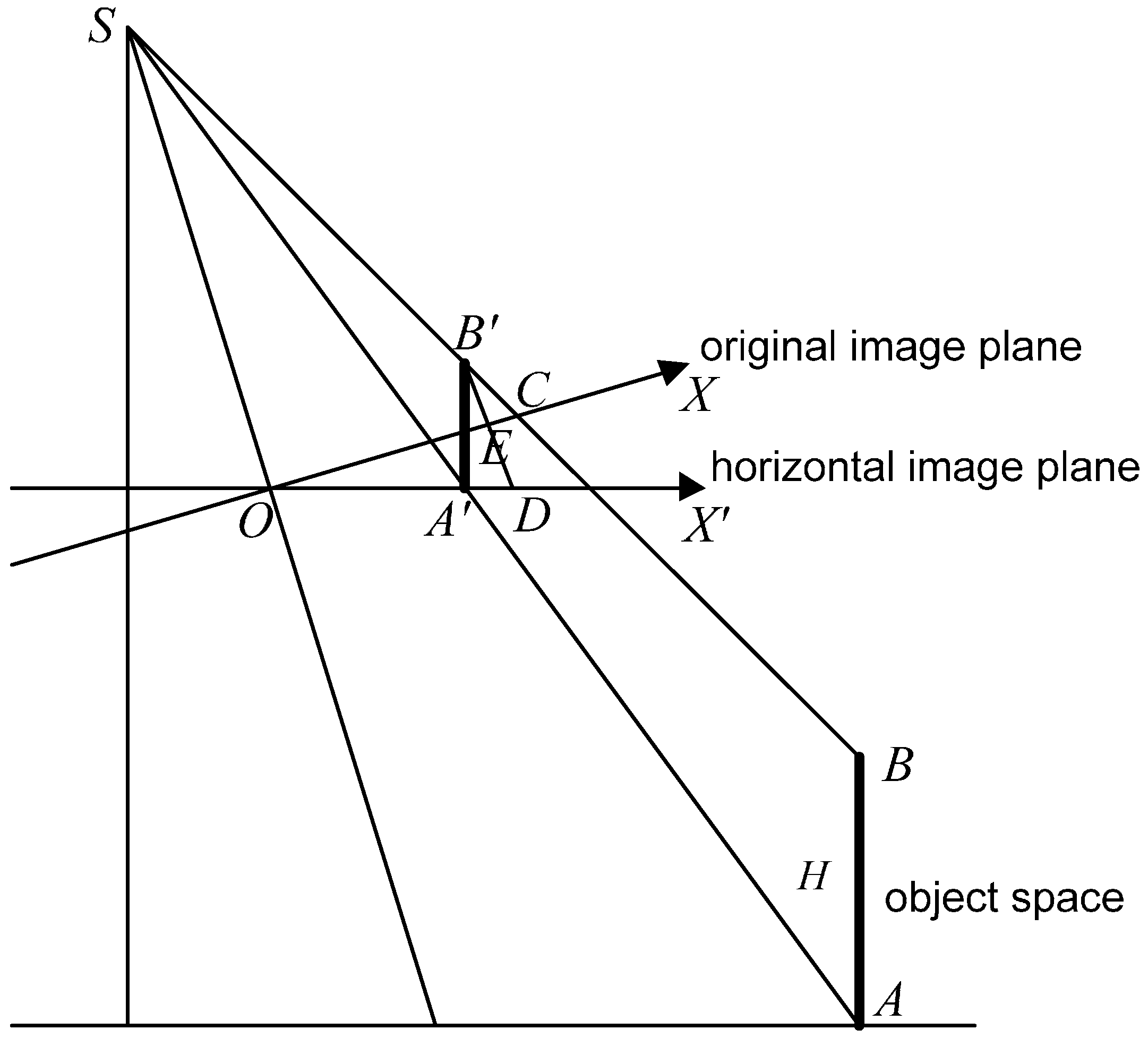
2.1. Strict Geometric Model Based on Affine Transformation
2.2. Rigorous LBTM Based on the Generalized Point Strategy
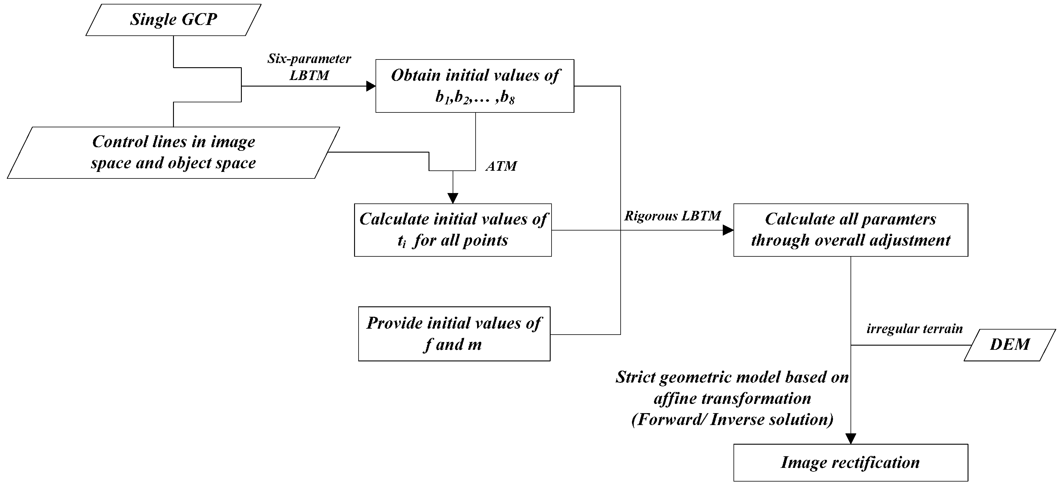
3. Image Rectification by Rigorous LBTM
3.1. Preprocessing by Six-Parameter LBTM
3.2. Overall Adjustment of Rigorous LBTM
3.3. Image Rectification by Rigorous LBTM
4. Results and Discussion
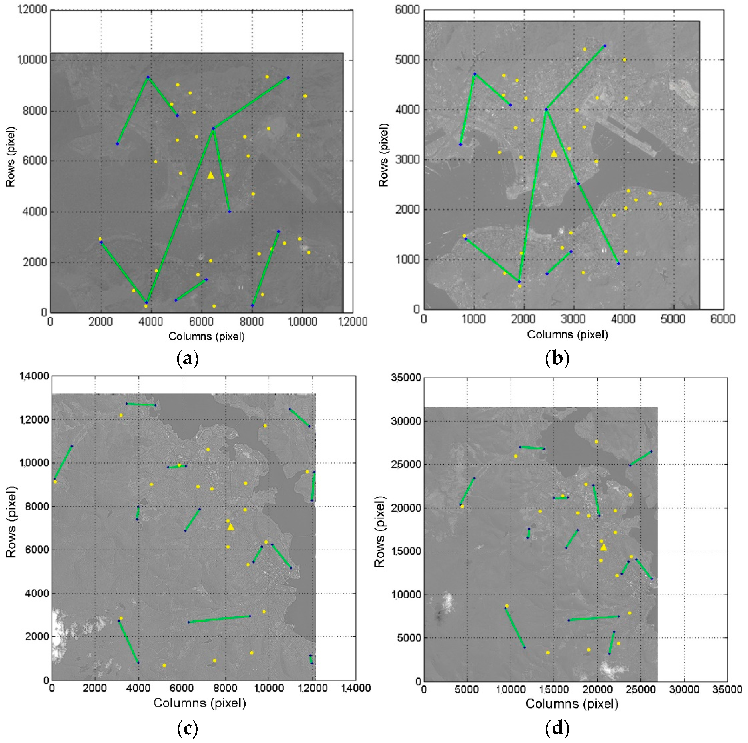
4.1. Data Source and Experiment Scheme
4.2. Performance of Rigorous LBTM to Different Datasets
4.3. Accuracy Verification of Rigorous LBTM Based on Real Control Lines
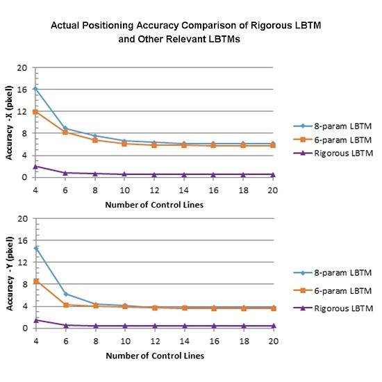
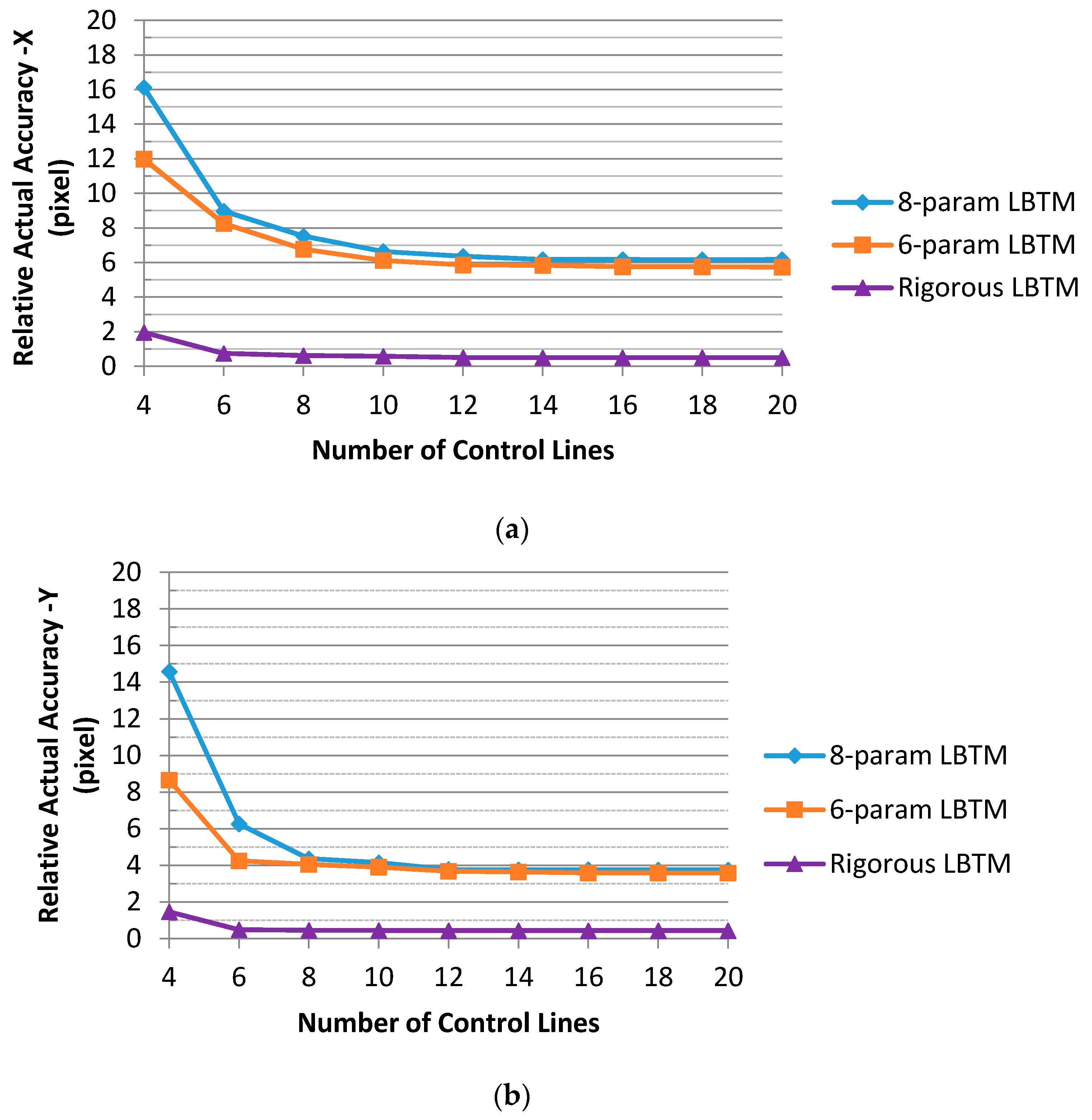
4.4. Influence of Control Lines Number to LBTMs
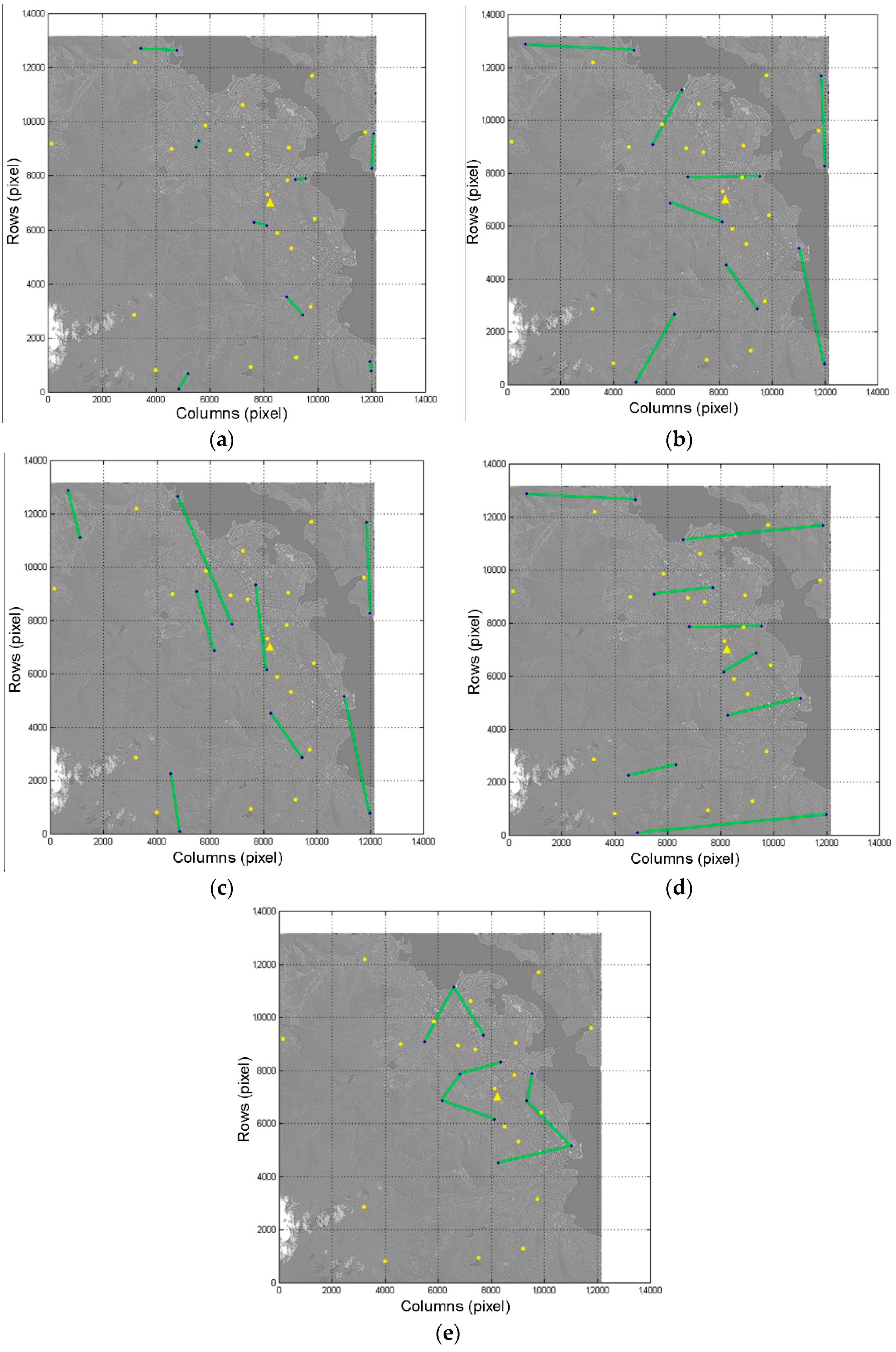
4.5. Influence of Control Lines’ Distribution on LBTMs
4.6. Discussion
5. Conclusions
Acknowledgments
Author Contributions
Conflicts of Interest
References
- Åstrand, P.J.; Bongiorni, M.; Crespi, M.; Fratarcangeli, F.; Da Costa, J.N.; Pieralice, F.; Walczynska, A. The potential of WorldView-2 for ortho-image production within the “control with remote sensing programme” of the European Commission. Int. J. Appl. Earth Obs. Geoinf. 2012, 19, 335–347. [Google Scholar] [CrossRef]
- Poli, D.; Toutin, T. Review of developments in geometric modelling for high resolution satellite pushbroom sensors. Photogramm. Rec. 2011, 27, 58–73. [Google Scholar] [CrossRef]
- Holland, D.; Boyd, D.; Marshall, P. Updating topographic mapping in great britain using imagery from high-resolution satellite sensors. ISPRS J. Photogramm. Remote Sens. 2006, 60, 212–223. [Google Scholar] [CrossRef]
- Robertson, B.C. Rigorous geometric modeling and correction of quickbird imagery. In Proceedings of the IGARSS’03, Toulouse, France, 21–25 July 2003.
- Toutin, T. Geometric processing of remote sensing images: Models, algorithms and methods. Int. J. Remote Sens. 2004, 25, 1893–1924. [Google Scholar] [CrossRef]
- Li, R.X.; Niu, X.T.; Liu, C.; Deshpande, S. Impact of imaging geometry on 3D geopositioning accuracy of stereo IKONOS imagery. Photogramm. Eng. Remote Sens. 2009, 75, 1119–1125. [Google Scholar] [CrossRef]
- Okamoto, A.; Ono, T.; Akamatsu, S.; Fraser, C.S.; Hattori, S.; Hasegawa, H. Geometric characteristics of alternative triangulation models for satellite imagery. In Proceedings of the ASPRS Annual Conference, Portland, OR, USA, 17–21 May 1999.
- El-Manadili, Y.; Novak, K. Precision rectification of SPOT imagery using the direct linear transformation model. Photogramm. Eng. Remote Sens. 1996, 62, 67–72. [Google Scholar]
- Tao, C.V.; Hu, Y. A comprehensive study of the rational function model for photogrammetric processing. Photogramm. Eng. Remote Sens. 2001, 67, 1347–1357. [Google Scholar]
- Wang, Y.N. Automated triangulation of linear scanner imagery. In Proceedings of the Joint ISPRS Workshop on Sensors and Mapping from Space, Hanover, Germany, 27–30 September 1999.
- Zhang, J.Q.; Zhang, Z.X. Strict geometric model based on affine transformation for remote sensing image with high resolution. Int. Arch. Photogramm. Remote Sens. 2002, 34, 309–312. [Google Scholar]
- Zhang, J.Q.; Zhang, Y.; Cheng, Y. Block adjustment based on new strict geometric model of satellite images with high resolution. Int. Arch. Photogramm. Remote Sens. Spat. Inf. Sci. 2004, 35, 80–84. [Google Scholar]
- Fraser, C.S.; Yamakawa, T. Insights into the affine model for high-resolution satellite sensor orientation. ISPRS J. Photogramm. Remote Sens. 2004, 58, 275–288. [Google Scholar] [CrossRef]
- Zhang, Y.J.; Lu, Y.H.; Wang, L.; Huang, X. A new approach on optimization of the rational function model of high-resolution satellite imagery. IEEE Trans. GeoSci. Remote 2012, 50, 2758–2764. [Google Scholar] [CrossRef]
- Xiong, Z.; Zhang, Y. A generic method for RPC refinement using ground control information. Photogramm. Eng. Remote Sens. 2009, 75, 1083–1092. [Google Scholar] [CrossRef]
- Hu, Y.; Tao, C.V.; Croitoru, A. Understanding the rational function model: Methods and applications. Int. Arch. Photogramm. Remote Sens. 2004, 35, 423–428. [Google Scholar]
- Tao, C.V.; Hu, Y. 3D reconstruction methods based on the rational function model. Photogramm. Eng. Remote Sens. 2002, 68, 705–714. [Google Scholar]
- Shaker, A.; Yan, W.Y.; Easa, S. Using stereo satellite imagery for topographic and transportation applications: An accuracy assessment. GISci. Remote Sens. 2010, 47, 321–337. [Google Scholar] [CrossRef]
- Tao, C.V.; Hu, Y. Updating solutions of the rational function model using additional control information. Photogramm. Eng. Remote Sens. 2002, 68, 715–724. [Google Scholar]
- Fraser, C.S.; Hanley, H.B. Bias compensation in rational functions for IKONOS satellite imagery. Photogramm. Eng. Remote Sens. 2003, 69, 53–58. [Google Scholar] [CrossRef]
- Tong, X.H.; Liu, S.J.; Weng, Q.H. Bias-corrected rational polynomial coefficients for high accuracy geo-positioning of QuickBird stereo imagery. ISPRS J. Photogramm. Remote Sens. 2010, 65, 218–226. [Google Scholar] [CrossRef]
- Habib, A.; Morgan, M.; Kim, E.M.; Cheng, R. Linear features in photogrammetric activities. Int. Arch. Photogramm. Remote Sens. 2004, 35, 610–615. [Google Scholar]
- Tommaselli, A.M.G.; Lugnani, J.B. An alternative mathematical model to the collinearity equation using straight features. Int. Arch. Photogramm. Remote Sens. 1988, 27, 765–774. [Google Scholar]
- Long, T.F.; Jiao, W.L.; He, G.J.; Zhang, Z.M.; Cheng, B.; Wang, W. A generic framework for image rectification using multiple types of feature. ISPRS J. Photogramm. Remote Sens. 2015, 102, 161–171. [Google Scholar] [CrossRef]
- Mulawa, D.C.; Mikhail, E.M. Photogrammetric treatment of linear features. Int. Arch. Photogramm. Remote Sens. 1988, 27, 383–393. [Google Scholar]
- Zhang, Y.J.; Hu, B.H.; Zhang, J.Q. Relative orientation based on multi-features. ISPRS J. Photogramm. Remote Sens. 2011, 66, 700–707. [Google Scholar] [CrossRef]
- Junior, J.M.; Tommaselli, A.M.G. Exterior orientation of CBERS-2B imagery using multi-feature control and orbital data. ISPRS J. Photogramm. Remote Sens. 2013, 79, 219–225. [Google Scholar] [CrossRef]
- Zhang, J.Q.; Zhang, H.W.; Zhang, Z.X. Exterior orientation for remote sensing image with high resolution by linear feature. Int. Arch. Photogramm. Remote Sens. 2004, 35, 76–79. [Google Scholar]
- Ok, A.O.; Wegner, J.D.; Heipke, C.; Rottensteiner, F.; Soergel, U.; Toprak, V. Matching of straight line segments from aerial stereo images of urban areas. ISPRS J. Photogramm. Remote Sens. 2012, 74, 133–152. [Google Scholar] [CrossRef]
- Dare, P.; Dowman, I. An improved model for automatic feature-based registration of SAR and SPOT images. ISPRS J. Photogramm. Remote Sens. 2001, 56, 13–28. [Google Scholar] [CrossRef]
- Habib, A.F.; Morgan, M.; Lee, Y.R. Bundle adjustment with self–calibration using straight lines. Photogramm. Rec. 2002, 17, 635–650. [Google Scholar] [CrossRef]
- Shaker, A. The line based transformation model (LBTM): A new approach to the rectification of high-resolution satellite imagery. Int. Arch. Photogramm. Remote Sens. Spat. Inf. Sci. 2004, 35, 850–856. [Google Scholar]
- Shaker, A. Point and Line Based Transformation Models for High Resolution Satellite Image Rectification. Ph.D. Thesis, The Hong Kong Polytechnic University, Kowloon, Hong Kong, China, 2004. [Google Scholar]
- Shi, W.Z.; Shaker, A. The Line-Based Transformation Model (LBTM) for image-to-image registration of high-resolution satellite image data. Int. J. Remote Sens. 2006, 27, 3001–3012. [Google Scholar] [CrossRef]
- Elaksher, A.F. Developing and implementing line-based transformation models to register satellite images. Int. Arch. Photogramm. Remote Sens. Spat. Inf. Sci. 2008, 37, 1305–1309. [Google Scholar]
- Elaksher, A.F. Potential of using automatically extracted straight lines in rectifying high-resolution satellite images. Int. J. Remote Sens. 2012, 33, 1–12. [Google Scholar] [CrossRef]
- Teo, T.A. Line-based rational function model for high-resolution satellite imagery. Int. J. Remote Sens. 2013, 34, 1355–1372. [Google Scholar] [CrossRef]
- Zhang, Z.X.; Zhang, J.Q. Generalized point photogrammetry and its application. Int. Arch. Photogramm. Remote Sens. 2005, 35, 526–530. [Google Scholar]
- Zhang, Z.X.; Zhang, Y.J.; Zhang, J.Q.; Zhang, H.W. Photogrammetric modeling of linear features with generalized point photogrammetry. Photogramm. Eng. Remote Sens. 2007, 73, 1119–1127. [Google Scholar] [CrossRef]
- Fan, H. Theory of Errors and Least Squares Adjustment; Division of Geodesy: Stockholm, Sweden, 2010. [Google Scholar]
- Mikhail, E.M.; Bethel, J.S.; McGlone, J.C. Introduction to Modern Photogrammetry; John Wiley & Sons Inc.: New York, NY, USA, 2001. [Google Scholar]


| Datasets | IKONOS_HK | ZIYUAN_HK | IKONOS_HB | GEOEYE_HB |
|---|---|---|---|---|
| Sensor Type | IKONOS (Pan) | ZiYuan-3 (Pan) | IKONOS (Pan) | GeoEye-1 (Pan) |
| Coverage Area | Hong Kong, China | Hong Kong, China | Hobart, Australia | Hobart, Australia |
| Terrain Variation | Undulated | Undulated | Hilly | Hilly |
| Elevation Range (m) | 200 | 200 | 500 | 500 |
| Coordinate System | WGS 84 UTM | WGS 84 UTM | WGS 84 UTM | WGS 84 UTM |
| GSD (m) | 1.0 | 2.1 | 1.0 | 0.5 |
| Focal Length (m) | 10.0 | 1.7 | 10.0 | 13.3 |
| Image Frame (pixel) | 11,604 × 10,280 | 4372 × 6165 | 13,148 × 12,124 | 31,668 × 26,928 |
| Pixel Size (μm) | 12.0 | 7.0 | 12.0 | 8.0 |
| Control Schemes | Datasets | Numbers in LBTMs | Numbers in PBTMs | |||
|---|---|---|---|---|---|---|
| Control Lines | Single GCP | Check Points | Control Points | Check Points | ||
| Control Scheme I | IKONOS_HK | 8 | 1 | 29 | 13 | 29 |
| Control Scheme II | ZIYUAN_HK | 8 | 1 | 29 | 12 | 29 |
| Control Scheme III | IKONOS_HB | 12 | 1 | 20 | 24 | 20 |
| Control Scheme IV | GEOEYE_HB | 12 | 1 | 20 | 24 | 20 |
| Control Schemes | Datasets | Relative Actual Accuracy | LBTMs | PBTMs | |||
|---|---|---|---|---|---|---|---|
| 8-Param LBTM | 6-Param LBTM | Rigorous LBTM | ATM | Rigorous ATM | |||
| Control Scheme I | IKONOS_HK | XRMS (pixel) | 1.4714 | 1.4485 | 0.9928 | 0.9961 | 0.9922 |
| YRMS (pixel) | 1.3009 | 1.2508 | 0.9381 | 0.9389 | 0.9351 | ||
| Control Scheme II | ZIYUAN_HK | XRMS (pixel) | 2.4784 | 2.2105 | 1.4164 | 1.3959 | 1.3901 |
| YRMS (pixel) | 1.1845 | 1.1634 | 1.3177 | 1.2101 | 1.1296 | ||
| Control Scheme III | IKONOS_HB | XRMS (pixel) | 6.3520 | 5.8500 | 0.5029 | 1.0475 | 0.4977 |
| YRMS (pixel) | 3.7699 | 3.6705 | 0.4353 | 0.4976 | 0.3660 | ||
| Control Scheme IV | GEOEYE_HB | XRMS (pixel) | 8.0303 | 7.3253 | 1.5470 | 1.7821 | 1.4574 |
| YRMS (pixel) | 5.5918 | 5.5669 | 0.8728 | 1.0073 | 0.5215 | ||
| Control Schemes | Relative Actual Accuracy | Datasets | |
|---|---|---|---|
| IKONOS_HK | ZIYUAN_HK | ||
| Control Scheme V | XRMS (pixel) | 0.9922 | 1.4162 |
| YRMS (pixel) | 0.9351 | 1.3168 | |
| Control Scheme VI | XRMS (pixel) | 0.9923 | 1.4165 |
| YRMS (pixel) | 0.9380 | 1.3172 | |
| Control Schemes | Relative Actual Accuracy | LBTMs | ||
|---|---|---|---|---|
| 8-Param LBTM | 6-Param LBTM | Rigorous LBTM | ||
| Control Scheme VII | XRMS (pixel) | 6.5383 | 6.0626 | 0.5600 |
| YRMS (pixel) | 4.1577 | 3.6783 | 0.4434 | |
| Control Scheme VIII | XRMS (pixel) | 15.1325 | 10.3079 | 0.8513 |
| YRMS (pixel) | 7.6346 | 5.9687 | 0.4843 | |
| Control Scheme IX | XRMS (pixel) | 8.3384 | 7.5454 | 0.6724 |
| YRMS (pixel) | 7.2757 | 5.4367 | 0.4823 | |
| Control Scheme X | XRMS (pixel) | 12.7432 | 9.7182 | 0.8262 |
| YRMS (pixel) | 4.9636 | 4.2063 | 0.4595 | |
| Control Scheme XI | XRMS (pixel) | 15.6346 | 11.6248 | 1.0497 |
| YRMS (pixel) | 9.7341 | 7.0535 | 0.6671 | |
© 2016 by the authors; licensee MDPI, Basel, Switzerland. This article is an open access article distributed under the terms and conditions of the Creative Commons Attribution (CC-BY) license (http://creativecommons.org/licenses/by/4.0/).
Share and Cite
Hu, K.; Shi, W. Rigorous Line-Based Transformation Model Using the Generalized Point Strategy for the Rectification of High Resolution Satellite Imagery. Remote Sens. 2016, 8, 743. https://doi.org/10.3390/rs8090743
Hu K, Shi W. Rigorous Line-Based Transformation Model Using the Generalized Point Strategy for the Rectification of High Resolution Satellite Imagery. Remote Sensing. 2016; 8(9):743. https://doi.org/10.3390/rs8090743
Chicago/Turabian StyleHu, Kun, and Wenzhong Shi. 2016. "Rigorous Line-Based Transformation Model Using the Generalized Point Strategy for the Rectification of High Resolution Satellite Imagery" Remote Sensing 8, no. 9: 743. https://doi.org/10.3390/rs8090743
APA StyleHu, K., & Shi, W. (2016). Rigorous Line-Based Transformation Model Using the Generalized Point Strategy for the Rectification of High Resolution Satellite Imagery. Remote Sensing, 8(9), 743. https://doi.org/10.3390/rs8090743