Article

Monitoring Agronomic Parameters of Winter Wheat Crops with Low-Cost UAV Imagery

1
Leibniz Institute for Agricultural Engineering, Potsdam-Bornim e.V., Max-Eyth-Allee 100, 14469 Potsdam, Germany
2
Julius Kühn-Institut, Federal Research Centre for Cultivated Plants, Institute for Plant Protection in Field Crops and Grassland, Messeweg 11-12, 38104 Braunschweig, Germany
3
Geography Department, Humboldt University Berlin, Rudower Chaussee 16, Unter den Linden 6, 10099 Berlin, Germany
*
Author to whom correspondence should be addressed.
Remote Sens. 2016, 8(9), 706; https://doi.org/10.3390/rs8090706
Submission received: 6 May 2016 / Revised: 17 August 2016 / Accepted: 24 August 2016 / Published: 27 August 2016
(This article belongs to the Special Issue Remote Sensing in Precision Agriculture)

Abstract

:
Monitoring the dynamics in wheat crops requires near-term observations with high spatial resolution due to the complex factors influencing wheat growth variability. We studied the prospects for monitoring the biophysical parameters and nitrogen status in wheat crops with low-cost imagery acquired from unmanned aerial vehicles (UAV) over an 11 ha field. Flight missions were conducted at approximately 50 m in altitude with a commercial copter and camera system—three missions were performed between booting and maturing of the wheat plants and one mission after tillage. Ultra-high resolution orthoimages of 1.2 cm·px−1 and surface models were generated for each mission from the standard red, green and blue (RGB) aerial images. The image variables were extracted from image tone and surface models, e.g., RGB ratios, crop coverage and plant height. During each mission, 20 plots within the wheat canopy with 1 × 1 m2 sample support were selected in the field, and the leaf area index, plant height, fresh and dry biomass and nitrogen concentrations were measured. From the generated UAV imagery, we were able to follow the changes in early senescence at the individual plant level in the wheat crops. Changes in the pattern of the wheat canopy varied drastically from one mission to the next, which supported the need for instantaneous observations, as delivered by UAV imagery. The correlations between the biophysical parameters and image variables were highly significant during each mission, and the regression models calculated with the principal components of the image variables yielded R2 values between 0.70 and 0.97. In contrast, the models of the nitrogen concentrations yielded low R2 values with the best model obtained at flowering (R2 = 0.65). The nitrogen nutrition index was calculated with an accuracy of 0.10 to 0.11 NNI for each mission. For all models, information about the surface models and image tone was important. We conclude that low-cost RGB UAV imagery will strongly aid farmers in observing biophysical characteristics, but it is limited for observing the nitrogen status within wheat crops.

Graphical Abstract

1. Introduction

Recently, unmanned aerial vehicles (UAVs) have been introduced into agricultural research to monitoring crops [1]. In contrast to satellite imagery and aircraft-based remote sensing, UAVs can be used frequently during the entire growth period. The main benefits are simple mission planning, instantaneous operation with low man power and imaging below cloud cover [2]. By carrying low-cost commercial camera systems, UAVs provide ultra-high resolution images of the crop canopy due to the low flight altitude. Current developments in photogrammetric algorithms are specifically adapted to the needs of UAV imagery. Thousands of images can be nearly automatically processed via ready-to-use software to produce orthoimages or surface models. Because wheat is the crop grown with the highest acreage [3] there is a strong interest in obtaining spatial and temporal information about the wheat canopy in high resolution, e.g., to adapt nitrogen and pesticide application site-specifically to improve production efficiency [4,5,6].
The periodic monitoring of the canopy biophysical parameters, such as biomass, leaf area index (LAI) and plant height (PHT), is essential to understanding crop development, variations in canopy reflectance and net ecosystem exchange or nitrogen and pesticide demand during the growth season [7,8,9]. These parameters and derivatives are important for precision agriculture, remote sensing, crop modeling, ecosystem modeling and climate modeling. Crop growth models use a wide range of biophysical parameters to estimate future yield as input and validation [10,11]. Biophysical parameters may further deliver vital information about the specific infection situation with fungal diseases to make field-specific decisions on plant protection [12]. The availability of this information at the field scale would enable a new generation of decision support systems that can optimize fungicide application in winter wheat, e.g., the prototype “proPlant expert” precisely recommends maximum application rates for up to three management zones within a field according to the yield expectation [7].
The monitoring of nitrogen (N) is an essential tool for investigating many metabolic and structural processes in maturing wheat plants, such as yield formation and health status. Because N is not immobilized in soils and an abundant reservoir of plant-available N is not present, it is important for optimal crop production to supply N by applying fertilizer throughout plant growth. However, excessive use of fertilizer eventually leads to unwanted N-leaching into groundwater or N-contamination of surface run-off water, contributing to environmental pollution, which is to be avoided [13]. The N status cannot be estimated from the leaf nitrogen content alone but biophysical parameters of the wheat canopy should also be taken into account. For example, the nitrogen nutrition index (NNI), i.e., the ratio between the actual N concentration (Nt) observed in the plants and the critical N concentration related to dry biomass (Nct), has been used to reliably characterize the N status of wheat crops during the vegetative period [14]. NNI values >1 indicate excessive N supply (over-fertilization), whereas suboptimal N supply is indicated by values <1. Especially during flowering and the grain-filling growth stage, NNI is a good indicator of N deficiency affecting grain yield and grain protein [14,15].
Due to the complex interrelationship between many environmental factors, such as soil heterogeneity, cultivation and land surface, the parameters described above show high spatial and temporal variability so that a high measurement density would be needed to reflect their spatial patterns within the field [16]. It has been shown that site-specific management strategies in the context of precision farming increase management efficiency [4]. However, accurate measurements of these parameters are time consuming or destructive. For example, the calculation of the NNI involves the cutting of fresh biomass, subsequent drying and the determination of Nt using the Dumas or Kjeldahl method in the laboratory [17].
To become more efficient, indirect methods using sensors for estimating those parameters have been proposed and implemented. At the plot scale, sensor principles are available that enable on-spot measurements without destructing the canopy, mostly with direct contact to wheat plants. For example, leaf chlorophyll meters relate the light transmittance or fluorescence on leaf parts to chlorophyll content and, by using certain indices, to leaf Nt [18]. The LAI can be modeled by devices measuring sunlight interception in the wheat canopy using radiative transfer models [19]. Most of these principles involve time-demanding measurements or sophisticated measurement protocols that can only be performed manually in a stop-and-go mode. Their use for online or high-throughput measurements was discussed only very recently in research, e.g., mobile LAI determination by sunlight interception [20].
For the real-time determination of biophysical parameters and N status, many active sensing approaches have been studied, such as LiDAR, optical sensors and ultra-sound sensors [21,22,23,24], in addition to more refined solutions, e.g., the pendulum operating measurement principle Crop-Meter [25,26]. These sensors are mainly installed within or up to two meters above the canopy and are bound to a ground-driven vehicle such as a tractor. They have the advantage that they deliver information about the wheat canopy immediately and in high resolution. Optical sensors mostly use specific spectral vegetation indices (SVI) in the visual and infrared part of the spectrum. The GreenSeeker® (Trimble, Sunnyvale, CA, USA) detect the reflection between 656 nm (VIS) and 774 nm (NIR), whereas the CropCircle® (Holland Scientific Inc., Lincoln, NE, USA) allows for more freedom in the choice of wavelengths by using different filters [23]. To map larger areas, spectral vegetation indices (SVI) from satellite-based and aircraft-based remote sensing imagery have been related to those parameters [27,28]. In contrast to proximal sensing, these data have lower spatial and temporal resolution. UAV imagery might be able to close the gap between the plot scale, covered by manual sensors and proximal sensors, and the regional scale, covered by traditional remote sensing, because of their high spatial resolution and almost instantaneous availability for practitioners and experts in agriculture. Most studies have investigated the relationship between biophysical parameters and UAV imagery, e.g., biomass [29,30,31,32,33], LAI [34,35,36,37,38], plant height [30] and grain yield [39], whereas fewer studies have shown the relationship between nitrogen and UAV imagery [31,35,40,41] in wheat crops, so far. We summarized existing research studies relating UAV imagery with some agronomic parameters of wheat crops in Table S1. Only Pölönen, et al. [31] investigated dry biomass and total nitrogen content in combination with UAV hyperspectral imagery, which allowed them to calculate the under or over nourishment of the wheat plants during crop growth using the NNI. To the best of our knowledge, low cost UAV imagery has not been tried for estimating NNI in cereal crops. Moreover, many studies examined only fields or parts of fields with sizes smaller than 3 ha.
The objective of our work was therefore to study the prospects of low cost UAV imagery for monitoring biophysical plant parameters, N-content and NNI of wheat crops from a more practical viewpoint closer to agricultural routines. Three UAV missions were carried out between booting and maturity over an 11 ha field under soil-induced water deficit conditions and we acquired a large set of aerial images with a consumer level camera. Based on that, ultra-high resoluted orthoimages and surface models were computed through photogrammetric processing. We demonstrated the applicability of UAV imagery for recognizing the spatio-temporal patterns of the wheat canopy development, as observed in this field. Furthermore, we investigated the relationship of biophysical parameters, i.e., plant height, LAI and biomass, as well as, nitrogen status, with the image variables that were derived from the UAV imagery at specific dates. Regarding this relationship, we determined its strength to model the spatial variability of those parameters with linear regression in order to fulfil precision agricultural needs. This is important in order to establish a monitoring system for crop variability that allows fast production of maps for end users such as farmers or agricultural services adopting precision agriculture. This may improve typical applications of precision agriculture such as variable rate fertilization or precision plant protection.

2. Materials and Methods
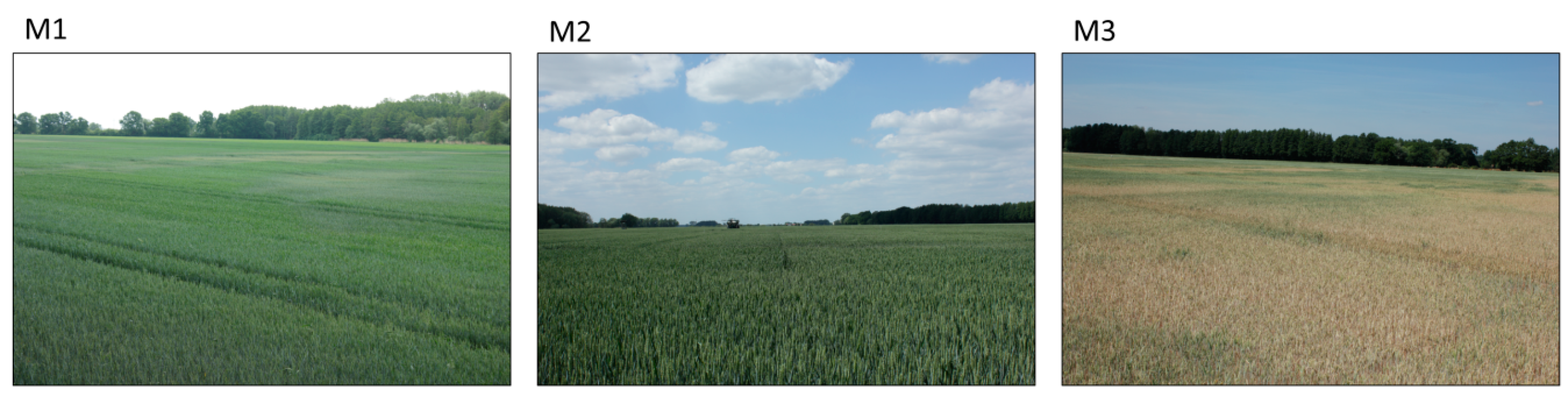
2.1. Test Site

The study was conducted within a field in Eastern Germany during the spring season in 2015 (51°49′N, 12°42′E). The soil development in the field was influenced by recent flood plain deposits of the Elbe River. The main soil type is a fluvic cambisol and the soil texture varies between sand, loamy sand and sandy loam. The crop grown was winter wheat (Triticum aestivum L. var. ‘Linus’). The seed row distance was 0.12 m, and the average crop density was between 440 and 480 ears·m−2.

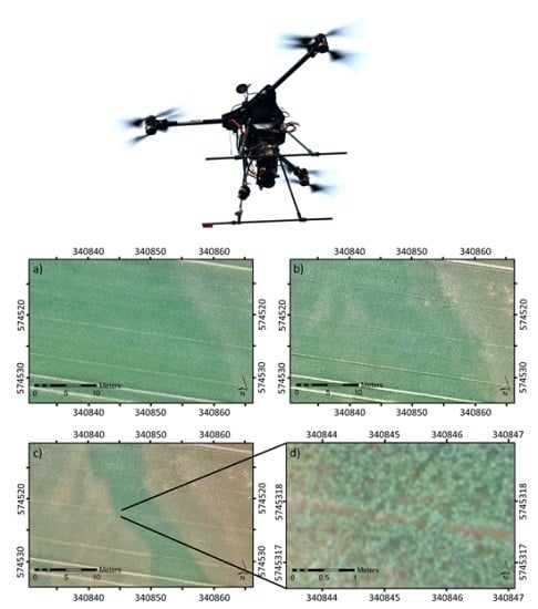
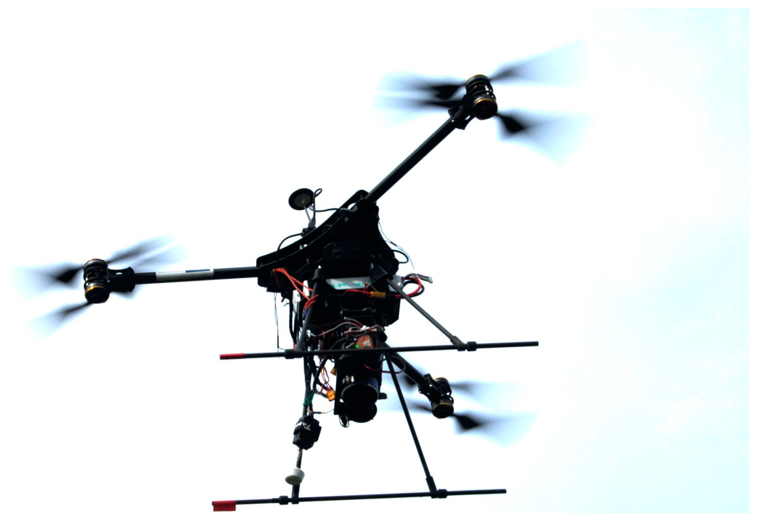
2.2. UAV System and Flight Missions

We used a hexacopter (P-Y6, Hexapilots, Dresden, Germany) to carry a commercial camera system to acquire the aerial images for this study (Figure 1). The hexacopter consisted of six propellers aligned in a three arm mounting with two propellers attached to each arm using the push/pull principle for failure safety. The navigation control system was a DJI Wookong M (DJI Innovations, Shenzhen, China) with an integrated GNSS receiver, which enabled user-defined waypoint tracking. Power supply was ensured with lithium polymer batteries (10,000 mAh/5 s). With this setup, including the camera, approximately 15 min flight duration was achieved.
For image acquisition, we used a Sony Nex 7 point and shoot camera with the following specifications: 24 megapixels, 23.5 × 15.4 mm sensor and E16 mm F2.8 fixed lens (Sony Corporation, Tokyo, Japan). The camera was mounted onto a gimbal underneath the copter. The DJI software triggered image capturing, and the position of the copter was recorded by a GPS device.
The flight missions were planned to cover approximately 13 ha of ground area. The orthoimages and surface models were later clipped to 11 ha to correspond to the study area. Parallel tracks were flown with a between-track distance of 11 m at an altitude of 50 m which is a side-lap of 60%. The frequency of image capture was set to correspond to 60% image overlap. All images were taken from near nadir position with a ground resolution of approximately 0.012 m·px−1.

2.3. Ground Truthing

Three flight missions (M1-3) were conducted over the wheat canopy during crop growth from booting of the wheat plants until mature growth stages. An additional flight mission (M4) was performed after tillage to yield a UAV image of the ground surface. Mission dates, weather conditions and objectives of the flight missions are enlisted in Table 1.
For each mission, 20 locations were chosen with respect to the wheat variability observed at that date. These locations were selected along the tractor lanes by eye. Locations were at least 2 m distance from the tractor lane in order to be non-influenced by the clearing. At each plot, the ground area spanned by 1 × 1 m² was taken as the sample size. For georeferencing the UAV images, 20 panels were laid out along a regular grid over the field within the tractor lanes with good visibility from above before the flight missions. Panels and plots were located using the differential GPS HiPer Pro system (Topcon Positioning Systems, Inc., Livermore, CA, USA) having a relative horizontal and vertical accuracy of 3 mm and 5 mm.
At each plot, the plant height (PHT), LAI, fresh biomass (FBM), dry biomass (DBM) and Nt were determined as agronomic reference measurements. The descriptive statistics and the abbreviations used in this paper are summarized in Table 2. Wheat plants were classified according to the BBCH growth stages code of Lancashire et al. [42]. Measurements of PHT were integrated by the measured heights of the wheat plants using a folding yardstick at 10 random locations within the plot. LAI was measured using the SunScan Canopy Analysis System type SS1 (Delta-T Devices, Cambridge, UK). The LAI probe was positioned at 45° to the direction of the seed rows under the canopy, and the reference sensor was in immediate proximity above the canopy without disturbing the incoming sunlight. The LAI measurement was taken as an average of 10 individual measurements with the probe repositioned each time within the plot. All wheat plants within the plot area were then cut directly above the ground using a short reaping hook. FBM was determined immediately after cutting. DBM was measured by drying biomass samples at 60 °C for 48 h in a compartment drier. The dry plant material was milled and analyzed for Nt following the dry combustion method of Dumas [43] using an elemental analyzer (Vario MAX CN Elemental Analyser, Elementar, Hanau, Germany).

2.4. Image Pre-Processing

All aerial images were recorded in RAW data format and lossless converted to the tagged image file format (TIFF) in standard RGB color space. The full camera calibration matrix, including non-linear distortion coefficients, was estimated for the camera sensor using the Agisoft Lens software (v. 0.4.2, Agisoft LLC, St. Petersburg, Russia) by repetitively taking photographs of a checkerboard pattern. The Agisoft Lens software uses a pinhole camera model for lens calibration, and the distortion correction is modeled by Brown’s distortion model. We used a number of radiometric pre-processing steps to improve the final UAV image mosaicking and the surface model generation results, as shown below. These algorithms were programmed in Matlab 2015b. To reduce colorimetric alterations, the following corrections were conducted only on the value channel of the HSV transformed aerial images. The corrected HSV images were then transformed back to RGB space.
To diminish the effect of brightness reduction from the image center to the borders due to the sensor optics, all images were empirically corrected using the vignette correction algorithm proposed by Zheng et al. [44]. This processing involved calculating a mean image from a selection of homogeneous aerial images (n = 80). In our case, images were selected that depicted only the wheat canopy without prominent features such as trees. The further pre-processing steps were performed on the vignette-corrected images.
For better photogrammetric processing, contrast-enhanced images were produced from each aerial image. This was achieved by contrast limited adaptive histogram equalization (CLAHE). Each image was divided into eight tiles. Within each tile, the contrast was enhanced by histogram equalization following the Gaussian distribution. To avoid artificial boundaries, the neighboring tiles were then joined using bilinear interpolation. The images corrected by CLAHE were used during the mosaicking process and surface model generation.
Different incidence and viewing angles may result in unwanted radiometric variations in the aerial images related to the bidirectional reflectance distribution function (BRDF). This effect was reduced following the empirical BRDF correction algorithm suggested by Lelong et al. [35]. In short, each image was block-wise averaged to a smaller representation of the image by bilinear interpolation, then smoothed by Gaussian filtering and finally over-sampled onto the original image with bi-cubic interpolation. Then, the inverted, smoothed values were subtracted from the original values. Specifically, all images were subdivided into 400 × 400 pixel blocks, and the Gaussian filter size used was a 3 × 3 pixel window. The BRDF set of images was used for the final texturing of the orthoimage.

2.5. Photogrammetric Processing

The vignette-corrected and CLAHE pre-processed images were used in the semi-automated processing flow of the photogrammetry software Agisoft PhotoScan (v. 1.2.4, Agisoft LLC, St. Petersburg, Russia) to generate orthoimages and surface models for M1-4. The software implements Structure from Motion to estimate a 3D point cloud from the overlapping aerial images [45]. Using feature detection and description algorithms, key points between overlapping images that bear geometrical similarities in their immediate surroundings were selected. In the first step, a sparse 3D point cloud was generated to align the images and estimate the exact camera positions. We used the options ‘high’ and ‘generic’. In the second step, a dense, multi-view stereo reconstruction on the aligned image set operating on the pixel level was applied that generated a dense 3D point cloud. For this, we used the options ‘medium’ and ‘mild’ depth filtering. We used this setting because higher quality takes exponentially more time and demands more computational resources. Prior tests with the software showed “medium” as a good compromise with adequate processing time (4.6 cm/pix resolution error). The mesh was generated using the option ‘height field’ to produce the orthoimages and the surface models. To texture the orthoimages, the CLAHE pre-processed images were exchanged with the BRDF-corrected images. The texturing was performed with the software-implemented color correction. The ground resolution of the orthoimages was 0.025 m·px−1.

2.6. Extraction of Image Variables

We calculated a set of image variables from the orthoimages and the surface models at each measurement plot to relate them to the agronomic reference measurements. The image variables were computed from averaging the pixels within the plot areas. Furthermore, crop pixels were identified to calculate crop coverage (CVR). This was achieved by first converting the respective orthoimages into the LAB color space because we found the best discrimination between soil and vegetation in the a-vector corresponding to the red-green variation of the images. Secondly, within the whole orthoimage, we randomly selected regions of interest (ROI) containing only soil-related pixels. These ROIs were combined into a simple vector and the value given at the 90% percentile was used as a threshold value to differentiate between soil and vegetation pixels in the measurement plots. CVR was computed as the percentage of all vegetation pixels identified within a plot. All image variables are described in Table 3.

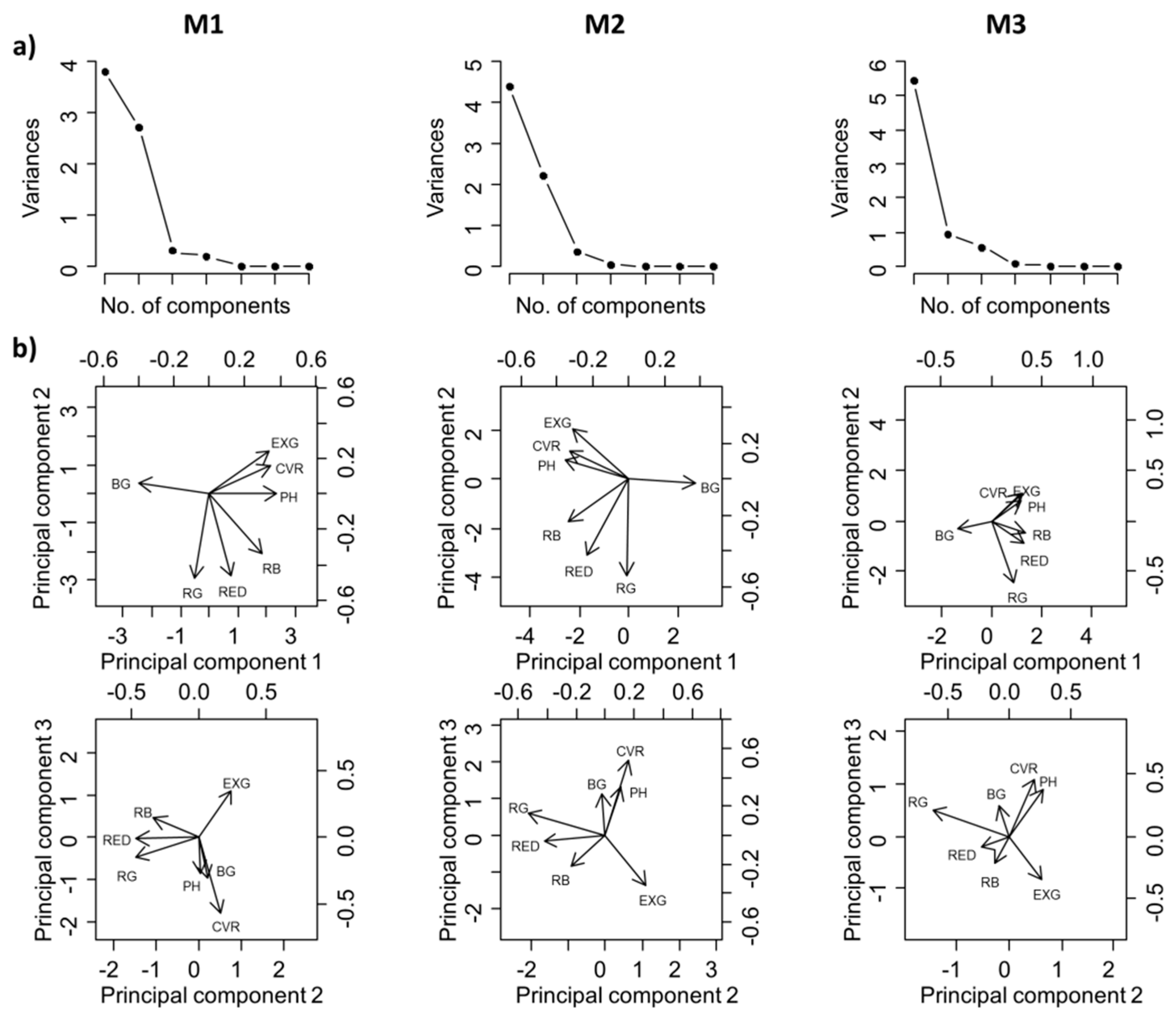
2.7. Statistical Analysis

The relationships between the image variables and reference measurements were investigated and tested for significant correlation using a Pearson correlation matrix for M1-3. Principal component analysis (PCA) was conducted to explore the structural variation and dimensionality within all image variables for M1-3. PCA was calculated using the correlation matrix to eliminate the influence of different standard deviations among the image variables. Loading plots were used to summarize the interrelationship between the image variables. Linear regression analysis was conducted using the agronomic reference measurements as dependent variables. As independent variables, the scores from the principal components (PC) that contributed sufficiently to the overall variance of the image variables were used to prevent multi-collinearity in the regression models. The best models were chosen by backward selection. Variables with p > 0.1 were deleted from the set of independent variables [46]. For model comparison, we reported the adjusted R2 values according to Wherry [47].
The NNI was calculated using the approach of Lemaire and Salette [48]:
N c t   =   a   D B M b ,
N N I   =   N t N c t
where Nct is the critical N concentration related to a specific dry biomass (DBM). Justes et al. [15] specified the dilution curve for Nct statistically on wheat crops by proposing values for a = 5.35 and b = 0.442, which were used for the NNI determination in this study.
All models were validated using an independent model and validation data set by splitting the field equally in two halves orthogonal to the tractor lane direction. As validation criteria, the R2 of validation (R2val) expressed as the squared Pearson correlation coefficient, the root mean squared error (RMSE) and the mean error (ME) were calculated:
R 2 v a l = c o v ( x , y ) v a r ( x ) v a r ( y ) ,
R M S E = i = 1 n x i y i n ,
M E = x ¯ y ¯ ,
where x and y denotes the reference and predicted values and x ¯ and y ¯ , the means of the reference and predicted values at the validation locations, n the number of validation points and cov and var the covariance and variance, respectively.

3. Results and Discussion

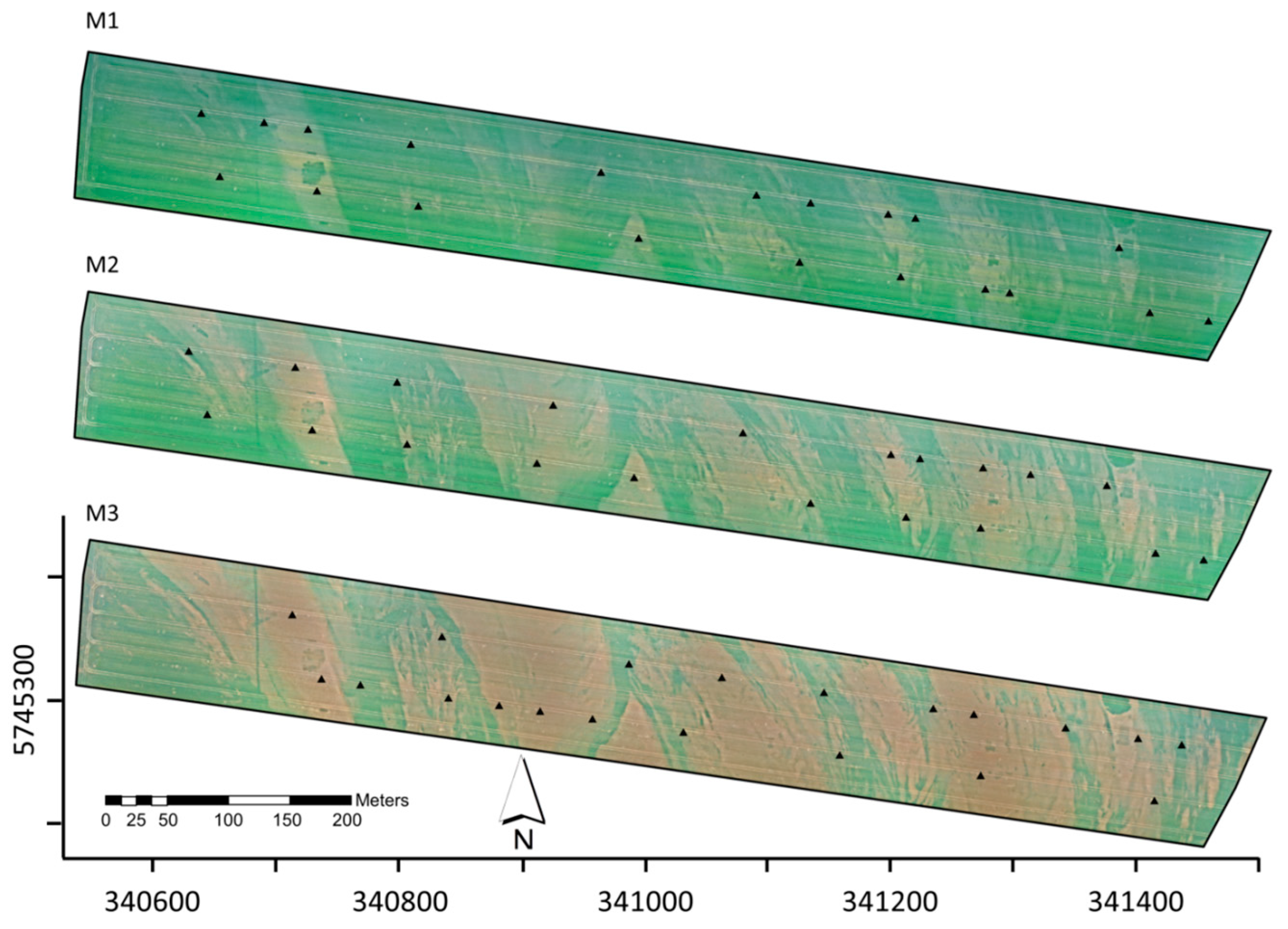
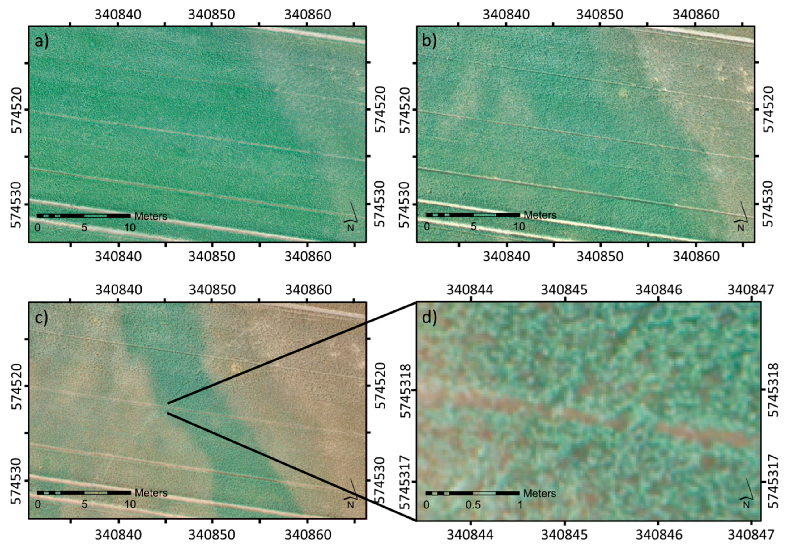
3.1. Qualitative Assessment of the Acquired UAV Imagery

Three UAV missions were flown during the growing season on 5/18/15 (M1), 6/4/15 (M2) and 6/16/15 (M3). The phenological stages of the wheat plants ranged from booting with flag leaf sheath extending (M1) to flowering (M2) to maturity (M3) (Figure 2). At the specific dates, the growth stages varied to some extent spatially across the fields due to soil heterogeneity. Generally, at locations with coarser soil texture, where water availability was lower, the growth stages tended to be more mature, whereas plant biomass was underdeveloped. This differentiation gradually increased at later dates. Plant diseases were not detected throughout all mission dates.
The distribution of the RGB colors in the orthoimages was structured according to the spatial variation of the plant coverage, growth stage, leaf vitality and degree of senescence (Figure 3). Darker greenish colors indicate areas with denser crop canopy and higher plant vitality, whereas lighter yellow-brownish colors are associated with sparser crop canopy and lower vitality. Soil-induced water deficit stress reduced leaf area development and plant height, causing spatial variation in the crop canopy throughout the field. It also invoked an earlier senescence of the leaves [49]. For M1, the lighter-colored areas corresponded to average plant water content: 64%, LAI: 2.27 and dry biomass: 0.80 kg·m−2, whereas within the greenish areas, the same parameters were higher, with plant water content: 74%, LAI: 3.61 and dry biomass: 0.92 kg·m−2. The effect of the soil-induced water deficit stress increased from M1 to M3, leading to stronger structuring in the orthoimages with an advancing image tone to more yellow and brown colors. This structuring and pattern indicates near-surface sedimentological changes. They were established by the remnants of the former fluvial geomorphology in the Pleistocene shaped by the floodplain of the river Elbe. At that time, differences in the river flow rates caused a braided river system with lots of small river channels broken by temporary islands. This resulted in highly local differences in soil texture, which is typical for the fields in this area and invoked the patterning of the wheat canopy. As observed from the zoomed representations depicted in Figure 4a–c, the wheat canopy completely changed within only a few days from M2 to M3. That change cannot be observed from M1 and can only be vaguely outlined at M2. This sudden change emphasizes the need of high temporal availability of aerial image data for cultivated land—an advantage of UAV imagery over remote sensing imagery by satellite and airplanes due to its independence of cloud conditions, its easy mission planning and low costs. Moreover, the high spatial resolution of the UAV images allows the differentiation of these changes down to the individual plant level (Figure 4d). Using these images in a geographical information system, farmers would be able to locate and monitor changes in their crops with high accuracy over the entire field. Depending on the aim of the qualitative assessment of the farmer this zoom level may become useful, e.g., plant diseases (yellow rusts) spread from small nests.
The same strong patterning as in the UAV imagery occurred in the surface models (M1-3) of the wheat canopy. As observed in Figure S1, the patterning of M1 was not the same as the ground surface model (M4). Thus, changes in the surface model of M1 may show differences in plant growth.

3.2. Relationship between Agronomic Parameters and Image Variables

The biophysical parameters FBM, DBM, LAI and PHT were highly correlated with each other at M1-3 (Table 4). Specifically, the correlation between LAI and FBM was high because plant water is mainly stored in plant leaves, and plant water varied significantly in this field.
The correlations between the biophysical parameters and the image variables were significant in most cases. Overall, the average correlation strength between all image variables and the biophysical parameters increased from M1 to M3 (r = 0.64 < 0.73 < 0.82). This increase can be explained by the higher variation and by the better differentiation of the image tone that was observed at the later missions in the field. The image variables BG and RB were the most strongly correlated. Moreover, PHTUAV, calculated from the surface models, had a valuable contribution to explaining the biophysical parameters of the wheat canopy. From M1 to M3, the correlation of PHTUAV with FBM, DBM, LAI and PHT was highly significant (r > 0.80). The only exception occurred at M1, in which PHTUAV was somewhat more weakly correlated with DBM (r = 0.68). The weaker correlation can be explained by dry matter being mainly stored in the wheat leaves and not in the wheat stems at booting stage. The dry matter in the leaves does not significantly contribute to the actual plant height [50]. This result can also be anticipated from the lower correlation of PHT with DBM at M1 compared to M2 and M3.
In contrast, Nt was only weakly or not significantly correlated with the biophysical parameters throughout all missions. We expected a significant correlation between RED and Nt because a cross-correlation between the chlorophyll content in plant leaves and the nitrogen content exists. Because chlorophyll absorbs light in the red wavelengths, it may cause variation in the RED image variable or red-related SVIs, which could be related to Nt [51,52]. The correlation of Nt with the image variables was generally higher than correlation with the biophysical parameters but it was still relatively weak. On M1 and M2, significant correlations between RED and Nt were found. However, at M3, no significant correlation existed, which can be explained by the large appearance of senescent plant leaves with no or little chlorophyll content left. The linear relationship between the chlorophyll content and Nt breaks down when the vegetation becomes senescent [28]. As the wheat reaches maturity, wheat leaves lose chlorophyll and N is used for grain development [14]. The best relationship between the chlorophyll content and Nt was found near the flowering growth state for wheat [14,18]. RED and RG had the highest correlation with Nt at M2, whereas, at M3, the biophysically related image variables PHTUAV and CVR were negatively correlated with Nt and RED was not correlated.
In Figure 5, the scree plots and the loading plots for the first few components were computed by PCA using the correlation matrix of the image variables for each of the missions as extracted at the measurement plots. The scree plots show the component variances against the components and the loading plots show the degree of the relationship to a specific PC. Loading vectors that point in the same or opposite direction indicate positively or negatively correlated variables whereas orthogonal loading vectors highlight dissimilar variables.
Most of the variance explained by the image variables was projected onto the first three principal components of the PCA as observed from the eigenvalues depicted in the scree plot (Figure 5). The loading plots show a specific multivariate grouping of the image variables. Two main groups can be identified: the image variables influenced by the red signal (RED, RG, RB) and the image variables related to the blue signal and biophysical parameters (BG, EXG, CVR, PHTUAV). On M1 and M2, the first group was mainly related to PC 2 whereas the biophysical group was related to PC 1 and PC 3. At M3, the groups became similar.

3.3. Modeling the Biophysical Wheat Parameters

We performed linear regression on PC 1-3 as independent variables. The relevant PCs were chosen by backward selection with p < 0.1 (Table 5). All models were significant at p < 0.001. The best overall model fits were obtained at the later missions (M2 and M3) for FBM and PHT (R2 > 0.92), and the lowest model fit was achieved by DBM at M1 (R2 = 0.70). Thus, model quality increased towards the later dates. This gradient was most evident for DBM, due to the reduction of plant water within the wheat canopy caused by senescence of the plant leaves. The image tone increasingly represented the variation of dry biomass in the orthoimages of the later missions. Additionally, the contribution of PC 3 is more important at M2 and M3 because the plant height has a larger influence on DBM at flowering and maturity than at booting. Overall, the contribution of the PCs varied between the models, and in almost all cases, more than one PC was significant, which emphasizes the need to use different image variables to estimate the biophysical parameters. For all models, PC 1 was a highly significant predictor. Since CVR, PHTUAV and BG load highest on PC 1, it shows that these variables are relevant for determining the biophysical parameters from UAV RGB imagery. However, the red-related image tone variables, i.e., RED, RG and RB, which loaded strongly on PC 2, had an influence on most models. Interestingly, the influence of PC 2 was relatively high for determining PHT, which means that the image tone may also support the estimation of plant height derived from the UAV crop surface models. Moreover, the inclusion of plant height information helps to linearize the other biophysical parameters in wheat crops when observed over several growth stages [53]. Therefore, it is advisable to use both the image tone and the surface models to estimate the biophysical parameters due to their strong interrelationship within the wheat canopy.

3.4. Modeling the Nitrogen Status

The models for Nt were weaker than the models for the biophysical parameters (Table 6). The importance of PC 2 specifically at M1 and M2 was related to the influence of the red-related image tone variables because of their dependence on the chlorophyll content. A highly significant model was only obtained for M2 (p < 0.001) during flowering due to the well-established physical relationship between the chlorophyll content and Nt that can be observed during this growth stage. However, PC 3 also had a significant influence at M2 and M3 because of the increasing influence of PHTUAV and the declining influence of the red image tone variables for determining Nt as was shown earlier in the correlation matrix.
To calculate the NNI, we combined the DBM and Nt estimations using Equations (1) and (2). The validation results are given in Table 7. For each mission, we obtained the same error of 0.11 NNI. The NNI reference values indicated a slight undernourishment of the wheat crops, with most NNI values smaller than 1.0, and the variability of the NNI was relatively small for the heterogeneous field (Figure S3). The scatter plots showed a linear relationship between validations and predictions but were influenced by some extremely erroneous predictions, specifically at M3.

4. Discussion

Compared to studies investigating proximal sensing to estimate biophysical crop parameters, the UAV image variables were competitive. Several studies tested LiDAR systems from a tractor as an online proximal sensing system for adapting application on the go. They related either the vegetation volume or the reflection height (distance between crop surface and laser scanning unit) derived by triangulation or time-of-flight of the reflected laser beam with biomass and LAI measurements. The studies reported R2 values for FBM between 0.77 and 0.99, for DBM between 0.72 and 0.99 and for LAI between 0.70 and 0.96 [22,54,55]. Sensing LAI was further investigated using a combined radiometer and ultra-sound sensing system yielding an R2 value of 0.84 [24] and a mobile LAI system based on canopy light transmittance yielding R2 values ranging from 0.73 to 0.86 [20] between the sensor and LAI reference measurements.
These sensing approaches were not developed to map entire fields but to calculate application rates from sensor measurements online. Similarly, UAV systems might be used this way by having a cable-tethered UAV system flying in front of the application unit. This would enable greater influence on the field of view because the UAV system’s flight altitude would not be fixed, in contrast to the online sensors presented above [56]. Nevertheless, offline approaches, which are more related to UAV, can represent an entire field as a parameter map. Specifically satellite remote sensing products have been related to various biophysical parameters due to their large spatial coverage and their possibility for regional and global upscaling. Studies that related common SVIs used in satellite-based remote sensing such as normalized difference vegetation index (NDVI) or enhanced vegetation index (EVI) with biomass and LAI reported relationships in a wide range from non-significant to highly significant. These results depended on the specific SVI, the spatial and spectral resolution of the satellite system and the growth stage [27,28,57,58]. The newer commercial satellites make it now possible to depict the earth’s surface in sub-meter resolution. WorldView-3 (DigitalGlobe Inc., Longmont, CO, USA.), for example, delivers imagery with 0.30 m (panchromatic) and 1.1 m (RGB) ground resolution [58] with a revisiting time of less than five days. These properties are quite competitive with airborne or even UAV platforms. However, cloud coverage may limit the use of satellites for monitoring during crop growth. In addition, high scene prices and/or special order rules such as selling only large areas (10 × 10 km) may hinder the adoption of these data for precision agriculture.
UAV systems can include information about the canopy volume of the wheat crops estimated from point clouds calculated by the overlapped UAV imagery in addition to the spectral information contained in the image tone which might be well suited to estimate biophysical crop parameters. Bendig et al. [29] showed highly linear relationships between crop height measurements and plant heights calculated from UAV surface models with an R2 of 0.92 over multiple growth stages in a controlled test site with different cultivars and N-treatments. Grenzdörffer and Zacharias [59] reported an R2 between 0.60 and 0.72 within different cultivars. For comparison, when we pooled all the plant height measurements from the missions into one data set, we obtained a relationship with an R2 of 0.85 (Figure S2). Hunt et al. [60] related the NIR, green and blue signal from a commercial camera system recorded from an airborne platform with DBM and LAI measurements and reported significant relationships with an R2 of 0.65 and 0.85, respectively. LeLong et al. [35] modeled LAI with NDVI on the basis of UAV imagery. They reported an RMSE between 0.5 and 0.6 LAI shortly before and after flowering of durum and bread wheat.
In contrast to the biophysical UAV models, estimating the N status from UAV imagery was only moderately competitive with studies investigating proximal or hyperspectral sensing. Erdle et al. [23] investigated for its accuracy of Nt and NNI calculation a number of different proximal sensing systems used for online application such as the GreenSeeker® and the CropCircle. They reported R² values between 0.41 and 0.83 for Nt or 0.52 and 0.91 for NNI shortly before flowering. Pölönen et al. [31] investigated a hyperspectral UAV system and found an R² value of 0.72 for Nt models. The study of Chen et al. [61] investigated the relationship between different SVIs and nitrogen status calculated from hyperspectral field measurements. They reported an error between 0.13 and 0.37% for Nt and an error between 0.13 and 0.17 for NNI shortly before booting. The R2 ranged from 0.28 to 0.92, with an error of 0.82 to 0.90 for NNI. However, they observed a larger range of Nt and NNI values compared to the range in this study. They concluded that a mechanistic model that combines SVIs with a clear theoretical basis, i.e., SVIs related with Nt and DBM, should be more conclusive for the estimation of the NNI rather than the arbitrary use of SVIs, e.g., the NDVI. In the same way, UAV imagery can be considered a large improvement over airborne and satellite imagery because the combination of crop surface models with image tone variables provides a more direct approach to understand and model the NNI spatial distribution within fields. In addition, the estimation of Nt is also easier because of UAV imagery. Because the senescence of plant leaves is increasingly propagating within the wheat canopy during the later growth stages, biophysical parameters become increasingly important to describe Nt in the wheat canopy, and the use of PHTUAV derived from crop surface models becomes more sensible for estimating Nt.
Online sensing delivers instant information about the crop variability. This is not possible with UAVs today. However, online sensing has the strong limitation that it is ground and vehicle based. The field of view of the measurement is quite narrow and linear along the driving direction. In contrast, UAV images deliver spatial information about crop variation over the entire field without interpolation as is with high spatial and temporal resolution. The offline approach of UAVs would also allow for more insight rather than the “black box” online sensing approach.
According to Colomina and Molina [62], UAV missions should use an 80%–90% image overlap to compensate for the instability of the platform. However, we did not experience any problems with image alignment and dense cloud computing in Agisoft using the 60% overlap setting. Therefore, we decided to use this more economical approach. Using the 80% setting would have increased mission time about 50% and doubled up lithium polymer batteries (10,000 mAh/5 s). In addition, memory storage for images and processing time for photogrammetry would have been increased drastically. Having in mind that many fields in Eastern Germany are even larger than 50 ha, the 80% overlapping approach is nearly unsuitably for farmers and even for agricultural services.
For adopting UAV to precision agriculture, the processing and analyzing of UAV images should be as easy as possible. However, in this study they were a number of processing steps included that might seem overstated. According to Lelong et al. [35] and Rasmussen et al. [63], UAV imagery should be preprocessed to account for vignetting or BRDF effects. In this study, we used algorithms that were openly described in the UAV literature and relatively simple to implement. Applying these pre-processing algorithms on the images before photogrammetric processing had a visible effect on the final UAV scene (Figure S4). Therefore, we decided to use the pre-processed UAV scenes for modeling. Furthermore, we extracted the plant pixel from the sample plots to relate only those with the crop parameters at first. Of course, plant separation as well as computation of the coverage would need some additional GIS analysis in order to work properly for mapping the entire image (field). Therefore it would be preferably to skip this process altogether in order to oblige to a more simplistic image processing. To prove this we extracted all image variables without segmentation on the basis of all pixels within the sample area. The average correlation strength between all image variables and the crop parameters did not change drastically. Therefore we decided to skip the plant separation step for the image variables and used it only for calculating the CVR variable (coverage).
It has to be acknowledged that the image variables were strongly interrelated with each other (Table 4). This might influence the linear regression due to the influence of multicollinearity. To avoid this problem, one can transform the variables into an alternative space in which the transformed variables become uncorrelated with each other. This can be avoided by using PCA. It is also a useful tool to explore relationships between variables in a more holistic way since most of the variance of the image variables is summarized within a few principal components (PC). To some extent, PCA is affected by strong non-linear behavior of the input variables. In our case, we do not see severe non-linearities among the image variables itself that would justify a more sophisticated non-linear PCA analysis to reduce the dimensionality such as kernel PCA. In order to back up the linear dimension reduction approach, we used the Kayser-Meyer-Olkin criterion and calculated the measure of sampling adequacy (MSA). The MSA value for the complete correlation matrix was 0.71. This is classified as middling (quite good). No MSA value was lower than 0.6 [64]. Of course, image variables and crop variables tend to have non-linear relationships in later growths stages. To some extent, this was reduced by summarizing the image variables via PCA into components (Figure S5).

5. Conclusions

With low-cost UAV imagery based on an RGB consumer-level camera, we were able to compute ultra-high resolution orthoimages and surface models from a cultivated 11 ha wheat field even by using only a 60% image overlap. We observed the development of spatial patterns in the wheat canopy from booting to grain filling with three flight missions and were able to qualitatively assess the changes in the wheat canopy down to the individual plant level.
Various biophysical parameters, i.e., the leaf area index, fresh biomass, dry biomass and plant height, were highly correlated with the blue-channel-related ratios, the plant height calculated from the surface models and the plant coverage calculated from thresholding the UAV imagery. Both the image tone and the surface models derived from the UAV imagery were important to describe the spatial variability of the biophysical characteristics observed in the wheat canopies. Linear regression models for these parameters with principal components calculated from the image variables yielded R2 values between 0.70 and 0.97 for the entire data and 0.73 and 0.99 for the validation. Our study revealed that even under water-deficit conditions, UAV imagery can be used to estimate biophysical parameters properly. For example, deriving biomass or LAI maps from UAV imagery would help to establish irrigation systems more properly or improve plant disease forecasting.
Modeling the N content yielded only low R² values, with the best model obtained at flowering growth stage, with an R2 of 0.65. The red image tone variables were the most important predictors because the red signal is influenced by chlorophyll absorption and chlorophyll can be related to the N content. During the later missions, the plant height and coverage derived from the UAV images became important because with further propagation of senescence, chlorophyll content decreases in the wheat leaves. When calculating the N status with the NNI, we obtained a constant error over all missions, with 0.10 to 0.11 NNI. However, the errors obtained here were comparable to other studies conducted with hyperspectral field measurements. The R2 values might be underrepresented due to the low N variability because of the soil-induced water deficit stress conditions. Therefore, the prospects for low-cost RGB UAV imagery might be limited for wheat crops under these conditions to observe the spatial variability of N and NNI because the RGB image tone was only broadly related to changes in N during the flowering growth stage. However, the combination of morphological information, calculated from surface models, and the image tone is sensible for observing the NNI because it is dependent on the biophysical and biochemical characteristics of the wheat crops. Future studies should be focused on the relationship between UAV imagery and NNI under more variable N conditions using low cost RGB cameras and hyperspectral UAV sensing should investigate wheat crops under water-deficit conditions.

Supplementary Materials

The following are available online at www.mdpi.com/2072-4292/8/9/706/s1. File_S1.csv. The data of the extracted image variables and the crop parameter are given as a semicolon-separated data file. Table S1. Results of research studies relating UAV imagery with some agronomic parameters of wheat crops. Figure S1. Surface models derived from UAV images with 60% overlap. M1 shows the wheat canopy heights at BBCH 41-47, and M4 shows the surface heights of the tilled soil. Figure S2. Scatter plot of the plant heights calculated from the surface models and the plant height measurements at the reference plots. Data were pooled from M1-3. The correlation coefficient (Pearson) was significant at p < 0.001. Figure S3. Scatter plots of the predictions and validations for the nitrogen nutrition index (NNI). Figure S4. UAV TIFF images before (top) and after pre-processing (bottom). Figure S5. Scatter plot matrix showing the relationship between the image variables and PC 1 with the crop parameters.

Acknowledgments

This work was partly supported by the Federal Ministry of Food and Agriculture (Grant No. 2814704511) within the joint project “FungiPrecise”. We thank the staff of the ATB for their technical assistance, specifically, Uwe Frank for his assistance with conducting the flight missions. We thank the “Landwirtschaftliche Produktivgenossenschaft Dabrun e.G.” for permitting UAV flight missions and ground truthing in their field.

Author Contributions

M.S. and K.H.D. conceived and designed the experiments, M.S., F.G. and K.H.D. performed experiments, A.G., M.S., M.P. and J.L. analyzed the data, and all authors contributed to the writing of the manuscript.

Conflicts of Interest

The authors declare no conflicts of interest.

References

  1. Zhang, C.; Kovacs, J.M. The application of small unmanned aerial systems for precision agriculture: A review. Precis. Agric. 2012, 13, 693–712. [Google Scholar] [CrossRef]
  2. Floreano, D.; Wood, R.J. Science, technology and the future of small autonomous drones. Nature 2015, 521, 460–466. [Google Scholar] [CrossRef] [PubMed]
  3. FAOSTAT. Available online: http://faostat3.fao.org/ (accessed on 17 June 2016).
  4. Thoele, H.; Ehlert, D. Biomass related nitrogen fertilization with a crop sensor. Appl. Eng. Agric. 2010, 26, 769–775. [Google Scholar] [CrossRef]
  5. Dammer, K.-H.; Hamdorf, A.; Ustyuzhanin, A.; Schirrmann, M.; Leithold, P.; Leithold, H.; Volk, T.; Tackenberg, M. Zielflächenorientierte, präzise Echtzeit-Fungizidapplikation in Getreide. Landtechnik 2015, 70, 31–43. [Google Scholar]
  6. Tackenberg, M.; Volkmar, C.; Dammer, K.-H. Sensor-based variable-rate fungicide application in winter wheat. Pest Manag. Sci. 2016, in press. [Google Scholar] [CrossRef] [PubMed]
  7. Thorp, K.R.; Wang, G.; West, A.L.; Moran, M.S.; Bronson, K.F.; White, J.W.; Mon, J. Estimating crop biophysical properties from remote sensing data by inverting linked radiative transfer and ecophysiological models. Remote Sens. Environ. 2012, 124, 224–233. [Google Scholar] [CrossRef]
  8. Borchard, N.; Schirrmann, M.; von Hebel, C.; Schmidt, M.; Baatz, R.; Firbank, L.; Vereecken, H.; Herbst, M. Spatio-temporal drivers of soil and ecosystem carbon fluxes at field scale in an upland grassland in Germany. Agric. Ecosyst. Environ. 2015, 211, 84–93. [Google Scholar] [CrossRef]
  9. Dammer, K.-H.; Thöle, H.; Volk, T.; Hau, B. Variable-rate fungicide spraying in real time by combining a plant cover sensor and a decision support system. Precis. Agric. 2009, 10, 431–442. [Google Scholar] [CrossRef]
  10. Mirschel, W.; Schultz, A.; Wenkel, K.-O.; Wieland, R.; Poluektov, R. Crop growth modelling on different spatial scales—A wide spectrum of approaches. Arch. Agron. Soil Sci. 2004, 50, 329–343. [Google Scholar] [CrossRef]
  11. Ewert, F.; van Ittersum, M. K.; Heckelei, T.; Therond, O.; Bezlepkina, I.; Andersen, E. Scale changes and model linking methods for integrated assessment of agri-environmental systems. Agric. Ecosyst. Environ. 2011, 142, 6–17. [Google Scholar] [CrossRef]
  12. Newe, M.; Meier, H.; Johnen, A.; Volk, T. ProPlant expert.com—An online consultation system on crop protection in cereals, rape, potatoes and sugarbeet*. EPPO Bull. 2003, 33, 443–449. [Google Scholar] [CrossRef]
  13. Council Directive of 12 December 1991 concerning the protection of waters against pollution caused by nitrates from agricultural (91/676/EEC). Off. J. Eur. Commun. 1991, L 375, 1–8.
  14. Prost, L.; Jeuffroy, M.-H. Replacing the nitrogen nutrition index by the chlorophyll meter to assess wheat N status. Agron. Sust. Dev. 2007, 27, 321–330. [Google Scholar] [CrossRef]
  15. Justes, E.; Mary, B.; Meynard, J.-M.; Machet, J.-M.; Thelier-Huche, L. Determination of a critical nitrogen dilution curve for winter wheat crops. Ann. Bot. 1994, 74, 397–407. [Google Scholar] [CrossRef]
  16. Cao, Q.; Cui, Z.; Chen, X.; Khosla, R.; Dao, T.H.; Miao, Y. Quantifying spatial variability of indigenous nitrogen supply for precision nitrogen management in small scale farming. Precis. Agric. 2012, 13, 45–61. [Google Scholar] [CrossRef]
  17. Muñoz-Huerta, R.; Guevara-Gonzalez, R.; Contreras-Medina, L.; Torres-Pacheco, I.; Prado-Olivarez, J.; Ocampo-Velazquez, R. A review of methods for sensing the nitrogen status in plants: Advantages, disadvantages and recent advances. Sensors 2013, 13, 10823–10843. [Google Scholar] [CrossRef] [PubMed]
  18. Debaeke, P.; Rouet, P.; Justes, E. Relationship between the normalized SPAD index and the nitrogen nutrition index: Application to Durum Wheat. J. Plant Nutr. 2006, 29, 75–92. [Google Scholar] [CrossRef]
  19. Breda, N.J.J. Ground-based measurements of leaf area index: A review of methods, instruments and current controversies. J. Exp. Bot. 2003, 54, 2403–2417. [Google Scholar] [CrossRef] [PubMed]
  20. Schirrmann, M.; Hamdorf, A.; Giebel, A.; Dammer, K.-H.; Garz, A. A mobile sensor for leaf area index estimation from canopy light transmittance in wheat crops. Biosyst. Eng. 2015, 140, 23–33. [Google Scholar] [CrossRef]
  21. Ehlert, D.; Adamek, R.; Horn, H.-J. Laser rangefinder-based measuring of crop biomass under field conditions. Precis. Agric. 2009, 10, 395–408. [Google Scholar] [CrossRef]
  22. Eitel, J.U.H.; Magney, T.S.; Vierling, L.A.; Brown, T.T.; Huggins, D.R. LiDAR based biomass and crop nitrogen estimates for rapid, non-destructive assessment of wheat nitrogen status. Field Crop Res. 2014, 159, 21–32. [Google Scholar] [CrossRef]
  23. Erdle, K.; Mistele, B.; Schmidhalter, U. Comparison of active and passive spectral sensors in discriminating biomass parameters and nitrogen status in wheat cultivars. Field Crop Res. 2011, 124, 74–84. [Google Scholar] [CrossRef]
  24. Scotford, I.M.; Miller, P.C.H. Estimating tiller density and leaf area index of winter wheat using spectral reflectance and ultrasonic sensing techniques. Biosyst. Eng. 2004, 89, 395–408. [Google Scholar] [CrossRef]
  25. Dammer, K.-H.; Ehlert, D. Variable-rate fungicide spraying in cereals using a plant cover sensor. Precis. Agric. 2006, 7, 137–148. [Google Scholar] [CrossRef]
  26. Ehlert, D.; Dammer, K.-H. Widescale testing of the Crop-meter for site-specific farming. Precis. Agric. 2006, 7, 101–115. [Google Scholar] [CrossRef]
  27. Bao, Y.; Gao, W.; Gao, Z. Estimation of winter wheat biomass based on remote sensing data at various spatial and spectral resolutions. Front. Earth Sci. 2009, 3, 118–128. [Google Scholar] [CrossRef]
  28. Boegh, E.; Houborg, R.; Bienkowski, J.; Braban, C.F.; Dalgaard, T.; van Dijk, N.; Dragosits, U.; Holmes, E.; Magliulo, V.; Schelde, K.; et al. Remote sensing of LAI, chlorophyll and leaf nitrogen pools of crop- and grasslands in five European landscapes. Biogeosciences 2013, 10, 6279–6307. [Google Scholar] [CrossRef] [Green Version]
  29. Bendig, J.; Bolten, A.; Bareth, G. UAV-based imaging for multi-temporal, very high resolution crop surface models to monitor crop growth variability. Photogramm. Fernerkund. Geoinf. 2013, 2013, 551–562. [Google Scholar] [CrossRef]
  30. Bendig, J.; Bolten, A.; Bennertz, S.; Broscheit, J.; Eichfuss, S.; Bareth, G. Estimating biomass of barley using Crop Surface Models (CSMs) derived from UAV-based RGB imaging. Remote Sens. 2014, 6, 10395–10412. [Google Scholar] [CrossRef]
  31. Pölönen, I.; Saari, H.; Kaivosoja, J.; Honkavaara, E.; Pesonen, L. Hyperspectral imaging based biomass and nitrogen content estimations from light-weight UAV. Proc. SPIE 2013, 8887. [Google Scholar] [CrossRef]
  32. Honkavaara, E.; Saari, H.; Kaivosoja, J.; Pölönen, I.; Hakala, T.; Litkey, P.; Mäkynen, J.; Pesonen, L. Processing and assessment of spectrometric, stereoscopic imagery collected using a lightweight UAV spectral camera for precision agriculture. Remote Sens. 2013, 5, 5006–5039. [Google Scholar] [CrossRef] [Green Version]
  33. Possoch, M.; Bieker, S.; Hoffmeister, D.; Bolten, A.; Schellberg, J.; Bareth, G. Multi-temporal crop surface models combined with the RGB vegetation index from UAV-based images for forage monitoring in grassland. Int. Arch. Photogram. Rem. Sens. Spat. Inform. Sci. 2016, XLI-B1, 991–998. [Google Scholar] [CrossRef]
  34. Hunt, E.R., Jr.; Hively, W.D.; Fujikawa, S.J.; Linden, D.S.; Daughtry, C.S.T.; McCarty, G.W. Acquisition of NIR-Green-Blue digital photographs from unmanned aircraft for crop monitoring. Remote Sens. 2010, 2, 290–305. [Google Scholar] [CrossRef]
  35. Lelong, C.C.D.; Burger, P.; Jubelin, G.; Roux, B.; Labbé, S.; Baret, F. Assessment of unmanned aerial vehicles imagery for quantitative monitoring of wheat crop in small plots. Sensors 2008, 8, 3557–3585. [Google Scholar] [CrossRef]
  36. Mathews, A.; Jensen, J. Visualizing and quantifying vineyard canopy LAI using an Unmanned Aerial Vehicle (UAV) collected high density structure from motion point cloud. Remote Sens. 2013, 5, 2164–2183. [Google Scholar] [CrossRef]
  37. Tanaka, S.; Kawamura, K.; Maki, M.; Muramoto, Y.; Yoshida, K.; Akiyama, T. Spectral Index for Quantifying Leaf Area Index of Winter Wheat by Field Hyperspectral Measurements: A Case Study in Gifu Prefecture, Central Japan. Remote Sens. 2015, 7, 5329–5346. [Google Scholar] [CrossRef]
  38. Verger, A.; Vigneau, N.; Chéron, C.; Gilliot, J.-M.; Comar, A.; Baret, F. Green area index from an unmanned aerial system over wheat and rapeseed crops. Remote Sens. Environ. 2014, 152, 654–664. [Google Scholar] [CrossRef]
  39. Øvergaard, S.I.; Isaksson, T.; Kvaal, K.; Korsaeth, A. Comparisons of two hand-held, multispectral field radiometers and a hyperspectral airborne imager in terms of predicting spring wheat grain yield and quality by means of powered partial least squares regression. J. Near Infrared Spectrosc. 2010, 18, 247. [Google Scholar] [CrossRef]
  40. Caturegli, L.; Corniglia, M.; Gaetani, M.; Grossi, N.; Magni, S.; Migliazzi, M.; Angelini, L.; Mazzoncini, M.; Silvestri, N.; Fontanelli, M.; et al. Unmanned aerial vehicle to estimate nitrogen status of turfgrasses. PLOS ONE 2016, 11, e0158268. [Google Scholar] [CrossRef] [PubMed]
  41. Han, Y.; Li, M.; Zhang, X.; Jia, L.; Chen, X.; Zhang, F. Precision management of winter wheat based on aerial images and hyperspectral data obtained by unmanned aircraft. In Proceedings 2005 IEEE International Geoscience and Remote Sensing Symposium, 2005, IGARSS’05, Seoul, Korea, 25–29 July 2005; Volume 5, pp. 3109–3112.
  42. Lancashire, P.D.; Bleiholder, H.; van den Boom, T.; Langelüddeke, P.; Stauss, R.; Weber, E.; Witzenberger, A. A uniform decimal code for growth stages of crops and weeds. Ann. Appl. Biol. 1991, 119, 561–601. [Google Scholar] [CrossRef]
  43. Dumas, J.B.A. Procedes de l’analyse organic. Ann. Chim. Phys. 1831, 247, 198–213. [Google Scholar]
  44. Zheng, Y.; Yu, J.; Kang, S.B.; Lin, S.; Kambhamettu, C. Single-image vignetting correction using radial gradient symmetry. In Proceedings of IEEE Conference on Computer Vision and Pattern Recognition, 2008, CVPR 2008, Anchorage, AK, USA, 24–26 June 2008; pp. 1–8.
  45. Verhoeven, G. Taking computer vision aloft—Archaeological three-dimensional reconstructions from aerial photographs with photoscan. Archaeol. Prospect. 2011, 18, 67–73. [Google Scholar] [CrossRef]
  46. Yan, X.; Xiao, G.S. Linear Regression Analysis. Theory and Computing; World Scientific Publishing Co. Pte. Ltd.: Singapore, 2009. [Google Scholar]
  47. Yin, P.; Fan, X. Estimating shrinkage in multiple regression: A comparison of different analytical methods. J. Exp. Educ. 2001, 69, 203–224. [Google Scholar] [CrossRef]
  48. Lemaire, G.; van Oosterom, E.; Sheehy, J.; Jeuffroy, M.H.; Massignam, A.; Rossato, L. Is crop N demand more closely related to dry matter accumulation or leaf area expansion during vegetative growth? Field Crop Res. 2007, 100, 91–106. [Google Scholar] [CrossRef]
  49. Nagy, Z.; Németh, E.; Guóth, A.; Bona, L.; Wodala, B.; Pécsváradi, A. Metabolic indicators of drought stress tolerance in wheat: Glutamine synthetase isoenzymes and Rubisco. Plant Physiol. Biochem. 2013, 67, 48–54. [Google Scholar] [CrossRef] [PubMed]
  50. Villegas, D.; Aparicio, N.; Blanco, R.; Royo, C. Biomass accumulation and main stem elongation of durum wheat grown under mediterranean conditions. Ann. Bot. 2001, 88, 617–627. [Google Scholar] [CrossRef]
  51. Lamb, D.W.; Steyn-Ross, M.; Schaare, P.; Hanna, M.M.; Silvester, W.; Steyn-Ross, A. Estimating leaf nitrogen concentration in ryegrass (Lolium spp.) pasture using the chlorophyll red-edge: Theoretical modelling and experimental observations. Int. J. Remote Sens. 2002, 23, 3619–3648. [Google Scholar] [CrossRef]
  52. Li, F.; Gnyp, M.L.; Jia, L.; Miao, Y.; Yu, Z.; Koppe, W.; Bareth, G.; Chen, X.; Zhang, F. Estimating N status of winter wheat using a handheld spectrometer in the North China Plain. Field Crop. Res. 2008, 106, 77–85. [Google Scholar] [CrossRef]
  53. Schirrmann, M.; Hamdorf, A.; Garz, A.; Ustyuzhanin, A.; Dammer, K.-H. Estimating wheat biomass by combining image clustering with crop height. Comput. Electron. Agric. 2016, 121, 374–384. [Google Scholar] [CrossRef]
  54. Ehlert, D.; Heisig, M.; Adamek, R. Suitability of a laser rangefinder to characterize winter wheat. Precis. Agric. 2010, 11, 650–663. [Google Scholar] [CrossRef]
  55. Gebbers, R.; Ehlert, D.; Adamek, R. Rapid mapping of the leaf area index in agricultural crops. Agron. J. 2011, 103, 1532. [Google Scholar] [CrossRef]
  56. Gieselmann, C. Development of a cable-connected and autonomous UAV to be used as a carrier platform in agriculture. In 20. und 21. Workshop Computer Bildanalyse in der Landwirtschaft. 3. Workshop Unbemannte autonom fliegende Systeme (UAS) in der Landwirtschaft; Bornimer Agrartechnische Berichte: Osnabrück, Germany, 2014; Volume 88, pp. 142–146. [Google Scholar]
  57. WorldView-3 Satellite Sensor (0.31m). Available online: http://www.satimagingcorp.com/satellite-sensors/worldview-3/ (accessed on 17 June 2016).
  58. Dong, T.; Liu, J.; Qian, B.; Zhao, T.; Jing, Q.; Geng, X.; Wang, J.; Huffman, T.; Shang, J. Estimating winter wheat biomass by assimilating leaf area index derived from fusion of Landsat-8 and MODIS data. Int. J. Appl. Earth Obs. Geoinf. 2016, 49, 63–74. [Google Scholar] [CrossRef]
  59. Grenzdörffer, G.; Zacharias, P. Bestandeshöhenermittlung landwirtschaftlicher Kulturen aus UAS-Punktwolken. DGPF Tagungsband 2014, 23, 1–8. [Google Scholar]
  60. Hunt, E.R.; Hively, W.D.; Daughtry, C.S.; McCarty, G.W.; Fujikawa, S.J.; Ng, T.L.; Tranchitella, M.; Linden, D.S.; Yoel, D.W. Remote sensing of crop leaf area index using unmanned airborne vehicles. In Proceedings of the Pecora 17 Symposium, Denver, CO, USA, 16–20 November 2008.
  61. Chen, P. A comparison of two approaches for estimating the wheat nitrogen nutrition index using remote sensing. Remote Sens. 2015, 7, 4527–4548. [Google Scholar] [CrossRef]
  62. Colomina, I.; Molina, P. Unmanned aerial systems for photogrammetry and remote sensing: A review. ISPRS J. Photogramm. Remote Sens. 2014, 92, 79–97. [Google Scholar] [CrossRef]
  63. Rasmussen, J.; Ntakos, G.; Nielsen, J.; Svensgaard, J.; Poulsen, R.N.; Christensen, S. Are vegetation indices derived from consumer-grade cameras mounted on UAVs sufficiently reliable for assessing experimental plots? Eur. J. Agron. 2016, 74, 75–92. [Google Scholar] [CrossRef]
  64. Kaiser, H.F.; Rice, J. Little Jiffy, Mark IV. Educ. Psychol. Meas. 1974, 34, 11–117. [Google Scholar] [CrossRef]
Figure 1. Hexacopter P-Y6 with Sony Nex 7 used during the flight missions.
Remotesensing 08 00706 g001
Figure 2. Wheat canopies at the dates M1, M2 and M3.
Remotesensing 08 00706 g002
Figure 3. Ortho images derived from the UAV imagery acquired during M1, M2 and M3 (from top to bottom) in RGB mode. The triangles indicate the measurement plots used for ground truthing. Coordinate system: ETRS 89 UTM Zone 33 North.
Remotesensing 08 00706 g003
Figure 4. Zoomed subsets of the UAV orthoimages of M1 (a), M2 (b) and M3 (c). Zoomed to plant level with orthoimage of M3 (d). Coordinate system: ETRS 89 UTM Zone 33 North.
Remotesensing 08 00706 g004
Figure 5. Scree plots (a) and PC 1-2 and PC 2-3 loading plots (b) of the image variables separately computed for M1-3. PC loadings are represented as vectors in the loading plots.
Remotesensing 08 00706 g005
Table 1. Flight mission objectives and environmental conditions during overflight.
Mission ObjectiveProcessed ItemIDDateGrowth StageCloud Cover [okta]Wind Speed [ms−1]
Crop canopyOrthoimage/Surface modelM105-18-2015BBCH * 41–47 (Booting)82–3
Crop canopyOrthoimage/Surface modelM206-04-2015BBCH 61–71 (Flowering)51–2
Crop canopyOrthoimage/Surface modelM306-16-2015BBCH 73–83 (Grain filling)74
Ground modelSurface modelM407-31-2015After tillage84
Note: * Biologische Bundesanstalt, Bundessortenamt und Chemische Industrie (BBCH).
Table 2. Descriptive statistics of the crop parameters measured at the sample plots for M1, M2 and M3.
VariableAbbreviationUnitMinMeanMaxStandard DeviationMedian
Mission 1
Fresh biomassFBMkg·m−21.643.074.720.9592.66
Dry biomassDBMkg·m−20.630.871.070.1280.88
Leaf area indexLAI 1.773.084.810.9562.59
NitrogenNt%1.441.952.750.2981.94
Plant heightPHTm0.440.580.70.0760.58
Mission 2
Fresh biomassFBMkg·m−21.562.885.021.0992.43
Dry biomassDBMkg·m−20.661.021.460.0510.96
Leaf area indexLAI 2.153.666.291.1403.52
NitrogenNt%1.471.772.060.2051.78
Plant heightPHTm0.450.610.820.1110.58
Mission 3
Fresh biomassFBMkg·m−20.903.045.641.3402.99
Dry biomassDBMkg·m−20.471.231.760.3751.27
Leaf area indexLAI 1.072.775.421.0692.57
NitrogenNt%1.021.361.700.1921.36
Plant heightPHTm0.300.620.800.1540.67
Table 3. Image variables description and calculation basis.
Image VariableDescription/Computation
CVRPercentage of crop pixels within plot area
EXG 1Related to the green channel
(EXG = 2 green channel − red channel − blue channel)
RED 1Red channel
BG 1Ratio of the blue and green channel
RG 1Ratio of the red and green channel
RB 1Ratio of the red and blue channel
PHTUAV 2Plant height from UAV images. Computed by subtracting the M4 surface model (ground surface model) from the M1-3 surface models.
Note: 1 Before computation, the red, green and blue channels were normalized by the sum of all channels.
Table 4. Correlation matrix (Pearson) of the crop parameters (FBM—fresh biomass, DBM—dry biomass, LAI—leaf area index, PHT—plant height, Nt—total nitrogen content) and image variables (CVR—coverage, EXG—green SVI, RED—red channel, BG—blue green ratio, RG—red green ratio, RB—red blue ratio, PHTUAV—plant height calculated from UAV). The grey color indicates the matrix area with correlations of reference measurements vs. image variables.
MissionVariableFBMDBMLAIPHTNtCVREXGREDBGRGRB
M1DBM0.87
LAI0.980.82
PHT0.940.840.90
Nt0.44 ns0.23 ns0.450.27 ns
CVR0.710.630.690.77−0.01 ns
EXG0.690.520.730.73−0.05 ns0.83
RED0.540.560.510.41 ns0.53−0.02 ns−0.16ns
BG−0.95−0.82−0.97−0.93−0.26 ns−0.78−0.82−0.42 ns
RG0.02 ns0.11 ns−0.01 ns−0.09 ns0.43 ns−0.47−0.680.820.14 ns
RB0.880.800.870.780.520.43 ns0.35 ns0.85−0.820.44 ns
PHTUAV0.830.680.830.880.17 ns0.760.740.26 ns−0.85−0.18 ns0.65
M2DBM0.97
LAI0.940.93
PHT0.940.900.90
Nt−0.06 ns−0.04 ns−0.16 ns−0.19 ns
CVR0.810.780.820.86−0.53
EXG0.740.650.750.81−0.480.89
RED0.780.820.700.710.29 ns0.470.26 ns
BG−0.92−0.86−0.89−0.950.30 ns−0.92−0.93−0.59
RG0.08 ns0.20 ns0.01 ns−0.04 ns0.68−0.31 ns−0.560.630.23 ns
RB0.970.950.910.930.05 ns0.750.700.86−0.900.19 ns
PHTUAV0.860.810.840.92−0.38 ns0.940.880.55−0.94−0.24 ns0.82
M3DBM0.98
LAI0.960.92
PHT0.920.940.85
Nt−0.29 ns−0.32 ns−0.19 ns−0.49
CVR0.880.920.770.96−0.50
EXG0.940.900.940.83−0.35 ns0.80
RED0.870.800.850.74−0.03 ns0.710.78
BG−0.97−0.92−0.95−0.860.28 ns−0.84−0.98−0.88
RG0.41 ns0.36 ns0.38 ns0.32 ns0.31 ns0.31 ns0.19 ns0.74−0.39 ns
RB0.940.870.940.80−0.14 ns0.750.900.96−0.960.58
PHTUAV0.920.950.850.98−0.560.940.840.68−0.850.23 ns0.77
ns not significant at the 95% probability level.
Table 5. Linear regression results with validation for the biophysical crop parameters. The principal components of the image variables (PC) were used as independent variables.
VariableMissionR2SignificancePCR2val (n = 10)RMSE (n = 10)ME (n = 10)
FBMM10.92***1***, 2***0.930.46−0.38
FBMM20.93***1***, 2***, 30.870.53−0.33
FBMM30.97***1***, 2**0.990.48−0.40
DBMM10.70***1***, 20.730.10−0.06
DBMM20.89***1***, 2***0.830.14−0.08
DBMM30.94***1***, 2**, 3**0.940.21−0.15
LAIM10.94***1***, 2***, 3*0.960.46−0.41
LAIM20.83***1***, 20.900.48−0.15
LAIM30.90***1***, 3*0.930.48−0.36
PHTM10.87***1***0.870.06−0.05
PHTM20.93***1***, 20.900.06−0.05
PHTM30.96***1***, 2***, 3***0.880.15−0.11
Significant at the * 0.05; ** 0.01; or *** 0.001 probability level.
Table 6. Linear regression results with validation for the nitrogen content. The principal components of the image variables (PC) were used as independent variables.
VariableMissionR2SignificancePCR2val (n = 10)RMSE (n = 10)ME (n = 10)
NtM10.22*2*0.430.20−0.13
NtM20.65***1*, 2***, 3**0.640.14−0.08
NtM30.40**2**, 3*0.240.170.05
Significant at the * 0.05; ** 0.01; or *** 0.001 probability level.
Table 7. Nitrogen nutrition index (NNI) validation results based on the linear regression results of Nt and DBM calculated by Equations (1) and (2).
VariableMissionR²val (n = 10)RMSE (n = 10)ME (n = 10)
NNIM10.730.11−0.09
NNIM20.580.11−0.08
NNIM30.370.10−0.03

