
Land Cover Classification in SubArctic Regions Using Fully Polarimetric RADARSAT-2 Data

Abstract
:
1. Introduction
2. Methodology
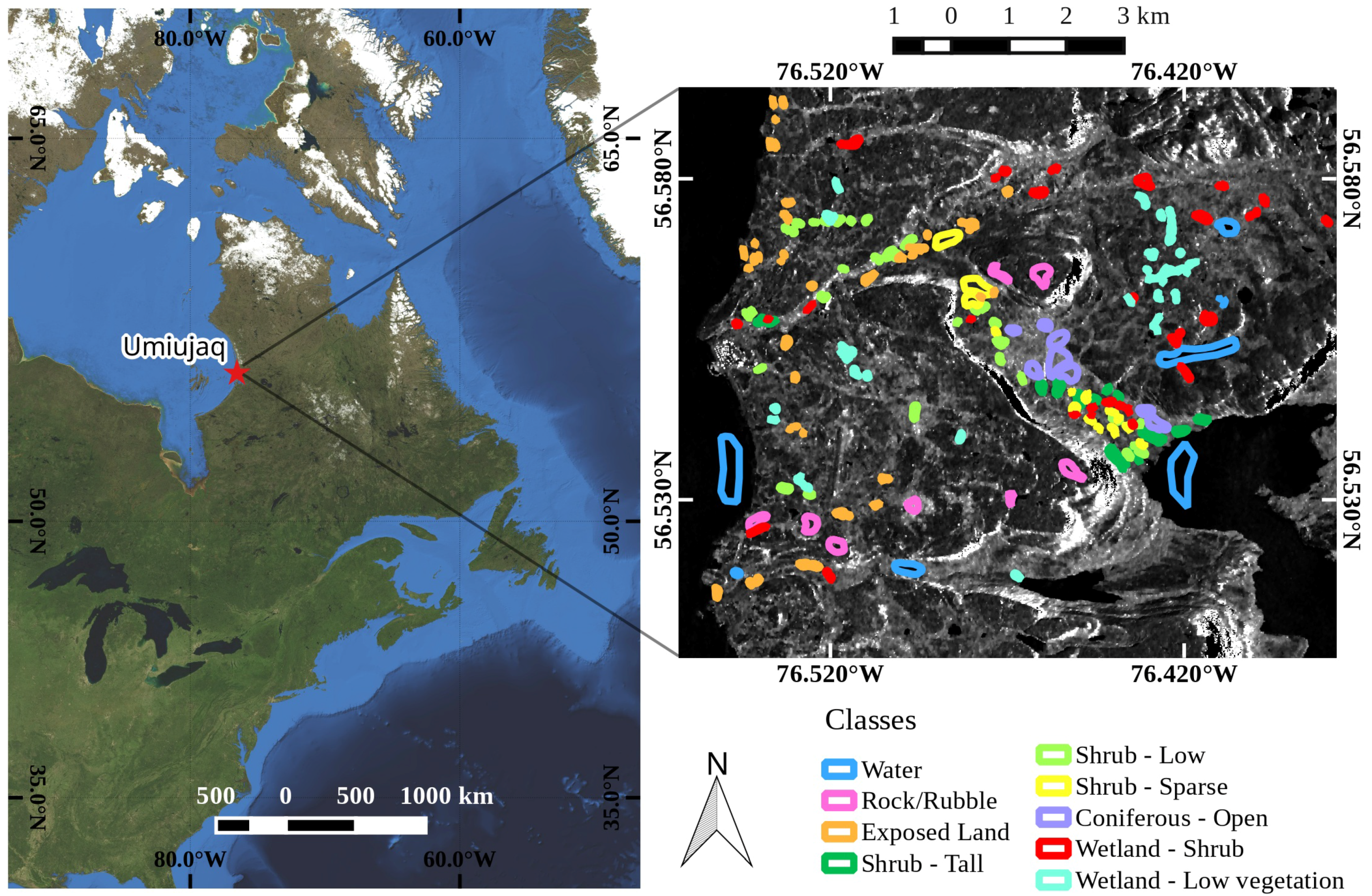
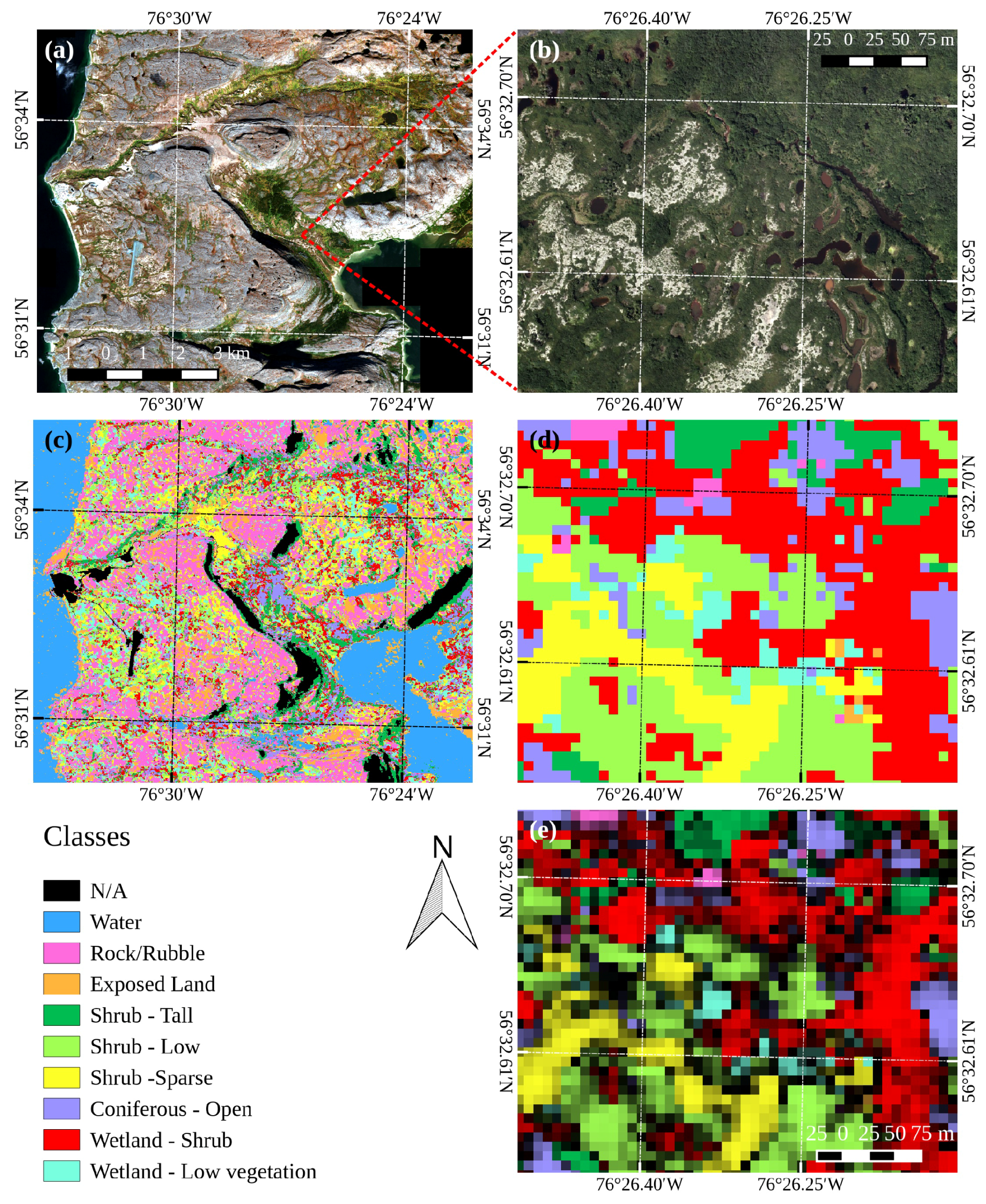
2.1. Study Area
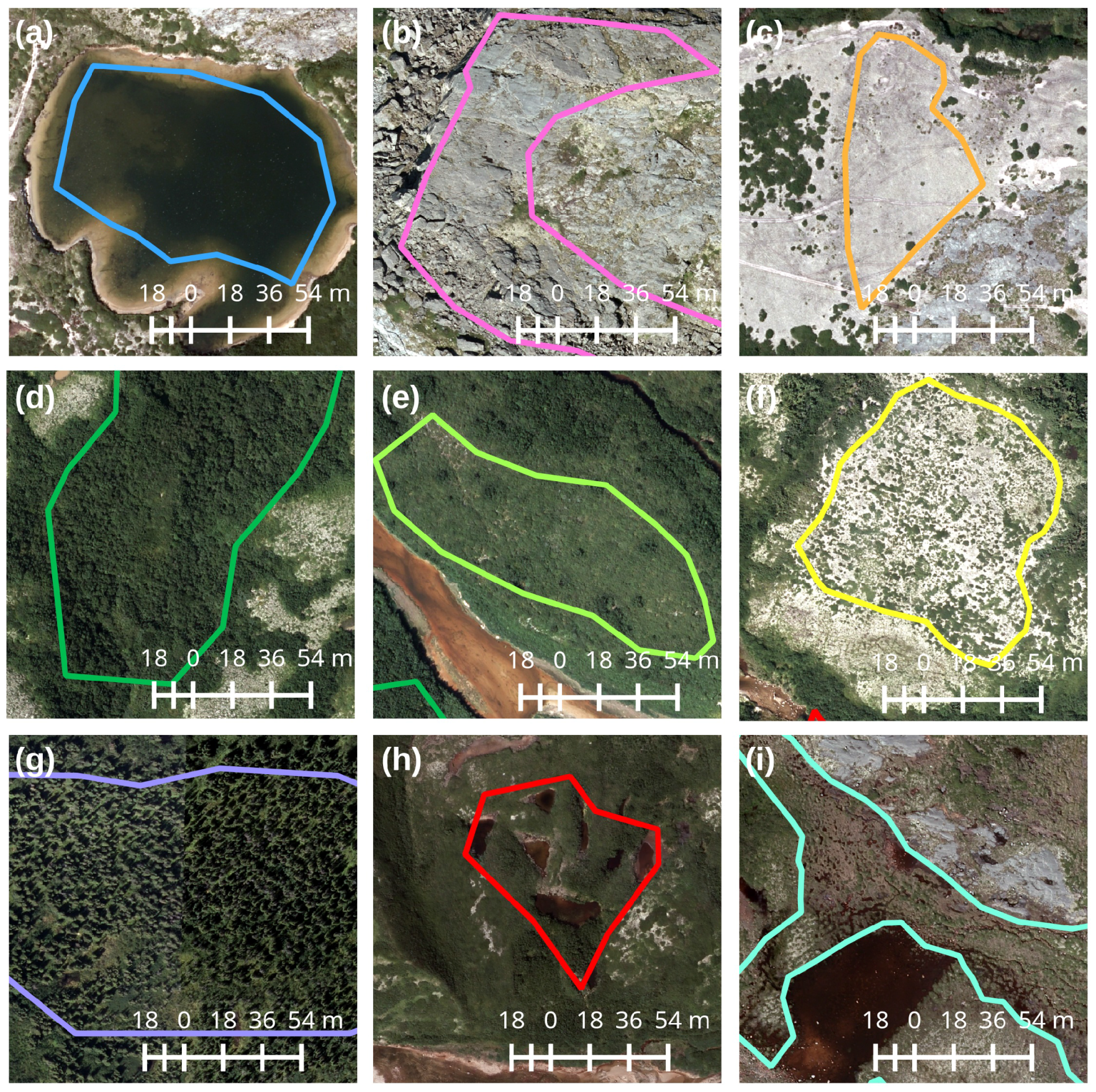
2.2. Satellite, GIS and In Situ Datasets
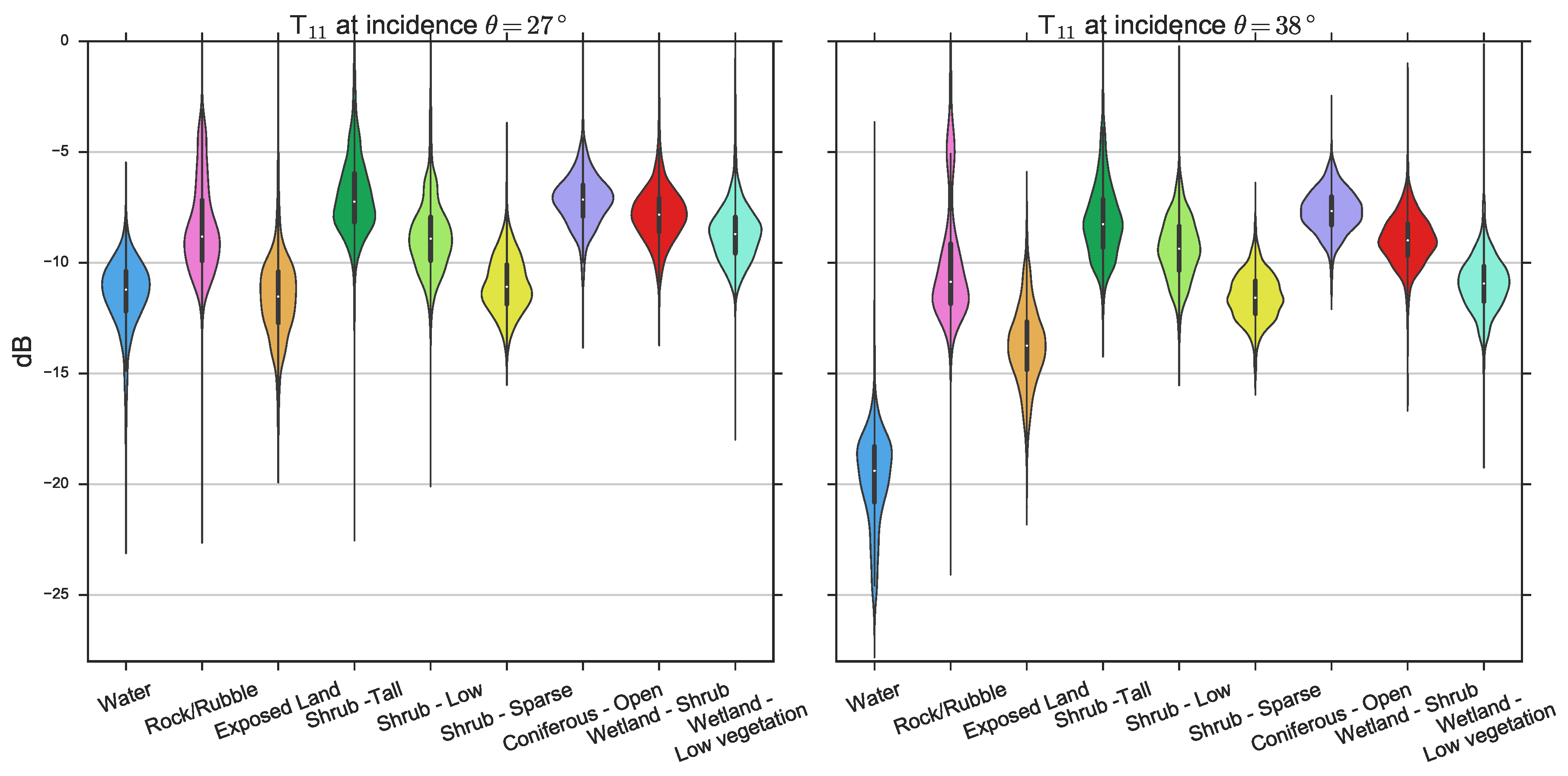
2.2.1. SAR Processing
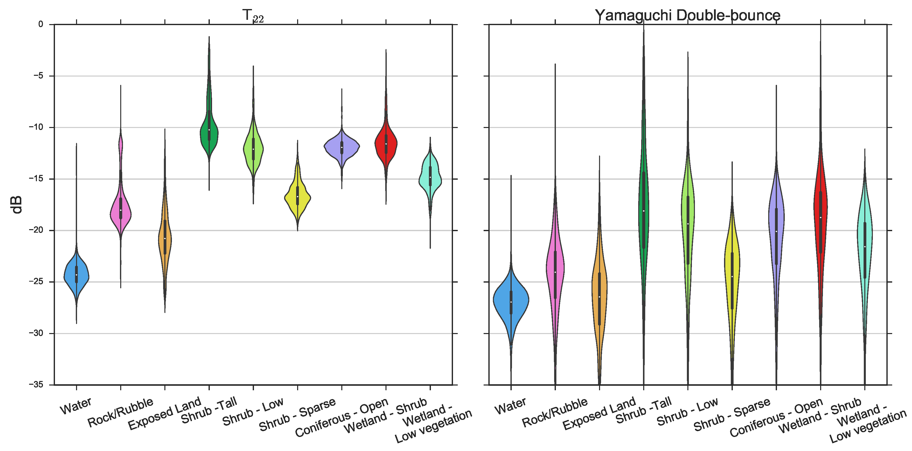
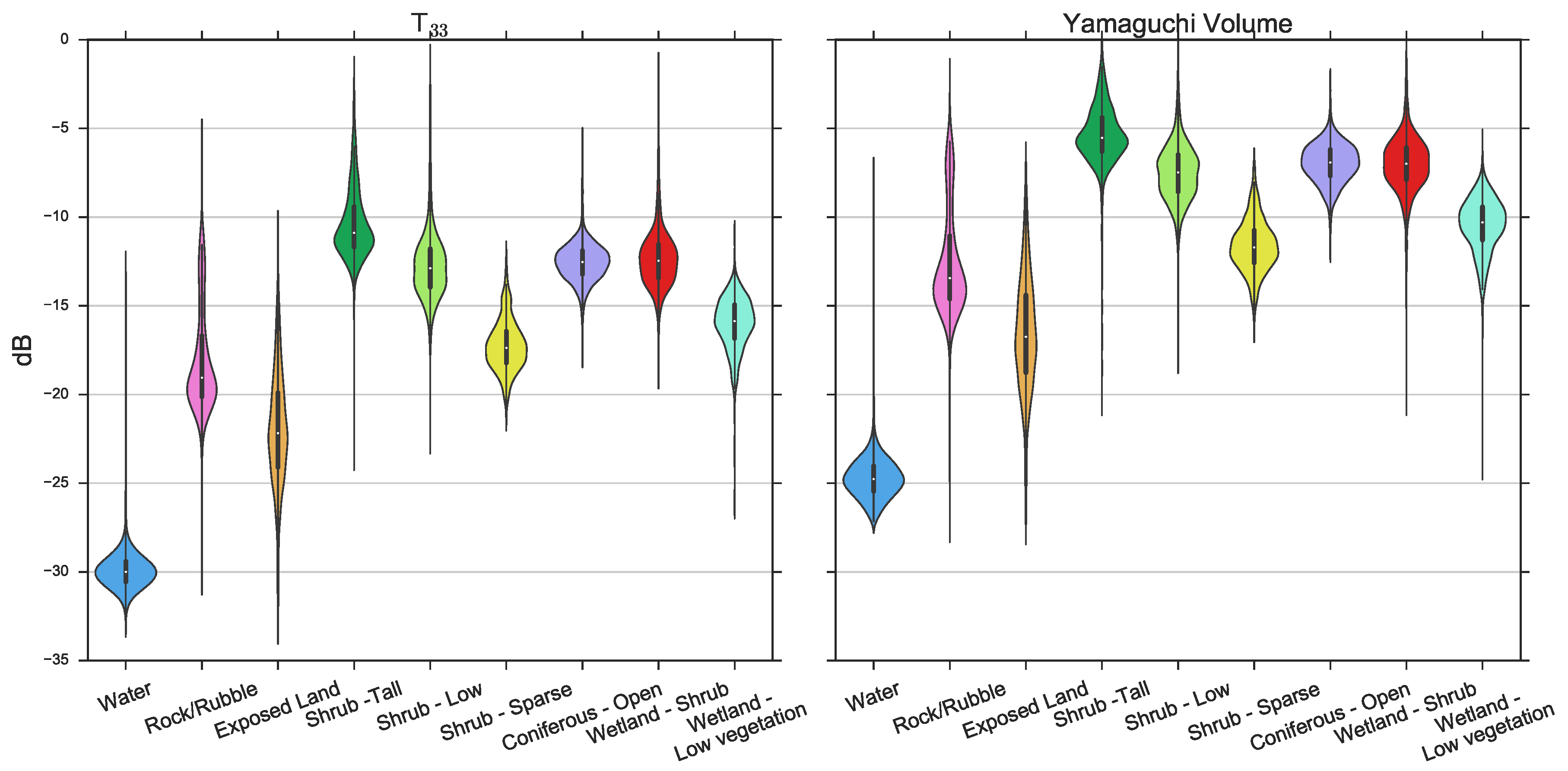
2.2.2. Polarimetric Decompositions
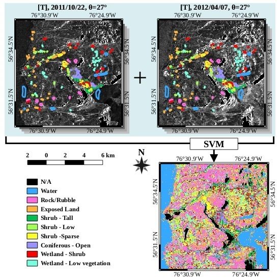
2.3. Classification
3. Results
3.1. Classification with a Single Image
3.2. Classification with Multiple Images
4. Discussion
4.1. Classification with a Single Image
4.2. Classification with Multiple Images
5. Conclusions
Acknowledgments
Author Contributions
Conflicts of Interest
References
- Sturm, M.; Holmgren, J.; McFadden, J.P.; Liston, G.E.; Chapin, F.S.; Racine, C.H. Snow-Shrub Interactions in Arctic Tundra: A Hypothesis with Climatic Implications. J. Clim. 2001, 14, 336–344. [Google Scholar] [CrossRef]
- Sturm, M.; Schimel, J.; Michaelson, G.; Welker, J.; Oberbauer, S.; Liston, G.; Fahnestock, J.; Romanovsky, V.E. Winter biological processes could help convert Arctic tundra to shrubland. BioScience 2005, 55, 17–26. [Google Scholar] [CrossRef]
- Myers-Smith, I.H.; Forbes, B.C.; Wilmking, M.; Hallinger, M.; Lantz, T.; Blok, D.; Tape, K.D.; Macias-Fauria, M.; Sass-Klaassen, U.; Lévesque, E.; et al. Shrub expansion in tundra ecosystems: Dynamics, impacts and research priorities. Environ. Res. Lett. 2011, 6, 045509. [Google Scholar] [CrossRef]
- Elmendorf, S.C.; Henry, G.H.R.; Hollister, R.D.; Bjork, R.G.; Boulanger-Lapointe, N.; Cooper, E.J.; Cornelissen, J.H.C.; Day, T.A.; Dorrepaal, E.; Elumeeva, T.G.; et al. Plot-scale evidence of tundra vegetation change and links to recent summer warming. Nat. Clim. Chang. 2012, 2, 453–457. [Google Scholar] [CrossRef]
- Sturm, M.; Racine, C.; Tape, K. Climate change: Increasing shrub abundance in the Arctic. Nature 2001, 411, 546–547. [Google Scholar] [CrossRef] [PubMed]
- Tremblay, B.; Lévesque, E.; Boudreau, S. Recent expansion of erect shrubs in the Low Arctic: Evidence from Eastern Nunavik. Environ. Res. Lett. 2012, 7, 035501. [Google Scholar] [CrossRef]
- Cornelissen, J.H.C.; Callaghan, T.V.; Alatalo, J.M.; Michelsen, A.; Graglia, E.; Hartley, A.E.; Hik, D.S.; Hobbie, S.E.; Press, M.C.; Robinson, C.H.; et al. Global change and Arctic ecosystems: is lichen decline a function of increases in vascular plant biomass? J. Ecol. 2001, 89, 984–994. [Google Scholar] [CrossRef]
- Provencher-Nolet, L.; Bernier, M.; Lévesque, E. Quantification des changements récents à l’écotone forêt-toundra à partir de l’analyse numérique de photographies aériennes. Écoscience 2014, 21, 419–433. [Google Scholar] [CrossRef]
- Forbes, B.C.; Fauria, M.M.; Zetterberg, P. Russian Arctic warming and ”greening” are closely tracked by tundra shrub willows. Glob. Chang. Biol. 2009, 16, 1542–1554. [Google Scholar] [CrossRef]
- Hallinger, M.; Manthey, M.; Wilmking, M. Establishing a missing link: Warm summers and winter snow cover promote shrub expansion into alpine tundra in Scandinavia. New Phytol. 2010, 186, 890–899. [Google Scholar] [CrossRef] [PubMed]
- Buckeridge, K.M.; Grogan, P. Deepened snow alters soil microbial nutrient limitations in Arctic birch hummock tundra. Appl. Soil Ecol. 2008, 39, 210–222. [Google Scholar] [CrossRef]
- Schimel, J.P.; Bilbrough, C.; Welker, J.M. Increased snow depth affects microbial activity and nitrogen mineralization in two Arctic tundra communities. Soil Biol. Biochem. 2004, 36, 217–227. [Google Scholar] [CrossRef]
- Olthof, I.; Pouliot, D. Treeline vegetation composition and change in Canada’s western SubArctic from AVHRR and canopy reflectance modeling. Remote Sens. Environ. 2010, 114, 805–815. [Google Scholar] [CrossRef]
- Chasmer, L.; Kenward, A.; Quinton, W.; Petrone, R. CO2 exchanges within zones of rapid conversion from permafrost plateau to bog and fen land cover types. Arct. Antarct. Alp. Res. 2012, 44, 399–411. [Google Scholar] [CrossRef]
- Fraser, R.H.; Lantz, T.C.; Olthof, I.; Kokelj, S.V.; Sims, R.A. Warming-Induced Shrub Expansion and Lichen Decline in the Western Canadian Arctic. Ecosystems 2014, 17, 1151–1168. [Google Scholar] [CrossRef]
- Stow, D.A.; Hope, A.; McGuire, D.; Verbyla, D.; Gamon, J.; Huemmrich, F.; Houston, S.; Racine, C.; Sturm, M.; Tape, K.; et al. Remote sensing of vegetation and land-cover change in Arctic Tundra Ecosystems. Remote Sens. Environ. 2004, 89, 281–308. [Google Scholar] [CrossRef]
- Blok, D.; Schaepman-Strub, G.; Bartholomeus, H.; Heijmans, M.M.P.D.; Maximov, T.C.; Berendse, F. The response of Arctic vegetation to the summer climate: Relation between shrub cover, NDVI, surface albedo and temperature. Environ. Res. Lett. 2011, 6, 035502. [Google Scholar] [CrossRef]
- Boelman, N.T.; Gough, L.; McLaren, J.R.; Greaves, H. Does NDVI reflect variation in the structural attributes associated with increasing shrub dominance in Arctic tundra? Environ. Res. Lett. 2011, 6, 035501. [Google Scholar] [CrossRef]
- McManus, K.M.; Morton, D.C.; Masek, J.G.; Wang, D.; Sexton, J.O.; Nagol, J.R.; Ropars, P.; Boudreau, S. Satellite-based evidence for shrub and graminoid tundra expansion in northern Quebec from 1986 to 2010. Glob. Chang. Biol. 2012, 18, 2313–2323. [Google Scholar] [CrossRef]
- Ropars, P.; Boudreau, S. Shrub expansion at the forest-tundra ecotone: Spatial heterogeneity linked to local topography. Environ. Res. Lett. 2012, 7, 015501. [Google Scholar] [CrossRef]
- Hope, A.S.; Pence, K.R.; Stow, D.A. NDVI from low altitude aircraft and composited NOAA AVHRR data for scaling Arctic ecosystem fluxes. Int. J. Remote Sens. 2004, 25, 4237–4250. [Google Scholar] [CrossRef]
- Musick, H.; Schaber, G.S.; Breed, C.S. AIRSAR studies of woody shrub density in Semiarid Rangeland: Jornada del Muerto, New Mexico. Remote Sens. Environ. 1998, 66, 29–40. [Google Scholar] [CrossRef]
- Svoray, T.; Shoshany, M.; Curran, P.J.; Foody, G.M.; Perevolotsky, A. Relationship between green leaf biomass volumetric density and ERS-2 SAR backscatter of four vegetation formations in the semi-arid zone of Israel. Int. J. Remote Sens. 2001, 22, 1601–1607. [Google Scholar] [CrossRef]
- Patel, P.; Srivastava, H.S.; Panigrahy, S.; Parihar, J.S. Comparative evaluation of the sensitivity of multi-polarized multi-frequency SAR backscatter to plant density. Int. J. Remote Sens. 2006, 27, 293–305. [Google Scholar] [CrossRef]
- Monsivais-Huertero, A.; Chenerie, I.; Sarabandi, K. Sahelian-grassland parameter estimation from backscattered radar response. IEEE Int. Geosci. Remote Sens. Symp. 2008, 3, 1119–1122. [Google Scholar]
- Duguay, Y.; Bernier, M.; Lévesque, E.; Tremblay, B. Potential of C and X band SAR for shrub growth monitoring in sub-arctic environments. Remote Sens. 2015, 7, 9410–9430. [Google Scholar] [CrossRef]
- Cloude, S.R.; Pottier, E. A review of target decomposition theorems in radar polarimetry. IEEE Trans. Geosci. Remote Sens. 1996, 34, 498–518. [Google Scholar] [CrossRef]
- Yamaguchi, Y.; Moriyama, T.; Ishido, M.; Yamada, H. Four-component scattering model for polarimetric SAR image decomposition. IEEE Trans. Geosci. Remote Sens. 2005, 43, 1699–1706. [Google Scholar] [CrossRef]
- Cloude, S.R.; Pottier, E. An entropy based classification scheme for land applications of polarimetric SAR. IEEE Trans. Geosci. Remote Sens. 1997, 35, 68–78. [Google Scholar] [CrossRef]
- Brouillet, L.; Coursol, F.; Meades, S.J.; Favreau, M.; Anions, M.; Bélisle, P.; Desmet, P. VASCAN, Database of Vascular Plants of Canada. Available online: http://data.canadensys.net/vascan (accessed on 8 June 2016).
- Freeman, A.; Durden, S.L. A three-component scattering model for polarimetric SAR data. IEEE Trans. Geosci. Remote Sens. 1998, 36, 963–973. [Google Scholar] [CrossRef]
- PolSARpro Version 5.0. Available online: https://earth.esa.int/web/polsarpro (accessed on 8 June 2016).
- Lee, J.S.; Wen, J.H.; Ainsworth, T.L.; Chen, K.S.; Chen, A.J. Improved Sigma Filter for Speckle Filtering of SAR Imagery. IEEE Trans. Geosci. Remote Sens. 2009, 47, 202–213. [Google Scholar]
- López-Martínez, C.; Pottier, E.; Cloude, S.R. Statistical Assessment of eigenvector-based target decomposition theorems in radar polarimetry. IEEE Trans. Geosci. Remote Sens. 2005, 43, 2058–2074. [Google Scholar] [CrossRef]
- MapReady. Available online: https://www.asf.alaska.edu/data-tools/mapready (accessed on 8 June 2016).
- Wulder, M.; Nelson, T. EOSD Land Cover Classification Legend Report; Natural Resources Canada, Canadian Forest Service, Pacific Forestry Centre: Victoria, BC, Canada, 2003. [Google Scholar]
- Burges, C. A tutorial on support vector machines for pattern recognition. Data Min. Knowl. Discov. 1998, 2, 121–167. [Google Scholar] [CrossRef]
- Huang, C.; Davis, L.S.; Townshend, J.R.G. An assessment of support vector machines for land cover classification. Int. J. Remote Sens. 2002, 23, 725–749. [Google Scholar] [CrossRef]
- Foody, G.M.; Mathur, A. A relative evaluation of multiclass image classification by support vector machines. IEEE Trans. Geosci. Remote Sens. 2004, 42, 1335–1343. [Google Scholar] [CrossRef]
- Mountrakis, G.; Im, J.; Ogole, C. Support vector machines in remote sensing: A review. ISPRS J. Photogramm. Remote Sens. 2011, 66, 247–259. [Google Scholar] [CrossRef]
- Fukuda, S.; Hirosawa, H. Support vector machine classification of land cover: Application to polarimetric SAR data. IEEE Int. Geosci. Remote Sens. Symp. 2001, 1, 187–189. [Google Scholar]
- Lee, J.S.; Hoppel, K.W.; Mango, S.A.; Miller, A.R. Intensity and phase statistics of multilook polarimetric and interferometric SAR imagery. IEEE Trans. Geosci. Remote Sens. 1994, 32, 1017–1028. [Google Scholar]
- Lardeux, C.; Frison, P.L.; Tison, C.; Souyris, J.C.; Stoll, B.; Fruneau, B.; Rudant, J.P. Support vector machine for multifrequency SAR polarimetric data classification. IEEE Trans. Geosci. Remote Sens. 2009, 47, 4143–4152. [Google Scholar] [CrossRef]
- Zhang, L.; Zou, B.; Zhang, J.; Zhang, Y. Classification of Polarimetric SAR Image Based on Support Vector Machine Using Multiple-component Scattering Model and Texture Features. EURASIP J. Adv. Signal Process. 2010, 2010, 1–9. [Google Scholar] [CrossRef]
- Longepe, N.; Rakwatin, P.; Isoguchi, O.; Shimada, M.; Uryu, Y.; Yulianto, K. Assessment of ALOS PALSAR 50 m orthorectified FBD data for regional land cover classification by support vector machines. IEEE Trans. Geosci. Remote Sens. 2011, 49, 2135–2150. [Google Scholar] [CrossRef]
- Tan, C.P.; Koay, J.Y.; Lim, K.S.; Ewe, H.T.; Chuah, H.T. Classification of multi-temporal SAR images for rice crops using combined entropy decomposition and support vector machine technique. Prog. Electromagn. Res. 2007, 71, 19–39. [Google Scholar] [CrossRef]
- Longépé, N.; Shimada, M.; Allain, S.; Pottier, E. Capabilities of full-polarimetric palsar/alos for snowextent mapping. IEEE Int. Geosci. Remote Sens. Symp. 2008, 4, 1026–1029. [Google Scholar]
- Li, Z.; Huang, L.; Chen, Q.; Tian, B. Glacier snowline detection on a polarimetric SAR image. IEEE Geosci. Remote Sens. Lett. 2012, 9, 584–588. [Google Scholar]
- Liu, H.; Guo, H.; Zhang, L. SVM-Based Sea Ice Classification Using Textural Features and Concentration From RADARSAT-2 Dual-Pol ScanSAR Data. IEEE J. Sel. Top. Appl. Earth Obs. Remote Sens. 2015, 8, 1601–1613. [Google Scholar] [CrossRef]
- Lardeux, C.; Frison, P.L.; Tison, C.; Souyris, J.C.; Stoll, B.; Fruneau, B.; Rudant, J.P. Classification of Tropical Vegetation Using Multifrequency Partial SAR Polarimetry. IEEE Geosci. Remote Sens. Lett. 2011, 8, 133–137. [Google Scholar] [CrossRef]
- Neumann, M.; Saatchi, S.; Ulander, L.M.H.; Fransson, J.E.S. Assessing performance of L- and P-band polarimetric interferometric SAR data in estimating boreal forest above-ground biomass. IEEE Trans. Geosci. Remote Sens. 2012, 50, 714–726. [Google Scholar] [CrossRef]
- Ulaby, F.T.; Moore, R.K.; Fung, A.K. From theory to applications. In Microwave Remote Sensing Active and Passive; Addison-Wesley: Reading, MA, USA, 1986; Volume 3. [Google Scholar]
- De Almeida Furtado, L.F.; Silva, T.S.F.; de Moraes Novo, E.M.L. Dual-season and full-polarimetric C band SAR assessment for vegetation mapping in the Amazon várzea wetlands. Remote Sens. Environ. 2016, 174, 212–222. [Google Scholar] [CrossRef]
- Orfeo Toolbox. Available online: https://www.orfeo-toolbox.org (accessed on 8 June 2016).
- Chang, C.C.; Lin, C.J. LIBSVM: A library for support vector machines. ACM Trans. Intell. Syst. Tech. 2011, 2. [Google Scholar] [CrossRef]
- Wu, T.F.; Lin, C.J.; Weng, R.C. Probability Estimates for Multi-class Classification by Pairwise Coupling. J. Mach. Learn. Res. 2004, 5, 975–1005. [Google Scholar]
- Duguay, Y.; Bernier, M. The use of RADARSAT-2 and TerraSAR-X data for the evaluation of snow characteristics in sub-Arctic regions. In Proceedings of the 2012 IEEE International Geoscience and Remote Sensing Symposium (IGARSS), Munich, Germany, 22–27 July 2012; pp. 3556–3559.


| Date | Sensor | Polarizations | Incidence Angle (θ) |
|---|---|---|---|
| 2011/10/19 | RADARSAT-2 | quad-pol | 38 |
| 2011/10/22 | RADARSAT-2 | quad-pol | 27 |
| 2011/11/12 | RADARSAT-2 | quad-pol | 38 |
| 2011/11/15 | RADARSAT-2 | quad-pol | 27 |
| 2011/12/06 | RADARSAT-2 | quad-pol | 38 |
| 2011/12/09 | RADARSAT-2 | quad-pol | 27 |
| 2012/03/11 | RADARSAT-2 | quad-pol | 38 |
| 2012/03/14 | RADARSAT-2 | quad-pol | 27 |
| 2012/04/04 | RADARSAT-2 | quad-pol | 38 |
| 2012/04/07 | RADARSAT-2 | quad-pol | 27 |
| Classes | 0 | 1 | 2 | 3 | 4 | 5 | 6 | 7 |
|---|---|---|---|---|---|---|---|---|
| Height (m) | 0 | 0–0.25 | 0.25–0.50 | 0.50–1 | 1–1.5 | 1.5–2.5 | 2.5–5 | >5 |
| Coverage (%) | 0 | 0–5 | 5–15 | 15–25 | 25–50 | 50–75 | 75–90 | 90–100 |
| Class | Symbol | Number of Training Polygons | Total Area of Training Polygons (m) | Description |
|---|---|---|---|---|
| Water | W | 8 | 926,900 | Lakes, rivers, ponds larger than 3 × 3 pixels (27 × 27 m) |
| Rock/Rubble | R | 8 | 317,900 | Exposed bedrock, block field or rubble |
| Exposed Land | EL | 36 | 204,800 | Exposed soil, mostly sand |
| Shrub-Tall | ST | 14 | 216,800 | Covered with at least 50% shrub; average shrub height greater than or equal to 1 m. |
| Shrub-Low | SL | 33 | 194,500 | Covered with at least 50% shrub; average shrub height less than 1 m. |
| Shrub-Sparse | SS | 16 | 248,800 | Covered with less than 50% shrub, regardless of shrub height; lichen and herbaceous vegetation cover at least 50% of the ground. |
| Coniferous-Open | CO | 9 | 409,000 | 25%–50% crown closure; coniferous trees make up 75% or more of the stands. |
| Wetland-Shrub | WS | 31 | 230,000 | Land with a water table near, at or above the soil surface for enough time to promote wetland or aquatic processes, the vegetation is composed in the majority of low or tall shrubs. This can also be composed of smallponds(less than 3 × 3 pixels) surrounded by shrubs. |
| Wetland-Low vegetation | WL | 36 | 210,100 | Land with a water table near, at or above the soil surface for enough time to promote wetland or aquatic processes; the vegetation is composed in the majority of mosses, herbs and some prostrate shrub. This is generally composed of peatlands with small ponds (less than 3 × 3 pixels). |
| Matrix | Model-Based | Eigenvalue-Based | |||||
|---|---|---|---|---|---|---|---|
| Date | Incidence Angle | Accuracy | Accuracy | Accuracy | |||
| 2011/10/19 | 38 | 74.9% | 0.72 | 66.8% | 0.63 | 65.1% | 0.61 |
| 2011/10/22 | 27 | 74.9% | 0.72 | 67.2% | 0.63 | 66.9% | 0.63 |
| 2011/11/12 | 38 | 70.0% | 0.66 | 63.9% | 0.59 | 62.3% | 0.58 |
| 2011/11/15 | 27 | 66.9% | 0.63 | 58.2% | 0.53 | 56.7% | 0.51 |
| 2011/12/06 | 38 | 64.4% | 0.60 | 56.8% | 0.51 | 54.4% | 0.49 |
| 2011/12/09 | 27 | 65.9% | 0.62 | 55.9% | 0.50 | 55.4% | 0.50 |
| 2012/03/11 | 38 | 58.4% | 0.53 | 44.3% | 0.37 | 49.0% | 0.43 |
| 2012/03/14 | 27 | 54.6% | 0.49 | 43.1% | 0.36 | 44.7% | 0.38 |
| 2012/04/04 | 38 | 60.7% | 0.56 | 46.5% | 0.40 | 50.0% | 0.44 |
| 2012/04/07 | 27 | 58.9% | 0.54 | 45.6% | 0.39 | 46.2% | 0.39 |
| Matrix | Model-Based | Eigenvalue-Based | ||||
|---|---|---|---|---|---|---|
| Class | Producer’s Accuracy | User’s Accuracy | Producer’s Accuracy | User’s Accuracy | Producer’s Accuracy | User’s Accuracy |
| Water | 98.7% | 95.8% | 99.1% | 94.9% | 75.6% | 80.3% |
| Rock/Rubble | 79.4% | 75.7% | 72.8% | 71.7% | 25.9% | 41.3% |
| Exposed Land | 81.2% | 86.8% | 77.4% | 89.7% | 60.4% | 59.2% |
| Shrub-Tall | 77.2% | 69.3% | 70.2% | 57.0% | 53.9% | 48.3% |
| Shrub-Low | 60.4% | 68.2% | 52.7% | 49.9% | 45.3% | 41.8% |
| Shrub-Sparse | 80.0% | 81.4% | 75.6% | 79.0% | 69.2% | 53.9% |
| Coniferous-Open | 70.1% | 62.2% | 61.9% | 52.4% | 66.7% | 55.8% |
| Wetland-Shrub | 47.6% | 58.7% | 19.8% | 38.5% | 25.2% | 38.4% |
| Wetland-Low Vegetation | 79.7% | 75.5% | 75.4% | 67.1% | 66.8% | 62.6% |
| Predicted | W | R | EL | ST | SL | SS | CO | WS | WL | Total | |
|---|---|---|---|---|---|---|---|---|---|---|---|
| Reference | |||||||||||
| W | 1163 | 0 | 13 | 0 | 0 | 1 | 0 | 0 | 1 | 1178 | |
| R | 2 | 955 | 89 | 5 | 3 | 34 | 39 | 6 | 70 | 1203 | |
| EL | 49 | 93 | 967 | 1 | 4 | 71 | 0 | 1 | 5 | 1191 | |
| ST | 0 | 0 | 0 | 929 | 68 | 0 | 88 | 118 | 0 | 1203 | |
| SL | 0 | 7 | 2 | 118 | 711 | 28 | 130 | 93 | 88 | 1177 | |
| SS | 0 | 78 | 42 | 1 | 28 | 949 | 1 | 0 | 87 | 1186 | |
| CO | 0 | 24 | 0 | 92 | 59 | 1 | 860 | 163 | 28 | 1227 | |
| WS | 0 | 13 | 0 | 194 | 121 | 1 | 261 | 562 | 29 | 1181 | |
| WL | 0 | 91 | 1 | 1 | 49 | 81 | 4 | 14 | 947 | 1188 | |
| Total | 1214 | 1261 | 1114 | 1341 | 1043 | 1166 | 1383 | 957 | 1255 | 10,734 | |
| Dates | Incidence Angles | Accuracy | κ |
|---|---|---|---|
| 2011/10/19 + 2011/10/22 | 27 + 38 | 89.0% | 0.88 |
| 2011/11/12 + 2011/11/15 | 27 + 38 | 85.8% | 0.84 |
| 2011/12/06 + 2011/12/09 | 27 + 38 | 80.2% | 0.78 |
| 2012/03/11 + 2012/03/14 | 27 + 38 | 74.8% | 0.72 |
| 2012/04/04 + 2012/04/07 | 27 + 38 | 78.1% | 0.75 |
| First Date | Second Date | Accuracy | Accuracy | ||
|---|---|---|---|---|---|
| 2011/10 | 2011/11 | 89.4% | 0.88 | 87.0% | 0.85 |
| 2011/10 | 2011/12 | 88.2% | 0.87 | 86.6% | 0.85 |
| 2011/10 | 2012/03 | 88.4% | 0.87 | 87.3% | 0.86 |
| 2011/10 | 2012/04 | 90.1% | 0.89 | 88.2% | 0.87 |
| 2011/11 | 2011/12 | 86.9% | 0.85 | 85.0% | 0.83 |
| 2011/11 | 2012/03 | 84.4% | 0.82 | 85.8% | 0.84 |
| 2011/11 | 2012/04 | 84.7% | 0.83 | 86.7% | 0.85 |
| 2011/12 | 2012/03 | 84.3% | 0.82 | 84.0% | 0.82 |
| 2011/12 | 2012/04 | 86.3% | 0.85 | 83.7% | 0.82 |
| 2012/03 | 2012/04 | 79.2% | 0.77 | 79.9% | 0.77 |
| Multi-Angle | Multi-Date | |||
|---|---|---|---|---|
| Class | Producer’s Accuracy | User’s Accuracy | Producer’s Accuracy | User’s Accuracy |
| Water | 99.7% | 99.5% | 98.4% | 97.6% |
| Rock/Rubble | 90.8% | 88.7% | 87.5% | 89.0% |
| Exposed Land | 90.4% | 95.0% | 85.2% | 91.4% |
| Shrub-Tall | 90.9% | 82.1% | 93.4% | 85.0% |
| Shrub-Low | 82.7% | 88.2% | 86.1% | 89.4% |
| Shrub-Sparse | 92.2% | 90.9% | 93.8% | 92.1% |
| Coniferous-Open | 87.7% | 89.8% | 90.4% | 88.2% |
| Wetland-Shrub | 75.7% | 80.0% | 82.0% | 86.1% |
| Wetland-Low Vegetation | 90.9% | 87.6% | 93.6% | 92.3% |
| Predicted | W | R | EL | ST | SL | SS | CO | WS | WL | Total | |
|---|---|---|---|---|---|---|---|---|---|---|---|
| Reference | |||||||||||
| W | 1175 | 0 | 3 | 0 | 0 | 0 | 0 | 0 | 0 | 1178 | |
| R | 1 | 1080 | 39 | 17 | 1 | 17 | 4 | 1 | 30 | 1190 | |
| EL | 5 | 64 | 1072 | 1 | 1 | 32 | 0 | 1 | 10 | 1186 | |
| ST | 0 | 0 | 0 | 1093 | 32 | 0 | 19 | 59 | 0 | 1203 | |
| SL | 0 | 1 | 1 | 49 | 968 | 22 | 24 | 66 | 40 | 1171 | |
| SS | 0 | 26 | 10 | 0 | 11 | 1099 | 1 | 1 | 44 | 1192 | |
| CO | 0 | 1 | 0 | 48 | 14 | 0 | 1081 | 88 | 0 | 1232 | |
| WS | 0 | 0 | 0 | 122 | 61 | 0 | 74 | 887 | 28 | 1172 | |
| WL | 0 | 45 | 4 | 2 | 10 | 39 | 1 | 6 | 1074 | 1181 | |
| Total | 1181 | 1217 | 1129 | 1332 | 1098 | 1209 | 1204 | 1109 | 1226 | 10,705 | |
| Predicted | W | R | EL | ST | SL | SS | CO | WS | WL | Total | |
|---|---|---|---|---|---|---|---|---|---|---|---|
| Reference | |||||||||||
| W | 1162 | 0 | 14 | 4 | 0 | 1 | 0 | 0 | 0 | 1181 | |
| R | 0 | 1047 | 63 | 34 | 7 | 9 | 6 | 3 | 28 | 1197 | |
| EL | 28 | 80 | 1007 | 7 | 5 | 47 | 0 | 2 | 6 | 1182 | |
| ST | 0 | 1 | 0 | 1127 | 18 | 0 | 19 | 41 | 0 | 1206 | |
| SL | 0 | 3 | 0 | 41 | 1001 | 9 | 38 | 55 | 15 | 1162 | |
| SS | 0 | 8 | 11 | 0 | 9 | 1112 | 3 | 3 | 39 | 1185 | |
| CO | 0 | 5 | 0 | 39 | 20 | 5 | 1111 | 48 | 1 | 1229 | |
| WS | 0 | 8 | 1 | 74 | 52 | 0 | 75 | 978 | 4 | 1192 | |
| WL | 0 | 25 | 6 | 0 | 8 | 24 | 7 | 6 | 1115 | 1191 | |
| Total | 1190 | 1177 | 1102 | 1326 | 1120 | 1207 | 1259 | 1136 | 1208 | 10,725 | |
© 2016 by the authors; licensee MDPI, Basel, Switzerland. This article is an open access article distributed under the terms and conditions of the Creative Commons Attribution (CC-BY) license (http://creativecommons.org/licenses/by/4.0/).
Share and Cite
Duguay, Y.; Bernier, M.; Lévesque, E.; Domine, F. Land Cover Classification in SubArctic Regions Using Fully Polarimetric RADARSAT-2 Data. Remote Sens. 2016, 8, 697. https://doi.org/10.3390/rs8090697
Duguay Y, Bernier M, Lévesque E, Domine F. Land Cover Classification in SubArctic Regions Using Fully Polarimetric RADARSAT-2 Data. Remote Sensing. 2016; 8(9):697. https://doi.org/10.3390/rs8090697
Chicago/Turabian StyleDuguay, Yannick, Monique Bernier, Esther Lévesque, and Florent Domine. 2016. "Land Cover Classification in SubArctic Regions Using Fully Polarimetric RADARSAT-2 Data" Remote Sensing 8, no. 9: 697. https://doi.org/10.3390/rs8090697
APA StyleDuguay, Y., Bernier, M., Lévesque, E., & Domine, F. (2016). Land Cover Classification in SubArctic Regions Using Fully Polarimetric RADARSAT-2 Data. Remote Sensing, 8(9), 697. https://doi.org/10.3390/rs8090697