Article

Maximum Likelihood Deconvolution of Beamformed Images with Signal-Dependent Speckle Fluctuations from Gaussian Random Fields: With Application to Ocean Acoustic Waveguide Remote Sensing (OAWRS)

Department of Mechanical Engineering, Massachusetts Institute of Technology, Cambridge, MA 02139, USA
*
Author to whom correspondence should be addressed.
Remote Sens. 2016, 8(9), 694; https://doi.org/10.3390/rs8090694
Submission received: 30 June 2016 / Revised: 12 August 2016 / Accepted: 17 August 2016 / Published: 23 August 2016
(This article belongs to the Special Issue Underwater Acoustic Remote Sensing)

Abstract

:
Wide area acoustic remote sensing often involves the use of coherent receiver arrays to determine the spatial distribution of sources and scatterers at any instant. The resulting acoustic intensity images are typically corrupted by signal-dependent noise from Gaussian random field fluctuations arising from the central limit theorem and have a spatial resolution that depends on the incident direction, sensing array aperture and wavelength. Here, we use the maximum likelihood method to deconvolve the intensity distribution measured on a coherent line array assuming a discrete angular distribution of incident plane waves. Instantaneous wide area population density images of fish aggregations measured with Ocean Acoustic Waveguide Remote Sensing (OAWRS) are deconvolved to illustrate the effectiveness of this approach in improving angular resolution over conventional planewave beamforming.

Graphical Abstract

1. Introduction

Coherent receiver arrays are often used to generate acoustic images of the undersea environment to chart the spatial distribution of acoustic scatterers or sources, such as fish, marine mammals, plankton, submerged objects and bathymetric features [1,2,3]. In a typical wide-area application, such as Ocean Acoustic Waveguide Remote Sensing (OAWRS), involving a horizontal, coherent line array, an acoustic image is formed by charting the acoustic intensity received from scatterers or sources in range by travel time analysis and in azimuth by plane-wave beam forming [4,5,6,7]. Conventional time-harmonic plane wave beamforming [2,3] on a line array by Fourier transform from the spatial to the wavenumber domain can non-linearly blur the angular distribution of incident plane waves for array geometries that lack spherical symmetry due to the nonlinear relationship between the incident direction and wavenumber components along the array caused by foreshortening.
Here, we develop and apply a maximum likelihood (ML) approach for the spatial deconvolution of acoustic intensity images generated by a coherent acoustic array. We take advantage of the relatively pervasive circular complex Gaussian random (CCGR) statistics of acoustic fields in the ocean that follow from the central limit theorem for many typical scenarios of propagation, radiation or scattering [4,5,6,8,9,10,11,12,13,14]. Instantaneous intensity then follows a negative exponential distribution with a standard deviation proportional to the mean [9]. This leads to intensity images that have inherent signal-dependent noise known as speckle [8,9,11,15], as well as possible independent additive noise in the CCGR fields. Given these statistics, the ML estimator is then derived to resolve the angular distribution of incident plane waves from coherent array measurements. We focus on OAWRS applications [4,5,6,11,13,14] where side lobes are sufficiently low such that distinct beams are statistically independent of each other and far field signal and noise sources dominate. Many past statistical models for beamforming in the ocean [16,17,18,19,20,21] are less well suited to OAWRS applications, because they assume deterministic signals that are inconsistent with observations and additive noise with spatial correlations that are inconsistent with nonuniform far field origins. While the approach presented here is general, a line array geometry is used in examples both for simplicity and because line arrays are typically used in OAWRS applications. The examples show that the ML method leads to significant increases in angular resolution over conventional space-wavenumber Fourier transform-based planewave beamforming.

2. Methods: Theoretical Formulation

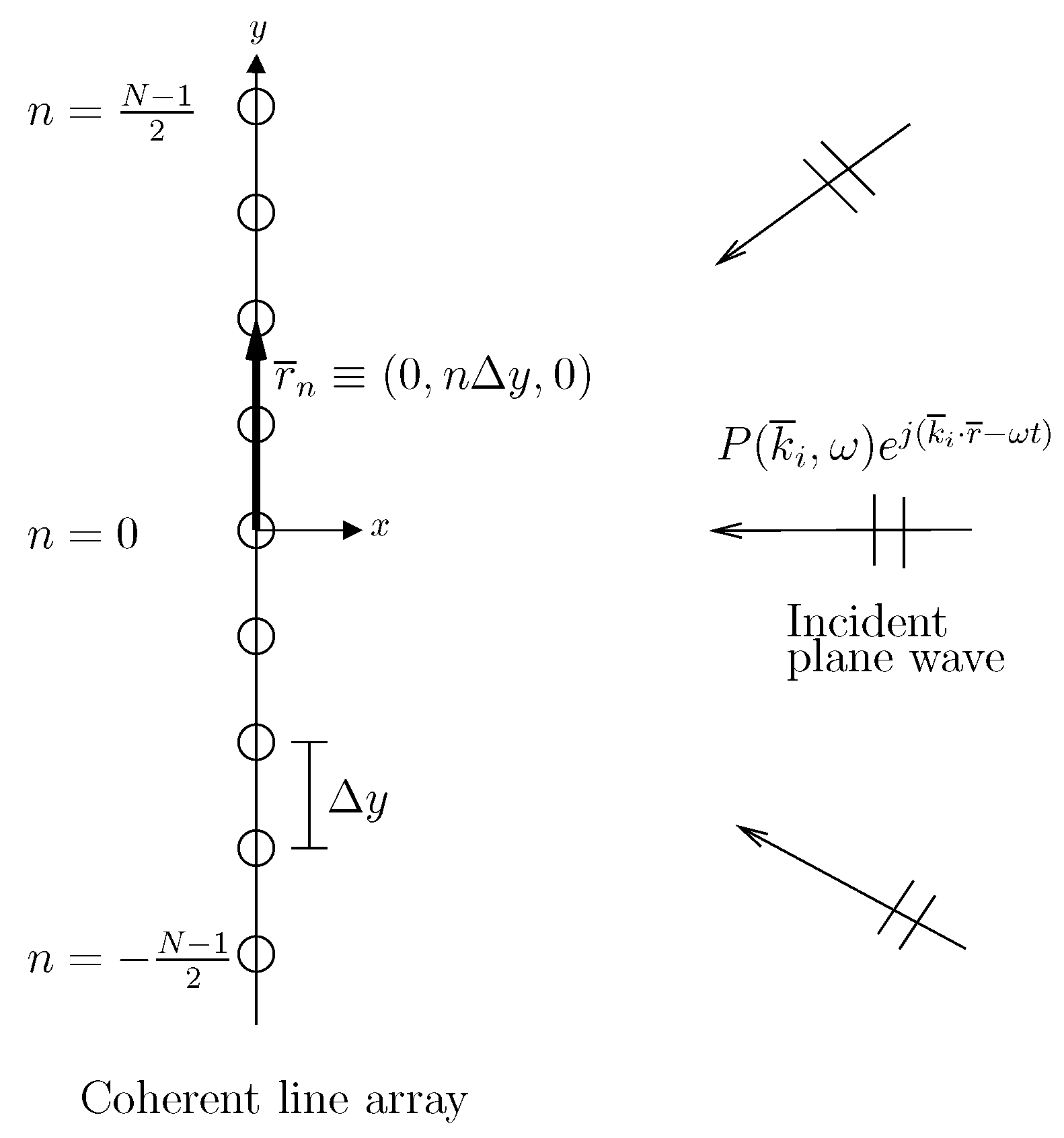
2.1. Beamformed Intensity Measurement on a Receiver Array

Let P i ( r ¯ , t ) = P ( k ¯ i , ω ) e j ( k ¯ i · r ¯ - ω t ) denote the pressure field at point r ¯ and time t due to a time-harmonic plane wave propagating in the direction of the acoustic wavenumber vector k ¯ i = k x i i ^ x + k y i i ^ y + k z i i ^ z , where P ( k ¯ i , ω ) is the complex plane wave amplitude, k = | k ¯ i | = ω / c is the acoustic wavenumber, ω is the radial frequency, c is the speed of sound and i is an index for i = 1 , 2 , 3 , . . . , M directions. A plane wave from any of these directions is incident on a discrete receiver array of length L containing N elements. The pressure field from any direction received on the n-th element of the array located at r ¯ n = ( 0 , y n , 0 ) (Figure 1) is P i ( r ¯ n , t ) = P ( k ¯ i , ω ) e j ( k y i y n - ω t ) .
The y-component of the wavenumber vector can be expressed as a function of the vertical inclination angle ψ and horizontal azimuthal angle θ of the incident plane wave as k y i = k sin ψ i sin θ i . Then, in the presence of M incident plane waves, assuming the inclination angle ψ i = π / 2 , the total pressure field received on the n-th element of the receiver array is:
P ( r ¯ n , t ) = i = 1 M P ( k ¯ i , ω ) e j ( k y n sin θ i - ω t )
The total beamformed pressure field at scan angle θ in terms of plane wave incident angle θ i is:
P B ( θ , t , ω ) = i = 1 M n = - N - 1 2 N - 1 2 P ( k ¯ i , ω ) e j ( k y n [ sin θ i - sin θ ] - ω t ) (2) = i = 1 M P ( k ¯ i , ω ) B ( sin θ - sin θ i , ω ) e - j ω t
where B ( sin θ , ω ) is the discrete array beam pattern given [1,2,3] by B ( sin θ , ω ) = 1 N sin k 2 N Δ y sin θ sin k 2 Δ y sin θ for θ spanning [ - π , 2 , π / 2 ] and array element spacing Δ y = L N - 1 .
The beamformed pressure field in Equation (2) is the convolution of the complex pressure amplitude of incident plane waves from different directions and the receiver array beam pattern. In the case of a single incident plane wave from direction θ 0 , Equation (2) simplifies to P B ( θ , t , ω ) = P ( k ¯ 0 , ω ) B ( sin θ - sin θ 0 , ω ) e - j ω t , which is proportional to the beam pattern steered in the direction of the incident plane wave, as illustrated in Figure A1 for a single incident plane wave at 30 .
The beamformed plane wave intensity measured on the array is then:
W ( θ , ω ) = | P B ( θ , t , ω ) | 2 = | i = 1 M P ( k ¯ i , ω ) B ( sin θ - sin θ i , ω ) | 2
By the central limit theorem, the incident plane wave complex amplitude P ( k ¯ i , ω ) follows circular complex Gaussian random (CCGR) statistics with zero mean due to random fluctuations arising from waveguide propagation, scattering, source mechanisms or a combination of these [4,5,6,11,12,13,14], such that P ( k ¯ i , ω ) = 0 . Moreover, incident plane wave fields from different directions are assumed to be independent of each other as found in typical OAWRS applications [4,5,6,13,14], such that P ( k ¯ i , ω ) P * ( k ¯ j , ω ) = P ( k ¯ i , ω ) P * ( k ¯ j , ω ) for i j . The expected beamformed intensity is then given by:
σ ( θ , ω ) = W ( θ , ω ) = i = 1 M S ( k ¯ i , ω ) | B ( sin θ - sin θ i , ω ) | 2
where S ( k ¯ i , ω ) = | P ( k ¯ i , ω ) | 2 is the expected intensity of the incident plane wave propagating in the direction k ¯ i .

2.2. Deconvolution of Beamformed Intensity from a Line Array: Maximum Likelihood Estimate of Expected Source Intensity

Beamformed intensity measurements (Equation (3)) at j = 1 , 2 , 3 , . . . , J discrete scan angles can be expressed as:
W j = W ( θ j , ω ) = | i = 1 M P ( k ¯ i , ω ) B ( sin θ j - sin θ i , ω ) | 2
which, in matrix form, can be written as:
W j = | i = 1 M P i B i j | 2
where P i = P ( k ¯ i , ω ) are the elements of a vector P and B i j = B ( sin θ j - sin θ i , ω ) are the elements of the scanning matrix B . The expected beamformed intensity from Equation (4) then becomes:
σ T = S T B
where the vector σ contains expected beamformed intensities W j , the vector S contains the expected plane wave intensities S i = S ( k ¯ i , ω ) = P ( k ¯ i , ω ) P * ( k ¯ i , ω ) from all horizontal azimuths and the elements of matrix B are B i j = | B i j | 2 .
The expected values of measurements W j = σ j ( S ) depend on the expected incident plane wave intensity vector S , which in general varies in space, and is to be estimated from W . In typical operational scenarios for OAWRS imaging, the combination of a sufficiently large, densely-sampled and spatially-tapered aperture [4,5,6,7] leads to low enough side lobes that non-overlapping beams are effectively independent for far field signal and noise sources. The conditional probability distribution for all measurements in vector W given S is then the product of gamma distributions [9,15]:
P ( W | S ) = j = 1 J μ j σ j ( S ) μ j W j μ j - 1 exp - μ j W j σ j ( S ) Γ ( μ j )
where μ j is the number of coherence cells in the intensity average derived from a sum of independent measurements, which is also equal to the signal-to-noise ratio W j 2 / ( W j 2 - W j 2 ) [9,15].
The log-transformed vector L defined by L j = ln ( W j / I r e f ) , where I r e f is the reference intensity, obeys the conditional distribution [15]:
P ( L | S ) = j = 1 J μ j σ j ( S ) μ j exp - μ j exp ( L j ) σ j ( S ) + μ j L j Γ ( μ j )
which is also the likelihood function, where σ j ( S ) = σ j ( S ) / I r e f . The log-likelihood function is then:
ln P ( L | S ) = j = 1 J μ j ln μ j σ j ( S ) + - μ j exp ( L j ) σ j ( S ) + μ j L j - ln Γ ( μ j )
The value of S for which the log-likelihood function attains its global maxima is the maximum likelihood estimate (MLE) of S ,
S ^ = arg max S ln P ( L | S )
which is also the value of S ^ for which the derivative of ln P ( L | S ) with respect to S vanishes:
d ln P ( L | S ) d S = j = 1 J - μ j σ j ( S ) d σ j ( S ) d S + μ j σ j ( S ) 2 W j I r e f d σ j ( S ) d S = 0 | S = S ^
The MLE of S is then:
S ^ = B d ^ σ B T - 1 B d ^ σ W
where the elements of diagonal matrix d ^ σ are d ^ σ j i = δ j i μ j / W j 2 and W j = W j / I r e f , as shown in Appendix A.2.
When the number of scan angles J is equal to the number of incident plane wave directions M, then matrices B and d ^ σ are square matrices, and Equation (13) simplifies to:
S ^ = B T - 1 W
and the solution of S ^ is linear in W .

2.3. Statistics of the Maximum Likelihood Estimator

A criterion to determine the performance of an estimator S ^ obtained from measurement vectors W or L is the Cramer–Rao Lower Bound (CRLB) on the parameter’s variance [22,23] given by:
Var ( S ^ i ) [ I - 1 ( ( S ) ) ] i i
where S i is the true parameter value and I ( S ) is the Fisher information matrix with elements:
[ I ] i n ( S ) = - 2 S i S n ln P ( L | S )
The Fisher information matrices for W and L are identical and equal to [11,15]:
[ I ] i n ( S ) = j = 1 J μ j σ j ( S ) 2 σ j ( S ) S i σ j ( S ) S n
which can be further simplified using Equation (7) to:
[ I ] i n ( S ) = j = 1 N μ j σ j ( S ) 2 B i j B n j I = B Ξ B T
where Ξ is a diagonal matrix with elements Ξ j j = μ j σ j ( S ) 2 .
In the case of M = J , Var ( S ^ i ) can be obtained from Equation (14) as:
Var ( S ^ i ) = Var ( B T - 1 W ) = j = 1 M B i j 2 σ j ( S ) 2 μ j (19) = Diagonal ( B Ξ - 1 B T )
where the matrix B = B T - 1 and Var ( W j ) = σ j ( S ) 2 μ j from the Gamma distribution of W j in Equation (8). The variance of the MLE when J = M then attains the CRLB, since it equals the diagonal elements of the inverse of I from Equation (18):
I - 1 = B T - 1 Ξ - 1 B - 1 (20) = B Ξ - 1 B T
For sufficiently large μ, the ML estimator’s probability distribution S ^ is asymptotically Gaussian given by [22,23]:
S ^ a N ( S , J - 1 ( S ) )
where the variance is asymptotically equal to the CRLB given in Equation (15), and the mean converges to the true parameter value making the ML estimator asymptotically optimal since it becomes unbiased and attains minimum variance [22,23].

3. Results: Illustrative Examples

Here, we use the maximum likelihood method to estimate the angular intensity distribution of incident plane waves from coherent line array measurements with analytic, synthetic and actual wide-area OAWRS imagery data [4,5,6]. In all of the examples shown in this section, N = 64 array elements spaced 0 . 75 m apart are used at a frequency of 950 Hz, as is consistent with some typical OAWRS imaging scenarios [4,5]. The array element spacing corresponds to half the acoustic wavelength for a cutoff frequency of 1000 Hz and speed of sound in water c = 1500 m/s.

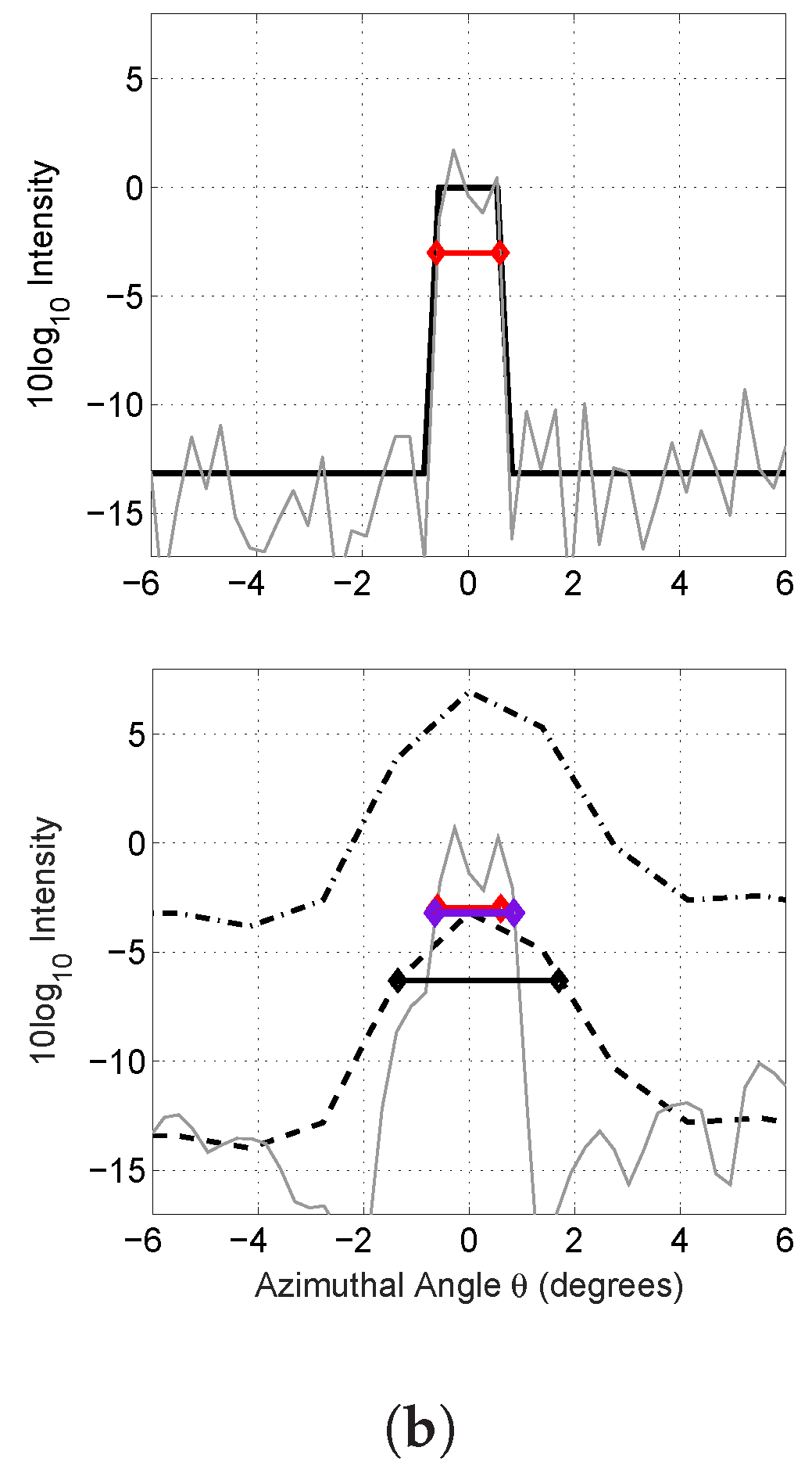
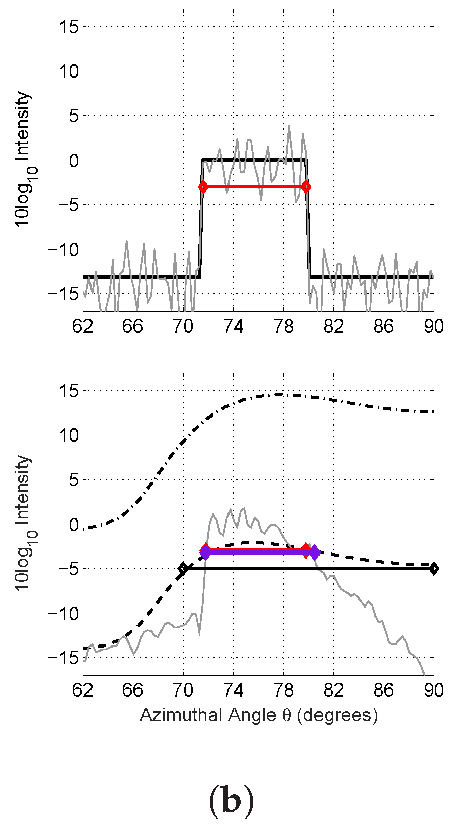
3.1. Analytic Solutions
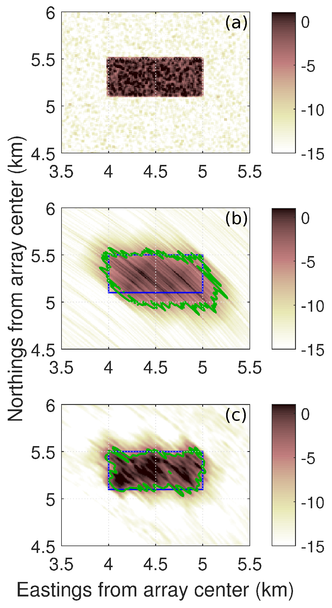
For a single incident plane wave with no signal dependent noise, the ML deconvolution of the conventional beamformed measurement results in the ground truth incident plane wave by invariance of the ML estimator [22,23], as illustrated for both broadside and end-fire incidence examples in Figure 2. This can be seen by noting that in the absence of randomness, the beamformed measurement is its expected value W = σ . The ML estimate can be then found analytically either via Equation (14) or via Equation (7), where resulting ML estimate S ^ becomes S , which is unity in the direction of the plane wave and zero elsewhere. Reversing the process, the convolution of this pressure field with the receiver array beam pattern yields the conventional beamformed data, which is the beam pattern itself shifted to the direction of the incident pressure field.

3.2. Synthetic Data

We now illustrate ML deconvolution of angular or spatial features sensed by nonuniform distributions of incident CCGR fields with synthetic data and numerical simulation (Figure 3, Figure 4 and Figure 5).
For prominent and relatively narrow angular box-like features, a roughly 50% improvement in angular resolution is found (Figure 3 and Figure 4). For a box-like feature of roughly 1 width at broadside, the 3-dB beamwidth of the deconvolved plane wave intensity distribution is found to be roughly 1.2 (Figure 3). This is roughly two times smaller than that from conventional beamforming of roughly 3 . Similarly, near array end-fire for a box-like feature of roughly an 8 width, the 3-dB beamwidth of the deconvolved plane wave intensity distribution is roughly 9 (Figure 4), which is roughly two-times smaller than the 20 width found in conventional beamforming. Only at much lower values at least 5–7 dB down from the peak intensity does the match between ground truth and ML deconvolved estimate deteriorate. This deterioration, however, is barely perceivable in a linear intensity scale. The expected intensity of the ML deconvolved estimate matches the ground truth well, within roughly ±1 dB for the broadside case and ±0.5 dB for the end-fire case. This comprises roughly an order of magnitude improvement over conventional beamforming, as shown in Figure 3 and Figure 4. In Figure 3 and Figure 4, a spatial Hanning window taper is applied; beamformed intensity is averaged over five independent and instantaneous realizations, such that μ = 5 for each W ( θ j , ω ) , as is consistent with typical OAWRS imaging [4,5]; simulations are performed as described in Appendix A.4; and the beamformed data W ( θ j , ω ) is deconvolved using the algorithm in Appendix A.5.
For a prominent and relatively wide two-dimensional box-like feature that extends both in azimuth and range from the receiver array center, a roughly 40% improvement in angular resolution over conventional beamforming is found (Figure 5). Such features are representative of actual fish distributions in the ocean [4,5,6]. The improvement in angular resolution is measured in terms of the spatial span or the area within the 3-dB down contour from the peak intensity of the feature after conventional beamforming and subsequent ML deconvolution with respect to the true areal coverage of the feature. For a feature centered at 50 from an array broadside of roughly a 9 width and a 1-km extent in range, the error in the spatial span of the ML deconvolved feature is roughly 8% of the true feature area. In comparison, the error in the spatial span of the feature from conventional beamforming is several times higher at roughly 50% of the true feature area. In Figure 5, a spatial Hanning window taper is applied; beamformed intensity is averaged over 10 independent and instantaneous realizations, such that μ = 5 for each W ( θ j , ω ) , as is consistent with typical OAWRS imaging [4,5]; simulations are performed as described in Appendix A.4; and the beamformed data W ( θ j , ω ) are deconvolved using the algorithm in Appendix A.5.

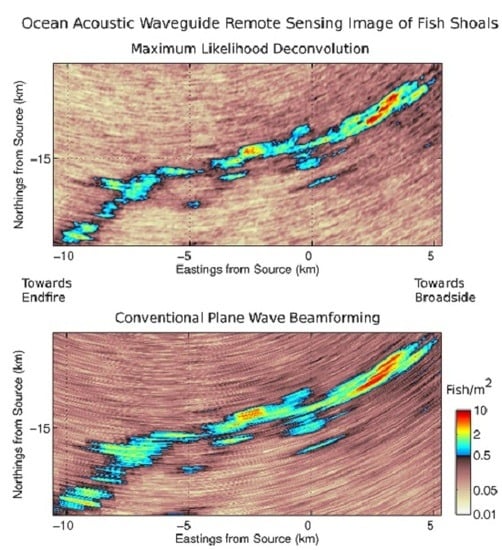
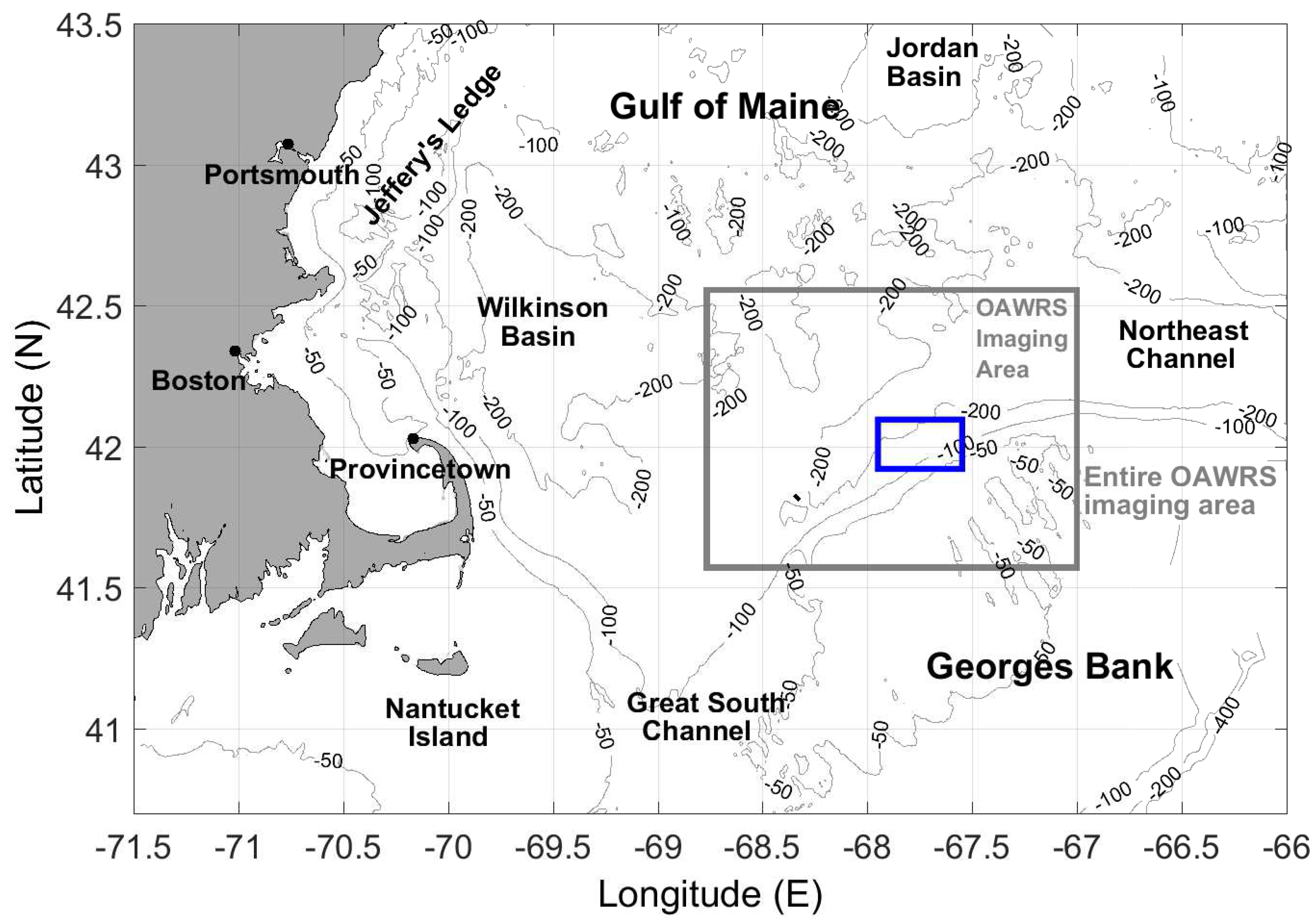
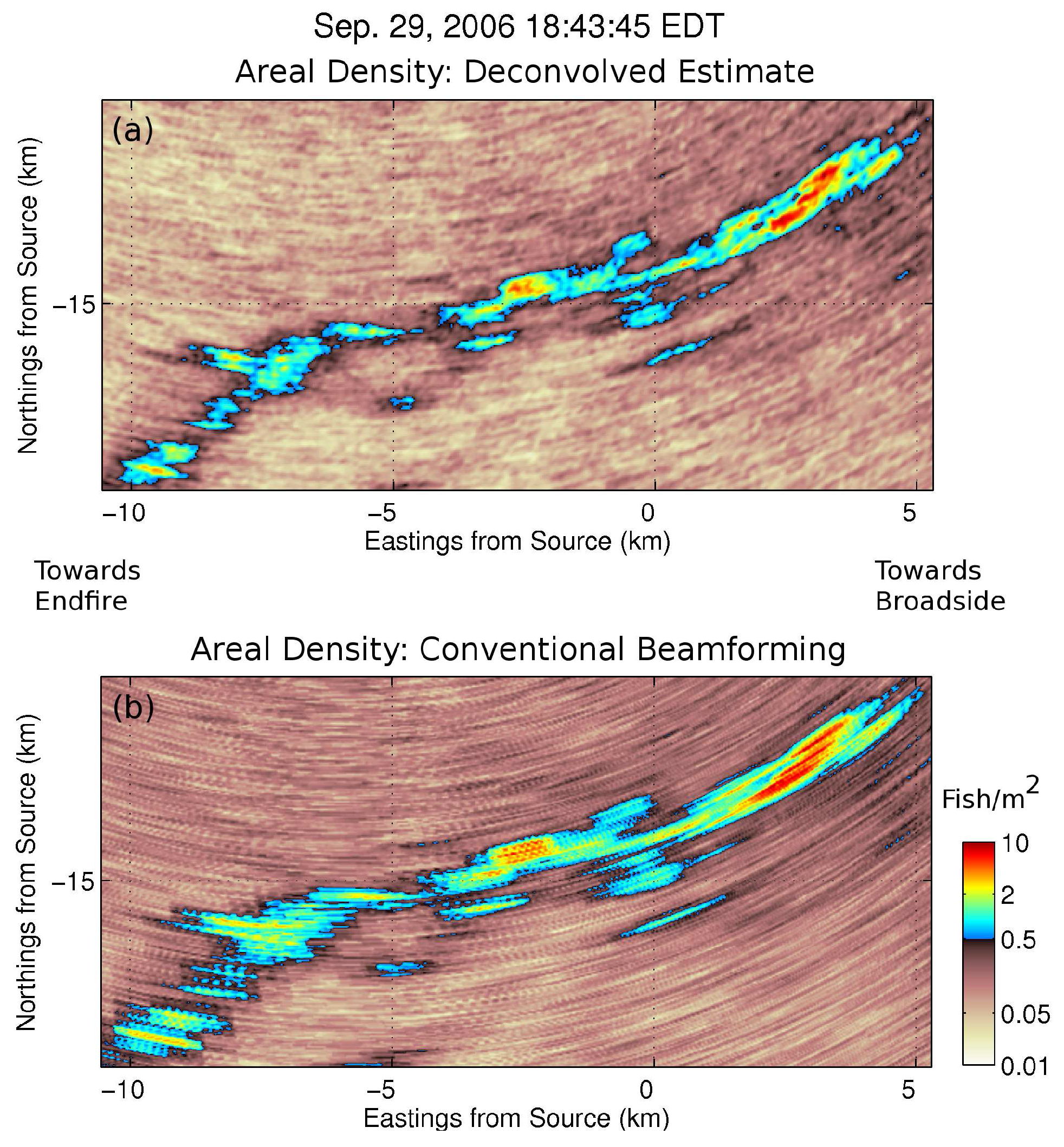
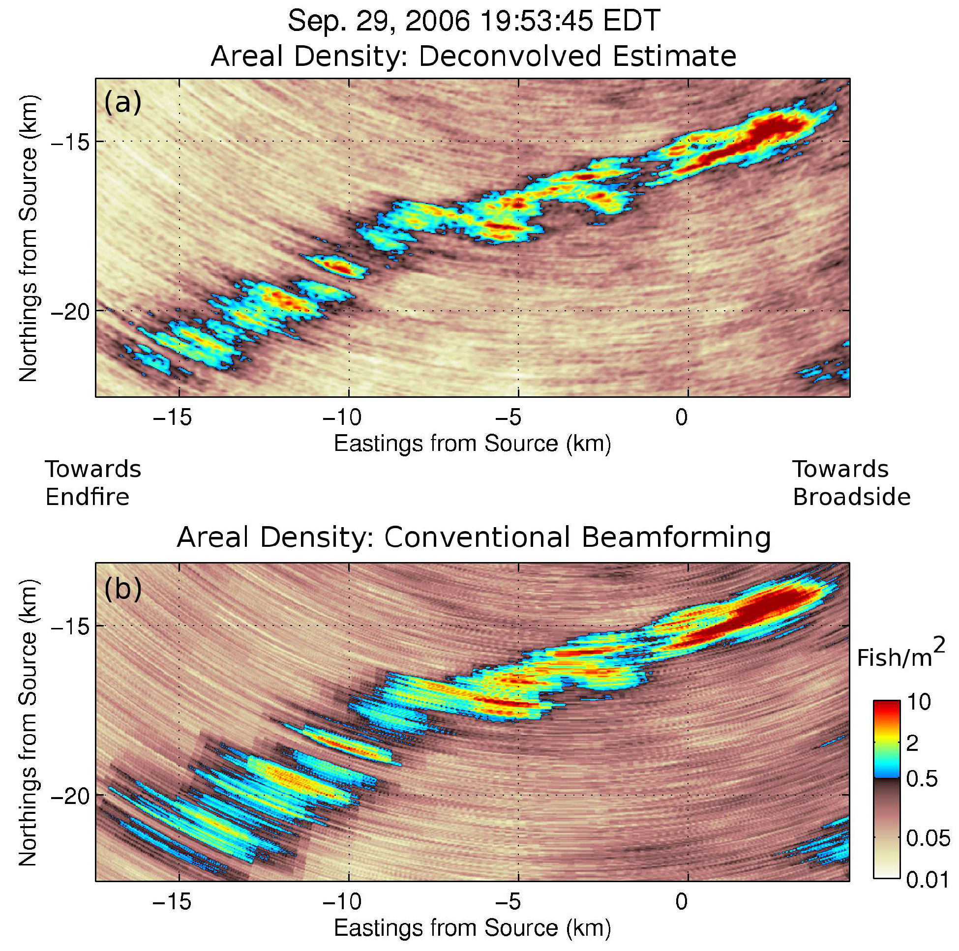
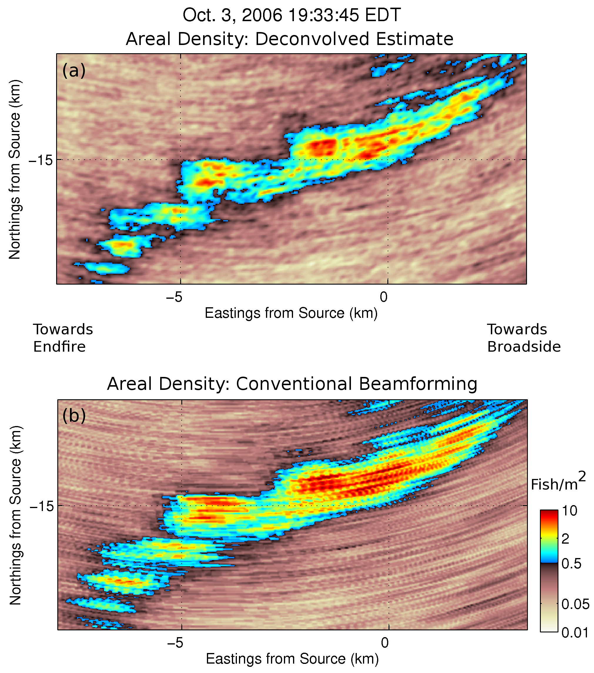
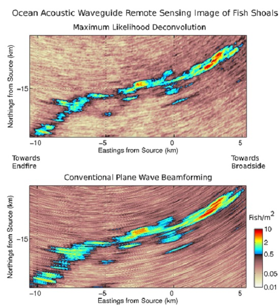
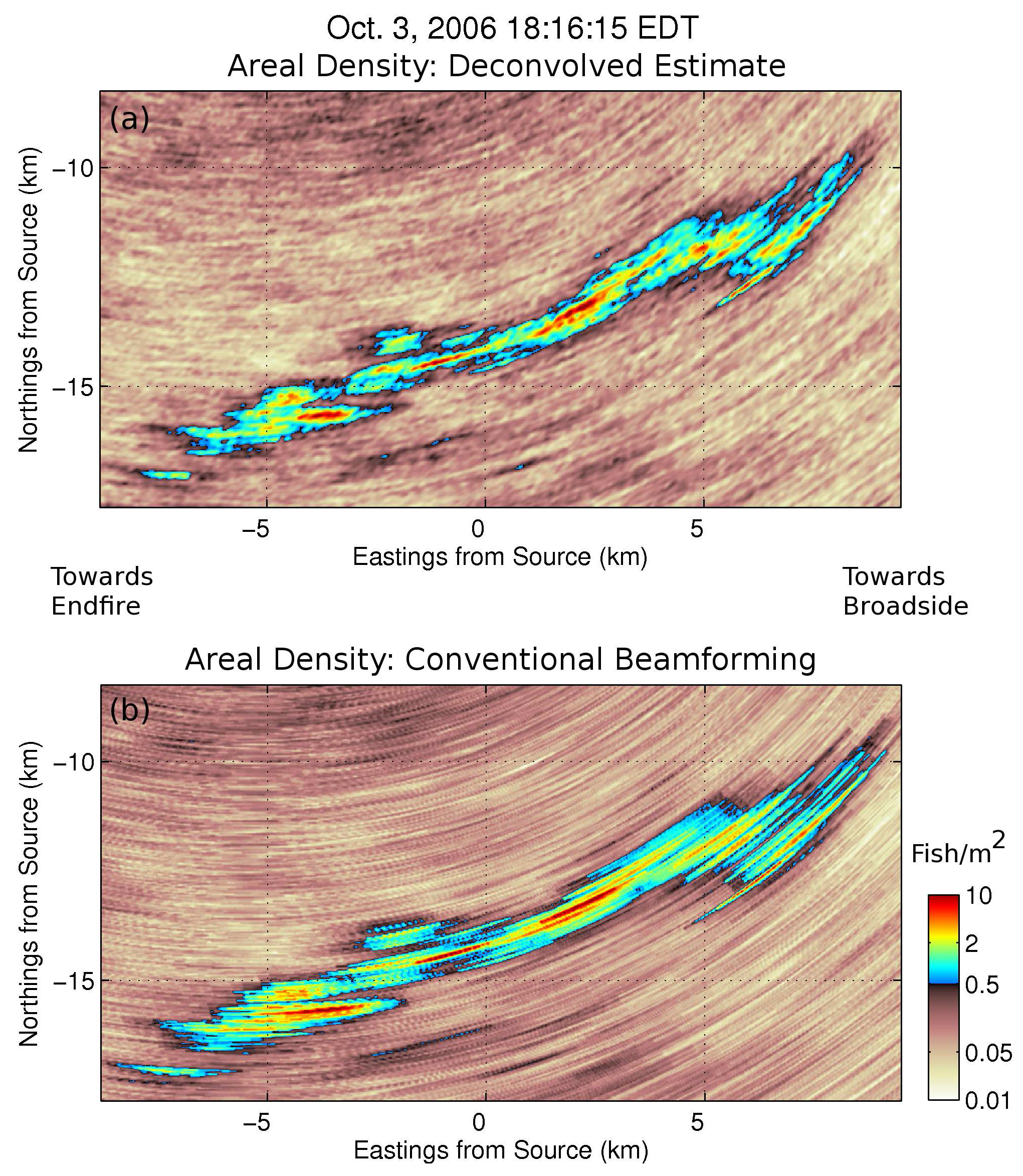
3.3. Ocean Acoustic Waveguide Remote Sensing Images of Fish Shoals

In the fall of 2006, vast shoals of spawning Atlantic herring were imaged using OAWRS in the Gulf of Maine (Figure 6) [5,6]. During evening hours, small clusters or schools of fish aggregated together to form large shoals spanning several tens of kilometers in length.
Maximum likelihood deconvolution of OAWRS fish shoal imagery leads to a roughly 10%–50% improvement in angular resolution over conventional beamforming (Figure 7, Figure 8, Figure 9 and Figure 10). For features located 20–50 from the array end-fire with population density >0.5 fish/m 2 (Figure 7, Figure 8, Figure 9 and Figure 10), a 40%–50% improvement in resolution is found. Similarly, for features located close to the array broadside, a 10%–25% improvement in resolution is found. The results indicate that ML improvements in angular resolution over conventional beamforming depend strongly on array beamwidth and the actual angular extent of the features. These results are consistent with synthetic data deconvolution results shown in Figure 3, Figure 4 and Figure 5.
In the OAWRS images shown in this section, N = 64 receiver array elements are spaced 0.75 m apart; the sensing frequency is 950 Hz; and a spatial Hanning window taper is applied to the receiver array elements [4,5]. The array element spacing corresponds to half the acoustic wavelength for a cutoff frequency of 1000 Hz and c = 1500 m/s. The OAWRS beamformed measurements are deconvolved using the algorithm in Appendix A.5.

4. Discussion

Following experimental observations from OAWRS measurements, we assume the demodulated field of incident plane waves from a discrete set of directions follows circular complex Gaussian random statistics (CCGR) arising from random wave propagation, scattering or radiation via the central limit theorem [4,5,6,11,12,13,14]. Intensity measurements then have signal-dependent noise. By time-harmonic plane-wave beamforming [2,3,22], the received intensity at the array center from different scan directions is determined and obeys a Gamma distribution [15,24]. Such standard plane-wave beamforming by Fourier transform from the spatial to the wavenumber domain, however, can non-linearly blur the angular distribution of incident plane waves for array geometries that lack spherical symmetry due to the nonlinear relationship between the incident direction and wavenumber components along the array caused by foreshortening.
By employing a sufficiently large aperture and applying a spatial taper function across the array as in OAWRS applications, distinct directional beams are effectively statistically independent [4,5,6,7] for the far field signals and noise sources typically encountered in OAWRS. Maximizing the likelihood function for these independent beams then yields the maximum likelihood estimate of intensity incident from a given parameterized angular sector, which acts as a deconvolution process to extract the angular distribution of the incident planewave field from blurring caused by the array’s diffraction limited beam pattern.
The far field signal and noise sources encountered in OAWRS typically have correlation along the array [4,5,6,13,14] that is not known a priori. Past statistical models for acoustic beamforming, including past maximum likelihood approaches, in the ocean are not well suited to OAWRS applications, because they have overwhelmingly assumed a deterministic signal model in additive Gaussian noise with a priori knowledge of the noise’s spatial correlation, which is most often assumed to be spatially uncorrelated for horizontal apertures’ element spacing exceeding half the wavelength [16,17,18,19,20,21]. Neither of these assumptions is consistent with those observed in OAWRS sensing, where both signal and noise fields are random and highly correlated in space across the array due to their far field origins. Additionally, it has been noted [25] that some persistent confusion and misidentification has occurred between maximum likelihood [22,23] and other methods [19,20,21] in beamforming applications.

5. Conclusions

A maximum likelihood method is developed to deconvolve underwater acoustic intensity images corrupted with signal-dependent noise. The images are assumed to be generated by planewave beamforming of data received from a coherent spatial receiving array. The method is shown to enable significant improvements in resolving the directions of incident plane waves over conventional planewave beamforming by theoretical analysis, numerical simulation and the application to experimental data. Deconvolution of experimentally-measured Ocean Acoustic Waveguide Remote Sensing (OAWRS) images of fish areal population density show an angular resolution improvement of 40%–50% for fish clusters close to the array end-fire and 10%–25% for fish clusters close to the array broadside. The approach developed is generally applicable to planewave beamforming on multidimensional arrays of arbitrary geometry. Line array implementations are presented here for simplicity and to provide examples relevant to typical OAWRS scenarios.
multiple

Acknowledgments

This research was supported by the Office of Naval Research and the National Oceanographic Partnership Program.

Author Contributions

Ankita D. Jain and Nicholas C. Makris developed the approach, analyzed the data, and wrote the paper.

Conflicts of Interest

The authors declare no conflict of interest.

Appendix A.

Appendix A.1 Beamformed Pressure Field for a Single Plane Wave

The beamformed pressure field P B ( θ , t , ω ) (Equation (2)) for a single plane wave is proportional to the beam pattern steered in the direction of the plane wave and depends on the number of sensors N, element spacing Δ y and incident wavenumber k = 2 π f c , where f is the sensing frequency and c the speed of sound. Figure A1 shows the beamformed pressure field due to a single plane wave incident from 30 from broadside for a typical OAWRS mid-frequency aperture configuration for a range of sensing frequencies where N = 64 , Δ y = 1 2 c f 0 for a cutoff frequency f 0 = 1000 Hz [4,5]. The main lobe width is narrowest and, so, has the best angular resolution when the sensing frequency equals the cutoff frequency of 1000 Hz. As the sensing frequency decreases and the aperture remains the same, the angular resolution becomes proportionally worse.
Figure A1. Beamformed pressure field P B ( θ , t , ω ) due to a single plane wave of unit amplitude incident from a direction 30 from broadside measured on a discrete line array as shown in Figure 1 for various plane wave frequencies. Here, the array contains N = 64 elements and Δ y = 1 2 c f 0 , where the array cutoff frequency f 0 = 1000 Hz and speed of sound c = 1500 m/s.
Remotesensing 08 00694 g011

Appendix A.2 Derivation of the Matrix form of MLE of Deconvolved Plane Wave Intensity

From Equation (7), the derivative of the expected beamformed intensity vector normalized with respect to I r e f is given by:
d σ j ( S ) d S i = | B i j | 2 / I r e f = B i j / I r e f
Then, Equation (12) can be written in vector form as:
j = 1 J B i j μ j σ j ( S ) | S = S ^ = j = 1 J B i j μ j W j σ j ( S ) 2 | S = S ^
or:
B d σ σ ( S ) | S = S ^ = B d σ W | S = S ^
where W = W / I r e f and d σ j i = δ j i μ j / σ j ( S ) 2 are the elements of a diagonal matrix. By inserting Equations (7) into (A3) and given d σ , the MLE of S is:
S ^ = B d σ B T - 1 B d σ W
Typically, d σ is not known a priori and, so, needs to be estimated. If the MLE of σ j ( S ) is W j , then by the invariance of the MLE, d ^ σ is the MLE of d σ with elements d ^ σ j i = δ j i μ j / W j 2 . The MLE of S is then:
S ^ = B d ^ σ B T - 1 B d ^ σ W

Appendix A.3 A Conventional Beamformer Normalization Useful for Continuous and Relatively Uniform Incident Plane-Wave Distributions

A uniform distribution of incident plane waves P ( θ i , ω ) results in scan-angle θ j -dependent conventional beamformed intensities W ( θ j , ω ) , as shown in Figure A2, due to the nonuniform angular resolution across scan angles caused by foreshortening. This is because of the convolution of the uniformly-spaced incident plane wave pressure field with a beam pattern that has a narrower beamwidth at the array broadside and wider beamwidth at the array end-fire in the θ domain.
Figure A2. A comparison between incident plane wave intensity distribution, the corresponding conventional beamforming and the beamforming with a scan-angle-dependent normalization (Equation (A6)) applied to it.
Remotesensing 08 00694 g012
A scan-angle-dependent intensity normalization:
I norm , j = I norm ( θ j ) = i = 1 M | B ( sin θ j - sin θ i ) | 2
is applied to conventional beamformed measurement, such that W norm ( θ j , ω ) = W j / I norm , j . The effect of this normalized beam pattern is shown in Figure 3 and Figure 4. This normalization is also applied in Figure 5.

Appendix A.4 Numerical Simulation of Synthetic Beamformed Data

For the synthetic data deconvolution results presented in Section 3.2, a ground truth incident plane wave distribution P ( k ¯ i , ω ) for i = 1 , 2 , 3 . . . M incident angles is convolved with the array beam pattern B ( sin θ , ω ) to yield the synthetic beamformed pressure field P B ( θ , t , ω ) given in Equation (2). The beamformed plane wave intensity W ( θ , ω ) and its expected value σ ( θ , ω ) are then determined using Equations (3) and (4), respectively. Maximum likelihood deconvolution of the expected plane wave intensity distribution S ( k ¯ i , ω ) is then performed using the approach outlined in Appendix A.5.

Appendix A.5 Numerical Implementation of the Deconvolution Algorithm

An iterative scheme involving steepest descent and simulated annealing [26] is used to determine the deconvolved source distribution estimate S ^ from beamformed data W .
Step 1.
The beamformed intensity vector is given by W ( θ j , ω ) for j = 1 , 2 , . . . , J scanning directions. Select starting solution vectors:
P start = P 0 (A7) S start = S 0 = | P 0 | 2
for pressure field and intensity vectors, respectively, of length M for M azimuthal directions. A CCGR field with variance equal to the background signal-independent noise intensity is a reasonable starting point for P .
Step 2.
Every iteration vector attempts to move the log-likelihood function in Equation (10) to its global maximum. Specifically, at the q-th iteration, determine the log likelihood function ln P ( L trial | S trial q ) for the trial solution matrix:
S trial q = ( P trial q ) 2
containing 2 M trial solutions. The matrix ( P trial q ) is of size M × 2 M where the rows represent a given trial solution vector for M azimuthal directions and columns represent 2 M trial solutions. Each trial solution contains a positive or negative increment to the trial solution of the ( q - 1 )-th iteration in only one azimuthal direction, which makes the 2 M increment vectors in the trial solutions orthogonal to each other. Specifically, the pressure field at the jth azimuthal direction of the ith trial solution is given by:
p trial , ( j , i ) q = p j , i q - 1 + ϵ α δ i j + β
and the corresponding intensity is given by:
S trial , ( j , i ) q = | p trial , ( j , i ) q | 2
where ϵ = 1 for i = 1 , 2 , . . . , M and ϵ = - 1 for i = M + 1 , M + 2 , . . . , 2 M , j = 1 , 2 , . . . , M for M azimuthal directions. At every step, a single trial solution is updated. Once all trial solutions are updated sequentially, that is the end of the q-th iteration. Here, δ i j is the Kronecker delta function and, so, takes the value of one if i = j and is zero otherwise, and α is the step size. To move a solution that is stuck in a local minimum, randomly generated noise β, which is drawn from CCGR distribution, is added at every iteration.
Step 3.
Find the i-th vector that maximizes the log-likelihood function:
i 0 = max i { ln P ( L | S trial , ( i = 1 : 2 M , j = 1 : M ) q ) }
The updated solution vector for the q-th iteration then is:
p j q = p trial , ( j , i 0 ) q
This is the end of the q-th iteration. Repeat Steps 2–3 until the value of the maximum likelihood function converges. The maximum likelihood estimate S ^ is the one for which ln P ( L | S ) is the maximum over all iterations. At this value, the estimated beamformed intensity also converges to W in the least square sense [22,23].
In all examples shown, a large number of azimuthal directions M, typically 5–9-times the number of scan angles J, is used to make the distribution approximately continuous in the azimuth.

References

  1. Urick, R.J. Principles of Underwater Sound; McGraw Hill: New York, NY, USA, 1983. [Google Scholar]
  2. Tolstoy, I.; Clay, C. Ocean Acoustics: Theory and Experiment in Underwater Sound; McGraw-Hill: New York, NY, USA, 1966. [Google Scholar]
  3. Van Trees, H.L. Detection, Estimation, and Modulation Theory, Part I; Wiley-Interscience: New York, NY, USA, 2001. [Google Scholar]
  4. Makris, N.C.; Ratilal, P.; Symonds, D.T.; Jagannathan, S.; Lee, S.; Nero, R.W. Fish population and behavior revealed by instantaneous continental shelf-scale imaging. Science 2006, 311, 660–663. [Google Scholar] [CrossRef] [PubMed]
  5. Makris, N.C.; Ratilal, P.; Jagannathan, S.; Gong, Z.; Andrews, M.; Bertsatos, I.; Godø, O.R.; Nero, R.W.; Jech, J.M. Critical population density triggers rapid formation of vast oceanic fish shoals. Science 2009, 323, 1734–1737. [Google Scholar] [CrossRef] [PubMed]
  6. Gong, Z.; Andrews, M.; Jagannathan, S.; Patel, R.; Jech, J.M.; Makris, N.C.; Ratilal, P. Low-frequency target strength and abundance of shoaling Atlantic herring (Clupea harengus) in the Gulf of Maine during the Ocean Acoustic Waveguide Remote Sensing 2006 Experiment. J. Acoust. Soc. Am. 2010, 127, 104–123. [Google Scholar] [CrossRef] [PubMed]
  7. Ratilal, P.; Lai, Y.; Symonds, D.T.; Ruhlmann, L.A.; Preston, J.R.; Scheer, E.K.; Garr, M.T.; Holland, C.W.; Goff, J.A.; Makris, N.C. Long range acoustic imaging of the continental shelf environment: The Acoustic Clutter Reconnaissance Experiment 2001. J. Acoust. Soc. Am. 2005, 117, 1977–1998. [Google Scholar] [CrossRef] [PubMed]
  8. Bergmann, P.G. The Physics of Sound in the Sea; Research Analysis Group: Wakefield, MA, USA, 1946. [Google Scholar]
  9. Goodman, J.W. Statistical Optics; Wiley-Interscience: New York, NY, USA, 1985. [Google Scholar]
  10. DiFranco, J.V.; Rubin, W.L. Radar Detection; Prentice-Hall: Englewood Cliffs, NJ, USA, 2004. [Google Scholar]
  11. Makris, N.C. The effect of saturated transmission scintillation on ocean acoustic intensity measurements. J. Acoust. Soc. Am. 1996, 100, 769–783. [Google Scholar] [CrossRef]
  12. Makris, N.C. Parameter resolution bounds that depend on sample size. J. Acoust. Soc. Am. 1996, 99, 2851–2861. [Google Scholar] [CrossRef]
  13. Jagannathan, S.; Küsel, E.T.; Ratilal, P.; Makris, N.C. Scattering from extended targets in range-dependent fluctuating ocean-waveguides with clutter from theory and experiments. J. Acoust. Soc. Am. 2012, 132, 680–693. [Google Scholar] [CrossRef] [PubMed]
  14. Tran, D.; Andrews, M.; Ratilal, P. Probability distribution for energy of saturated broadband ocean acoustic transmission: Results from Gulf of Maine 2006 experiment. J. Acoust. Soc. Am. 2012, 132, 3659–3672. [Google Scholar] [CrossRef] [PubMed]
  15. Makris, N.C. A foundation for logarithmic measures of fluctuating intensity in pattern recognition. Opt. Lett. 1995, 20, 2012–2014. [Google Scholar] [CrossRef] [PubMed]
  16. Hinich, M.J. Maximum-likelihood signal processing for a vertical array. J. Acoust. Soc. Am. 1973, 54, 499–503. [Google Scholar] [CrossRef]
  17. Zhang, C.; Florêncio, D.; Ba, D.E.; Zhang, Z. Maximum likelihood sound source localization and beamforming for directional microphone arrays in distributed meetings. IEEE Trans. Multimed. 2008, 10, 538–548. [Google Scholar] [CrossRef]
  18. Baggeroer, A.B.; Kuperman, W.A.; Mikhalevsky, P.N. An overview of matched field methods in ocean acoustics. IEEE J. Ocean. Eng. 1993, 18. [Google Scholar] [CrossRef]
  19. Johnson, D.H. The application of spectral estimation methods to bearing estimation problems. Proc. IEEE 1982, 70, 1018–1028. [Google Scholar] [CrossRef]
  20. Baggeroer, A.; Kuperman, W.; Schmidt, H. Matched field processing: Source localization in correlated noise as an optimum parameter estimation problem. J. Acoust. Soc. Am. 1988, 83, 571–587. [Google Scholar] [CrossRef]
  21. Kuperman, W.A.; Collins, M.D.; Perkins, J.S.; Davis, N. Optimal time-domain beamforming with simulated annealing including application of apriori information. J. Acoust. Soc. Am. 1990, 88, 1802–1810. [Google Scholar] [CrossRef]
  22. Kay, S.M. Fundamentals of Statistical Signal Processing, Volumes I and II; Pearson Education: Upper Saddle River, NJ, USA, 1998. [Google Scholar]
  23. Rao, C.R. Linear Statistical Inference and Its Applications; John Wiley & Sons: New York, NY, USA, 2009. [Google Scholar]
  24. Goodman, J.W. Statistical Optics; Wiley: New York, NY, USA, 1985. [Google Scholar]
  25. Haykin, S. Advances in Spectrum Analysis and Array Processing (Vol. III); Prentice-Hall, Inc.: Englewood Cliffs, NJ, USA, 1995. [Google Scholar]
  26. Kelley, C.T. Iterative Methods for Optimization; SIAM: Philadelphia, PA, USA, 1999. [Google Scholar]
Figure 1. A sketch of the array geometry and incident plane wave field.
Remotesensing 08 00694 g001
Figure 2. A comparison between ground truth expected plane wave intensity S ( k ¯ i , ω ) , conventional beamforming W ( θ j , ω ) and beamforming using ML deconvolution S ^ ( k ¯ i , ω ) using an array with a rectangular taper for synthetically-generated plane waves in the limit of no signal-dependent noise incident at (a) array broadside and (b) array endfire. The ML deconvolution estimate can be determined analytically by inspection of Equation (14) in the absence of noise for a single incident plane wave.
Remotesensing 08 00694 g002
Figure 3. For a narrow feature at broadside, (a) a comparison between ground truth expected plane wave intensity S ( k ¯ i , ω ) , plane wave intensity with signal dependent noise averaged over five realizations, conventional beamforming W ( ω , θ j ) , conventional beamforming with normalization (Appendix A.3) and beamforming using ML deconvolution S ^ ( k ¯ i , ω ) for synthetically-generated plane waves with signal-dependent noise spanning all scan angles with signal dependent noise; (b) a zoomed in version of (a) within the highlighted box shown. The horizontal bars in (b) represent the 3-dB down widths from the peak expected value of the true intensity distribution (red), the ML deconvolved intensity estimate (blue) and the conventional beamforming intensity measurement (black).
Remotesensing 08 00694 g003aRemotesensing 08 00694 g003b
Figure 4. Same as Figure 3, except for a feature close to the array end-fire. (a) A comparison between ground truth expected plane wave intensity S ( k ¯ i , ω ) , plane wave intensity with signal dependent noise averaged over five realizations, conventional beamforming W ( ω , θ j ) , conventional beamforming with normalization (Appendix A.3) and beamforming using ML deconvolution S ^ ( k ¯ i , ω ) for synthetically-generated plane waves with signal-dependent noise; (b) a zoomed in version of (a) within the highlighted box shown.
Remotesensing 08 00694 g004aRemotesensing 08 00694 g004b
Figure 5. A comparison between the (a) ground truth plane wave intensity distribution, (b) conventional beamformed measurement normalized for scan-angle-dependent beamwidth variation (Appendix A.3) and (c) beamforming using ML deconvolution (bottom) for a synthetic two-dimensional plane wave intensity distribution. The color bar shows the logarithm of the plane wave intensity distribution in dB. In (b,c), the solid green curves represent the 3-dB down contour from the average intensity within the ground truth plane wave distribution, and the blue lines represent the true boundary of the plane wave intensity distribution. The receiver array is set to be positioned along the x-axis centered at the origin (0, 0).
Remotesensing 08 00694 g005
Figure 6. Gulf of Maine showing the OAWRS imaging area (gray box) and the more specific region corresponding to Figure 7, Figure 8, Figure 9, Figure 10 (blue box).
Remotesensing 08 00694 g006
Figure 7. Comparison of (a) ML deconvolved and (b) conventional beamformed areal population density of a large spawning Atlantic herring shoal measured on 29 September 2006 at 18:43 EDT, as shown in Figure 4b, of Makris et al. [5]. The beamformed intensity shown is averaged over six independent and instantaneous image realizations, such that μ = 6 for each pixel [5]. The measured conventional beamformer data W are deconvolved using the algorithm in Appendix A.5 and then converted to areal density maps as in Makris et al. [4,5].
Remotesensing 08 00694 g007
Figure 8. Same as Figure 7 showing a comparison of (a) ML deconvolved and (b) conventional beamformed areal population density of a herring shoal measured on 29 September 2006 at 19:53 EDT, as shown in Figure 4c of Makris et al. [5].
Remotesensing 08 00694 g008
Figure 9. Same as Figure 7 showing a comparison of (a) ML deconvolved and (b) conventional beamformed areal population density of a herring shoal measured on 3 October 2006 at 18:15 EDT, as shown in Figure 1g of Makris et al. [5].
Remotesensing 08 00694 g009
Figure 10. Same as Figure 7 showing a comparison of (a) ML deconvolved and (b) conventional beamformed areal population density of a herring shoal measured on 3 October 2006 at 19:33 EDT, as shown in Figure 1h of Makris et al. [5].
Remotesensing 08 00694 g010

