Abstract
Forest topsoil supports vegetation growth and contains the majority of soil nutrients that are important indices of soil fertility and quality. Therefore, estimating forest topsoil properties, such as soil organic matter (SOM), total nitrogen (Total N), pH, litter-organic (O-A) horizon depth (Depth) and available phosphorous (AvaP), is of particular importance for forest development and management. As an emerging technology, light detection and ranging (LiDAR) can capture the three-dimensional structure and intensity information of scanned objects, and can generate high resolution digital elevation models (DEM) using ground echoes. Moreover, great power for estimating forest topsoil properties is enclosed in the intensity information of ground echoes. However, the intensity has not been well explored for this purpose. In this study, we collected soil samples from 62 plots and the coincident airborne LiDAR data in a Korean pine forest in Northeast China, and assessed the effectiveness of both multi-scale intensity data and LiDAR-derived topographic factors for estimating forest topsoil properties. The results showed that LiDAR-derived variables could be robust predictors of four topsoil properties (SOM, Total N, pH, and Depth), with coefficients of determination (R2) ranging from 0.46 to 0.66. Ground-returned intensity was identified as the most effective predictor for three topsoil properties (SOM, Total N, and Depth) with R2 values of 0.17–0.64. Meanwhile, LiDAR-derived topographic factors, except elevation and sediment transport index, had weak explanatory power, with R2 no more than 0.10. These findings suggest that the LiDAR intensity of ground echoes is effective for estimating several topsoil properties in forests with complicated topography and dense canopy cover. Furthermore, combining intensity and multi-scale LiDAR-derived topographic factors, the prediction accuracies (R2) were enhanced by negligible amounts up to 0.40, relative to using intensity only for topsoil properties. Moreover, the prediction accuracy for Depth increased by 0.20, while for other topsoil properties, the prediction accuracies increased negligibly, when the scale dependency of soil–topography relationship was taken into consideration.
1. Introduction
Forest topsoil properties, such as soil organic matter (SOM), total nitrogen (Total N), pH, O-A horizon depth (Depth) and available phosphorous (AvaP), are the most important indices for soil fertility and quality [1]. Accurate estimation of topsoil properties is therefore essential for forest productivity, sustainable soil utilization, and management [2].
Estimation of forest topsoil properties over large areas is an important subject in soil science. Generally, estimating factors of forest topsoil properties using traditional methods can be categorized into two groups: based on topographic factors and based on soil spectral reflectance information [3]. DEM-derived topographic factors, including but not limited to elevation, slope, aspect, and topographic wetness, have been shown to be effective predictors of SOM, Total N, pH, Depth, hydraulic factors and other soil properties across different spatial scales. It is worth pointing out that the soil–topography relationship is often scale dependent, requiring multi-scale DEM-derived topographic factors for estimating topsoil properties. Furthermore, recent studies showed that the neighbor extent had affected soil–terrain correlations to a greater degree than grid resolution [4,5,6,7,8,9,10,11,12,13], and neighbor extent was worth considering. As for soil spectral reflection information, previous studies found that there was a strong correlation between certain soil properties (including soil total carbon, SOM, Total N, mineralized nitrogen, pH value, etc.) and soil spectral reflectance in the NIR-SWIR (near infrared to short wave infrared) range, with R2 values greater than 0.8 [9,10,11,12]. The radiation within NIR region is absorbed by various chemical bonds, such as C–H, C=O, N–H, and O–H present in soil samples. Furthermore, the radiation is proportionally absorbed with respect to the concentration of these compounds. As a result, the reflectance spectra of NIR essentially contain information about the organic composition of the soil [14,15,16,17]. Soil spectral reflectance therefore has also been adopted for estimating topsoil properties.
As an emerging active remote sensing technology, light detection and ranging (LiDAR) can provide high resolution three-dimensional (3D) information for target objects. In the past two decades, 3D spatial information has been widely applied in forest ecology, including but not limited to estimation of forest biomass, extraction of standing height and stem volume, distinguishing forest habitat types, and assessing biodiversity [18,19,20,21,22,23]. One of the most important LiDAR products is the high resolution topographic map interpolated from ground echoes. The LiDAR-derived high resolution digital elevation model (DEM) can be used to generate slope layer, aspect layer, topographic wetness index (WI), relative stream power index (RSP), sediment transport index (STI), total curvature (TC) and so on, and those DEM-derived products together with the DEM layer are powerful tools for estimating soil properties. Furthermore, LiDAR data can “penetrate” dense forest canopy even in mountainous areas, providing high resolution DEM information where traditional aerial photogrammetry- and optical sensor-derived DEM products remain highly uncertain [24,25,26,27].
In addition to 3D DEM information, LiDAR data also provide “intensity” information associated with each laser hit, which is strongly related to the spectral reflectance of targets [28,29,30,31]. Intensity information is a relative measure of the integration of power received over time for given return signals [32]. When spectral characteristics of target objects are different, their reflectance varies [33,34]. Because LiDAR intensity is a function of many factors, it has not been widely used in forest ecology, and what can be accomplished using LiDAR intensity information remains limited. To exclude the influence of factors such as weather, distance, and scale, normalization, filtering, distance calibration, resampling, and radiation calibration have been commonly adopted to calibrate intensity data. Using intensity information, previous studies focused on detecting inundated understory areas [35], lithological mapping [36], land cover classification [37,38,39], and estimating C stocks above- and below-ground in boreal forests [40]. In the area of soil sciences, intensity information has only been used to estimate soil properties like soil surface moisture [41,42], surface roughness [43], and texture [44].
Although LiDAR can provide two important variables: LiDAR-derived intensity of ground echoes and topographic factors. Few studies have used LiDAR-derived intensity of ground returns and multi-scale topographic factors to predict topsoil properties.
In the present study, we acquired small footprint airborne LiDAR data and data on soil properties in a Korean pine mixed forest in northeastern China, and explored the effectiveness of multi-scale LiDAR-derived intensity and topographic information for predicting soil properties. In detail, the objectives of our study were to explore: (1) whether forest topsoil properties can be estimated by multi-scale LiDAR-derived intensity and topographic factors; and (2) what accuracies can be achieved using LiDAR-derived factors to estimate forest topsoil properties.
2. Materials and Methods
2.1. Study Area
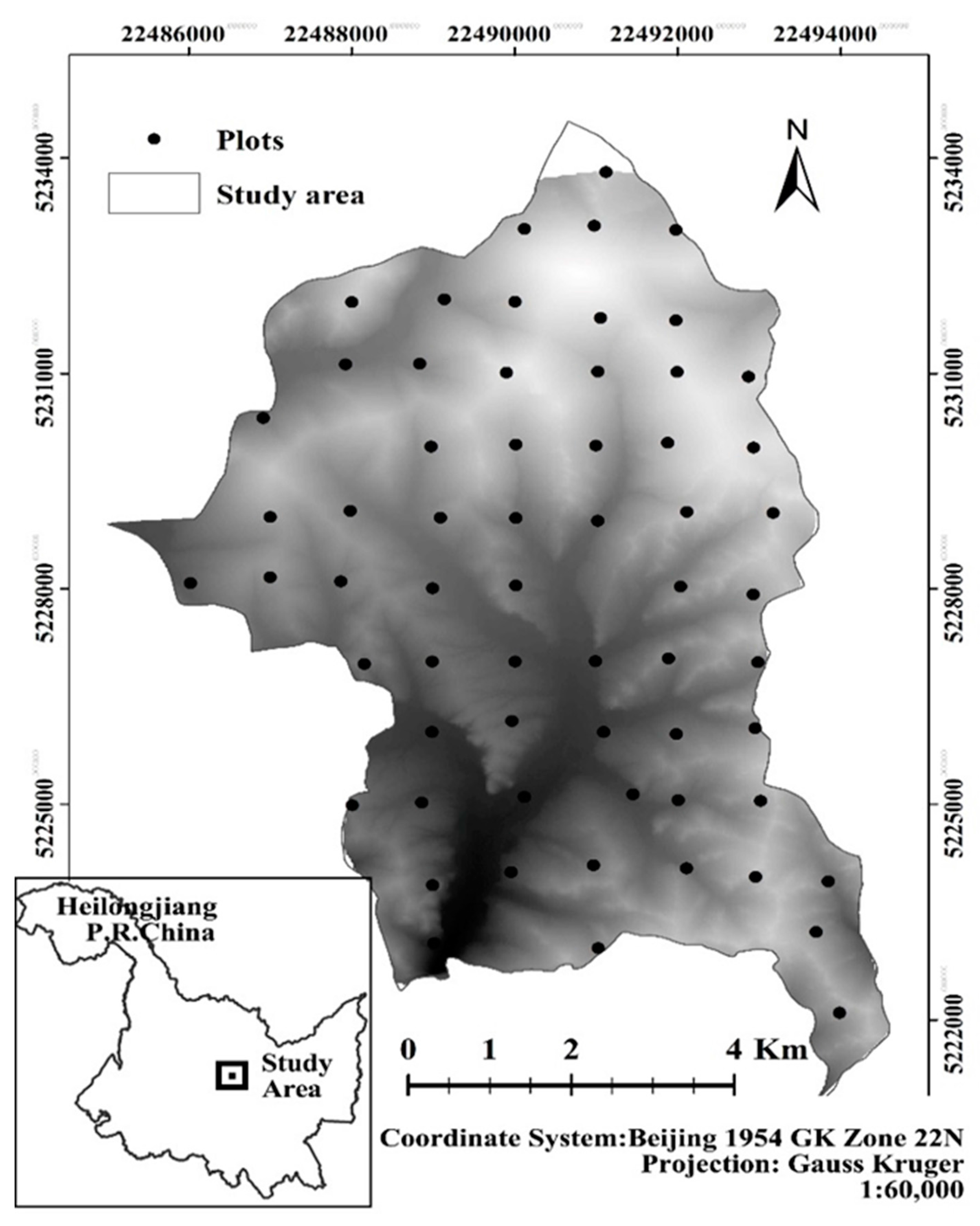
The study site is located at the Liangshui National Nature Reserve, Dailing Distract, Yicun City, Helongjiang Province, P.R. China, extending from 128°47′8″ to 128°57′19″ E in longitude, and from 47°6′49″ to 47°16′10″ N in latitude (Figure 1). The site has a typical temperate continental monsoon climate, with an annual mean temperature of approximately −0.3 °C. The annual mean precipitation is 676 mm, about 60% of which occurs during June and July. The area is characterized by conifer-deciduous mixed forest dominated by Korean pine (Pinus koraiensis), Korean spruce (Picea koraiensis) and fir (Abies nephrolepis) with 50%–60% canopy coverage. Major hardwoods in the area are white birch (Betula platyphylla), Amur corktree (Phellodendrona murense), Northeast China ash (Fraxinus mandshurica), and Manchurian Walnut (Juglans mandshuria). The understory is very clear as a result of forest management every ten years that clears most understory vegetation. The type of soil is Dark-brown soil, which belongs to Argosols Order (Inceptisols) [45]. It develops in conifer–deciduous mixed forests of temperate humid regions. The soil parent materials are mostly weathering materials from granite, andesite, and basalt. The profile type is O-AB-Bt-C, humus is accumulated in the surface, showing a neutrality or sub-acidity reaction; base saturation ranges from 60% to 80%. Clay, ferric and manganese contents in the middle zone are more than those of the upper and lower zones [46].

Figure 1.
Location of the study area and 62 sampling plots.
2.2. Soil Data
The soil data from 62 rectangular plots (0.06 ha each, 20 m × 30 m) were collected in August 2009. The plot centers are located at network intersections of 1 km intervals in the Beijing-54 coordinate system. Furthermore, the plot centers were offset by 50 m when the desired coordinates fell on rivers, roads, landings, or any inaccessible location (Figure 1). In every plot, we used GPS receivers (Garmin 76) to obtain the signals of the real time dynamic differential GPS, and to determine the center coordinate of each plot with a positioning precision of 2 cm. In addition, the distance between GPS receivers and the base station was less than 15 km.
We collected soil samples from the center and four corners in each plot by digging holes (1 m × 1 m) with depths ranging from O (litter layer) to A (organic layer). Subsequently, a steel meter stick was used to determine the depth of the O-A horizon. The soil samples were air dried in separate cloth bags at room temperature (20–30 °C). They were filtered through various sizes of sieves (0.149 and 1 mm) for different analyses. Topsoil properties including SOM, Total N, pH and AvaP were determined, respectively as follows: soil samples filtered through the mesh size of 0.149 mm were used to measure soil organic material by the sulfochromic oxidation approach; soil samples filtered through the mesh size of 0.149 mm were used to measure Total N by elemental analysis method; soil samples filtered through the mesh size of 1 mm were used to determine pH values by the electro-potential method; and soil samples filtered through mesh size of 1 mm were used to determine AvaP using the sodium hydrogen carbonate solution-Mo-Sb anti-spectrophotometric method [45]. Data descriptions of the 62 soil samples are shown in Table 1.

Table 1.
Descriptive statistics of soil samples.
2.3. LiDAR Data
The LiDAR data were acquired in September 2009 using an airborne LiteMapper 5600 laser system. The laser sensor operated at 150 kHz with laser pulse length of 3.5 ns and total scan angle of 14°. Up to four return signals per pulse were recorded by the sensor. More than 50% overlap of adjacent flight lines was applied to obtain a point density of up to 8 points/m2. Raw data were stored in LAS files (format version 1.0). The intensity values of all points (1556 nm laser energy) were rescaled as 8-bit data (0–255). The final points were geo-referenced to the Beijing-54 coordinate system (Table S1).
Pre-processing for classifying ground returns from the raw point clouds was performed by a data vendor (Ingenieur Gesellschaft für Interfaces mbH, Kreuztal, Germany) on the MicroStation Platform using a triangular adaptive-algorithm [47] in TerraScan suites of TerraSoild software (Terrasolid Ltd., Helsinki, Finland). As the forest canopy is not very dense and coverage is 0.5–0.6, most LiDAR pulses can reach the ground. The point density of the extracted ground returns is up to 4 points/m2, and there were enough ground returns to produce the fine scale (1.5 m grid resolution and 3 × 3 neighbor extent) DEM and intensity layer using a kriging interpolate method. For exploring the scale-dependency of soil–topography relationship, the grid resolution and neighbor extent should be taken into consideration. We resampled the DEM and intensity layer to coarser resolutions (10 and 50 m) and larger neighbor extents (5 × 5 and 7 × 7) using a mean resampling method from the raster package in R software, and finally nine scale DEMs and intensity layers were produced for further analysis.
Seven types of topographic factors from the nine scale DEM layers were produced by Whitebox GAT (Version 2.0), and 63 multi-scale topographic variables were generated to further analyze the scale dependency of the soil–topography relationship [48]. The seven types of topographic factors are as follows: elevation, slope, aspect, STI, WI, RSP, and TC (Table S2) [49,50]. Formulas for calculating these topographic variables are as follows:
where Ac is the specific catchment area, namely, the upslope contributing area per unit contour length; β is the local slope gradient in degrees; p is a user-defined exponent term that controls the location-specific relationship between the contributing area and discharge (default, p = 1.0); m is usually set to 0.4; and n is usually set to 1.3.
LiDAR intensity is a function of many factors, such as distance between target and sensor, scanning angle, atmosphere condition, and flight overlapping. Proper processing often depends on the intended application. In this study, we used ENVI LiDAR tools to decrease the influence of flight overlapping on intensity values, calculated the average intensity values of all points to weaken the influence of local terrain, and applied a 3 × 3 median filter [28] to calibrate intensity. However, many studies found that the most important influencing factor for intensity was distance [38,51,52]. We also performed distance normalization of intensity values to calibrate the original intensity to offset the distance-dependency error. This method is widely used and the formula is as follows [51,52]:
where I′ is the normalized intensity, I is the original intensity, R is the distance between sensor and target, and is a standard distance (e.g., 800 m).
2.4. Statistics Analysis
To explore the effectiveness of the aforementioned LiDAR-derived variables for estimating soil properties, Pearson correlation analysis was first performed to indicate the existence of positive or negative relationships between each of the 72 multi-scale predictors and five soil properties, and the variable with the largest value of the correlation coefficients across nine scales was selected as the optimal scale correlated variable for each topsoil property, which showed the scale dependency of the relationships between LiDAR-derived variables and topsoil properties. Then, information theory was used to select the model variables from each scale level (nine resolution-neighbor extent combination scales) and the optimal model across nine scales for each soil property. The information theory approach has been widely accepted for selecting model variables and the optimal models [53,54]. It ranks all possible combinations of variables using the Akaike information criterion (AIC). We therefore selected the subset of variables with the smallest AIC value for the model. Consequently, the model with the smallest AIC value among nine selected models across scales was selected as the optimal model for each soil property [55]. The formulas are as follows:
where k is the number of variables and l is the value of the maximum-likelihood function.
Then, general linear model regression (GLM) was performed for each soil property using the optimal scale model variables selected by the information theory approach. The variance explained by each of the selected predictors was also quantified by an Analysis of Variance (ANOVA) of the GLM. All data were analyzed using the R statistical package (R version 3.1.2). Finally, for exploring the spatial patterns of topsoil properties, we used the “map algebra” module of ArcGIS (version 10.1) to establish the soil maps through calculating the corresponding layers of selected variables with the relationships established by the GLM method for each topsoil property at the optimal scale. The topsoil map for each property was established, which is visual to understand the pattern of each topsoil property.
3. Results
3.1. Correlation Analysis and Variable Selection
Pearson correlation was implemented and the best result of the correlation between 72 multi-scale variables and five topsoil properties was selected and is shown in Table 2. The result suggested that the relationships between intensity and three topsoil properties (SOM, Total N, and pH) were significantly positive ( = 0.80, p < 0.05; = 0.79, p < 0.05; = 0.27, p < 0.05), while intensity was negatively related to Depth ( = −0.51, p < 0.05). Intensity was not, however, significantly related to AvaP.
Table 2.
Best result of Pearson correlation between multi-scale variables and topsoil properties.
There were several types of multi-scale topographic factors that also showed significant relationships with topsoil properties in different scales. Among them, elevation was significantly negatively related to pH and Depth ( = −0.29, p < 0.05; = −0.49, p < 0.05), slope was negatively related to Depth ( = −0.27, p < 0.05), TC was negatively related to SOM and Total N ( = −0.25, p = 0.051; = −0.27, p < 0.05), RSP was negatively related to Total N ( = −0.25, p < 0.05), and STI was significantly negatively related to Depth and AvaP ( = −0.45, p < 0.05; = −0.25, p = 0.053) (Table 2).
Moreover, the results also showed that except for intensity, elevation and RSP, topographic factors had strong scale dependencies for predicting topsoil properties. In general, the topographic factors with coarser grid resolutions and bigger neighbor extents, were more strongly related to five topsoil properties, namely, they had stronger explanatory power for those topsoil properties (Table 2), which supported the conclusions of previous researches [6,7].
Information theory was used to select one optimal scale out of nine scales, one optimal variable or subset of variables, and the optimal model with respect to the selected optimal scale for predicting each topsoil property. The AIC value of each scale model is shown in Table S3. In terms of the principle of minimum AIC values, we selected the optimal subset of variables at an optimal scale for every topsoil property (Table 3). The results showed that the selected variables varied for each topsoil property. SOM and Total N were explained by the same subset of three variables (intensity, elevation and RSP), pH was explained by four variables (intensity, elevation, TC and WI); Depth was explained by intensity, elevation, TC, RSP, STI and WI; and AvaP was weakly explained by three variables (aspect, TC, and STI) (Table 3). The corresponding scales of the selected variables in final models are also shown in Table 3. The results showed that three subsets of selected variables for SOM, Total N, and pH had the same scale, a 1.5 m grid resolution and 4.5 m neighbor extent. Meanwhile, for Depth and AvaP, the two subsets of variables had different scales, which tended to have coarser grid resolutions and larger neighbor extents (Table 3).
Table 3.
The results of selected variables and general linear model regression (GLM).
3.2. GLM Model and Soil Maps
GLM regression was used to further quantify the explanatory power of the selected variables. The results showed that optimal subsets had strong explanatory power for four topsoil properties (SOM, Total N, pH, and Depth), while for AvaP the explanatory power was weak. The percentages of total variations explained for SOM, Total N, pH, Depth and AvaP were 66.3%, 65.8%, 47.1%, 46.4%, and 10.2%, respectively (Table 3).
GLM results also showed that intensity was the strongest predictor of SOM, Total N, and Depth, explaining 17.2% to 63.6% of their variances (Figure 2). In contrast, multi-scale topographic factors explained less of the variance of most topsoil properties; only limited multi-scale topographic variables showed strong explanatory power for relevant topsoil properties. For example, elevation explained 38.3% of the variation of pH with the scale (1.5 m grid resolution and 4.5 m neighbor extent), and STI had strong explanatory power for the variance in Depth (14.5%) with the scale (50 m grid resolution and 250 m neighbor extent). Other single topographic variables had weak explanatory power for relevant topsoil properties with R2 ranging from negligible to 0.072 (Table S4). However, by combining the LiDAR-derived intensity and topographic factors, the prediction accuracies were enhanced by 2.7% to 40.1%. The detailed proportion of variance explained by each predictor is shown in Table S4.
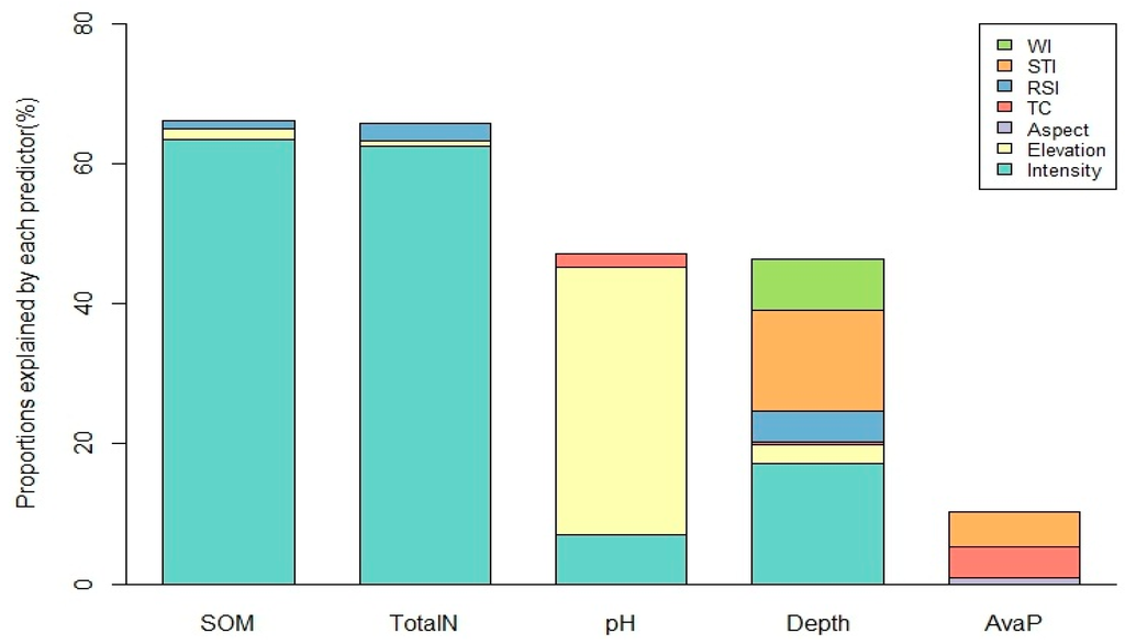
Figure 2.
The proportion of variance explained by each selected variable in the optimal scale. The selected variables for SOM, Total N, and pH have the same scale, which is 1.5 m grid resolution and 4.5 m neighbor extent; the scale of the selected variables for Depth is 50 m grid resolution and 250 m neighbor extent; and the scale of the selected variables for Depth is 10 m grid resolution and 70 m neighbor extent.
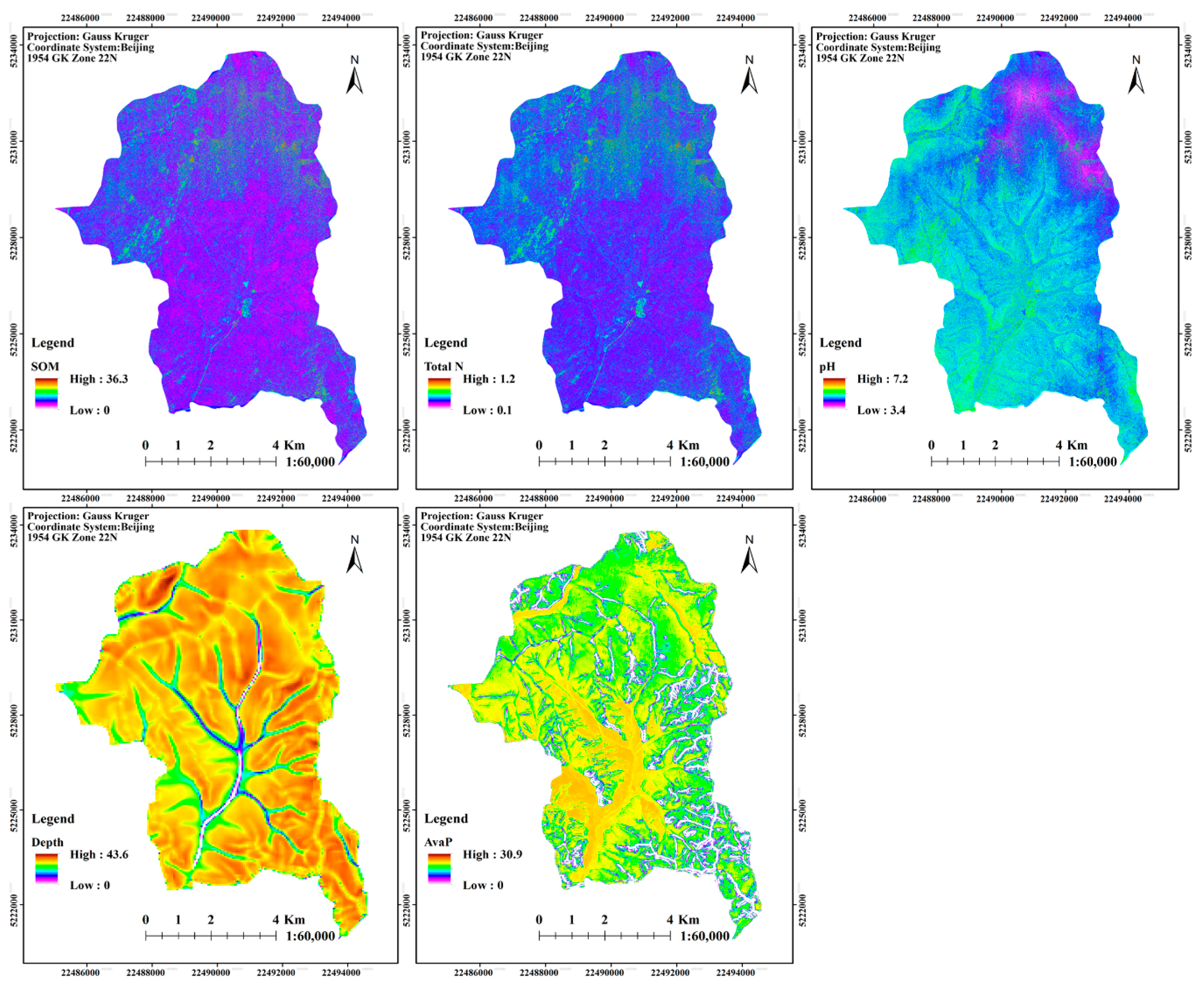
Based on the aforementioned result of GLM, we used the layers of selected variables at optimal scale to establish the soil map for each property, and the result is shown in Figure 3. From the soil maps, the spatial patterns of topsoil properties are visual and easy understandable. Among them, the soil maps of SOM and Total N have the similar spatial patterns, which presents that SOM and Total N have more in north than those in middle and south. pH value is smaller in northeast than in other regions, which means the soil acidity is higher in northeast. In addition, along the ridgelines and streams, the Depth is thinner, while it distributes uniformly in other regions. Moreover, in the middle and low attitude region, the AvaP is higher.

Figure 3.
The soil maps established by each selected variable in the optimal scale. The soil maps for SOM, Total N, and pH have the same scale, which is 1.5 m grid resolution and 4.5 m neighbor extent; the scale of the soil map for Depth is 50 m grid resolution and 250 m neighbor extent; and the scale of the soil map for AvaP is 10 m grid resolution and 70 m neighbor extent.
4. Discussion
4.1. Effects and Scale Dependency of LiDAR Intensity on Topsoil Properties
LiDAR intensity can significantly explain up to 17.2%~63.6% of the variation in three topsoil properties (SOM, Total N, and Depth), but can explain few variances in AvaP and pH (Table S4). This provides robust evidence that LiDAR intensity information is an effective predictor of three topsoil properties and it is even more effective than most topographic factors, which have been widely adopted by previous studies. To the best of our knowledge, this phenomenon has not been reported.
The primary drivers of this phenomenon largely rest on the sensitivity of the spectral reflectance of topsoil properties in the near infrared range (NIR; 800–2100 nm), which covers the working spectral wavelength of our LiDAR system (1550 nm in the NIR range). Former studies using laboratory experiments reported that spectral reflectance of topsoil properties in NIR was sensitive to changes of topsoil property concentrations [15,16,17,18]. In our study, SOM and Total N were strongly correlated with LiDAR intensity values. This makes sense, as LiDAR intensity provides information about the relative proportions of bonds such as C–H and N–H in organic compounds. On the contrary, a recent study reported that the first and last echoes were used to retrieve forest structure metrics, and then those metrics were used to estimate topsoil organic carbon storage. The authors found that topsoil organic carbon was significantly negatively related to intensity [36]. It is worth noting that, in their study area, there was much higher moisture in the soil and the power of LiDAR can probably be absorbed by water in soil. Furthermore, SOM decomposes slowly in such soil because of anaerobic conditions. However, in our study area, those conditions did not exist, topsoil had less moisture, and most of the LiDAR pulses could reach the ground. Under different conditions, we selected proper methods to estimate topsoil properties and obtained different results, which is reasonable.
However, intensity is a poor predictor of AvaP, confirming previous findings [16,17]. This might be associated with the fact that AvaP does not have a primary reflection peak in the NIR region, and the wavelength of 1550 nm is probably insensitive to AvaP levels [56].
Furthermore, when we tried to explore the scale dependency of the intensity–soil relationship, the Pearson correlation analysis showed that intensity had different scale dependencies for predicting each soil property given that the correlation coefficients (r) of different scale intensities ranged from 0.80 to 0.99, and multi-scale intensity layers were significantly and differently related to each other (p < 0.05) (Table S5). With the increasing in the spatial resolution and neighbor extent of intensity layers, their explanatory power for SOM, Total N and Depth declined generally and slightly (Table 1).
Although LiDAR intensity information has functioned well for estimating forest topsoil properties, it also suggested that intensity data should be calibrated using proper methods prior to applications, especially for quantitative analysis. Moreover, scale dependencies of relationships between intensity and soil properties were weak in our study, except for Depth. Intensity in finest scale, however, had better explanatory power for Depth than that for the scale, providing a 50 m grid resolution and 250 m neighbor extent. On the contrary, the selected subset of topographic factors had the opposite result for Depth. This phenomenon, however, deserves attention in future studies with respect to scale-related properties (Table S6).
4.2. Effects and Scale Dependency of Topographic Factors on Topsoil Properties
The relationships varied, which were between seven types of selected multi-scale topographic factors and five topsoil properties. The R2 values of optimal models ranged from negligible to 0.38 (Table S4), a similar correlation to those reported by previous studies [4,8,10]. Among topographic factors, elevation had a significantly negative correlation with pH ( = −0.49, p < 0.05), confirming the conclusions of previous works [11,14,57]. Notice that elevation explained 24% of the variance of pH in previous research [57], and similarly, it explained up to 38% in our study. Besides, STI had a significantly negative correlation with Depth, and it could explain 14.5% of the variance in Depth. This phenomenon is understandable, given that STI represents the capability of soil erosion, namely, a larger STI value means stronger soil erosion [4,58], which obviously leads to a decrease in soil Depth.
Furthermore, to compare the explanatory powers of the multi-scale selected subsets of topographic factors for topsoil properties, we used the selected subsets of topographic factors with the finest scale (1.5 m grid resolution and 4.5 m neighbor extent) as the baseline. This result showed that using optimal scale subsets of topographic factors to predict topsoil properties, the prediction accuracies were enhanced by negligible amounts up to 20.2% (Table S7). However, elevation, RSP and WI had no significant scale dependency on predicting topsoil properties, as the correlation coefficients among multi-scale elevations were 0.998 at least (Table S8), while RSP and WI varied greatly across spatial scales (Tables S9 and S10). In conclusion, elevation is insensitive to scale, while RSP and WI are sensitive to scales, although they have weak explanatory power for the five topsoil properties (Table S6). Moreover, it is possible that our study missed the best spatial scale of RSP and WI for predicating topsoil properties, given that only three spatial scales were considered in this study. This phenomenon is worth noting in further studies.
In summary, the explanatory powers of multi-scale topographic factors varied for predicting topsoil properties, and they should be selected carefully in future applications. Moreover, topographic factors except elevation, RSP, and WT had strong scale dependency with respect to topsoil properties, and we should take scale dependency of soil–topography into consideration when we use LiDAR data to quantitatively retrieve topsoil properties or other similar features (topsoil structure, texture, moisture, etc.) in the future. Furthermore, elevation and RSP might have different scale effects for soil properties, and they should be treated differently. In addition, the topsoil maps showed that the spatial patterns were different for properties across scales, and soil maps were important products to visually exhibit the relationship between selected variables and the corresponding topsoil property. The soil maps, therefore, should be established, when we study the relationships between various retrieval variables and soil properties.
5. Conclusions
To explore the effectiveness of LiDAR-derived variables for predicting topsoil properties, we used information theory method to select the optimal scale, variables, and models, and established GLM for topsoil properties. This would be a great approach to select an optimal spatial scale of topographic factors for model development. Overall, we obtained several conclusions: (1) LiDAR intensity was an effective predictor of three topsoil properties (SOM, Total N, and Depth) with R2 ranging from 0.17 to 0.64; (2) multi-scale LiDAR-derived topographic factors had different explanatory powers for the five topsoil properties with R2 ranging from negligible to 0.38, and elevation was a robust predictor for pH with R2 of 0.38; (3) when combinations of intensity and LiDAR-derived topographic factors were applied, the prediction accuracies (R2) could be enhanced by negligible amounts up to 0.40, relative to only using intensity for topsoil properties; and (4) the prediction accuracy for Depth increased by 0.20, while for other topsoil properties the prediction accuracies increased negligibly when the scale dependency of the soil–topography relationship was considered.
The aforementioned findings suggest that LiDAR intensity is a valuable predictor for topsoil properties in forests with complicated topography and dense canopy cover. This study might therefore enhance our understanding of the utility of LiDAR intensity in forest soil related areas and extend its application in forest ecology.
Supplementary Materials
The following are available online at www.mdpi.com/2072-4292/8/7/561/s1, Table S1: LiDAR system parameters, Table S2: Description of eight LiDAR-derived variables, Table S3: Nine scale candidate models with Akaike information criterion (AIC), Table S4: Proportion of variance explained by each selected predictor in Table S3, Table S5: Pearson correlation analysis result of nine scale intensities, Table S6: Proportion of each topsoil property explained by each variable in optimal scale models and baseline scale models, Table S7: Comparison of the optimal scale model and the baseline scale model for each topsoil property, Table S8: Pearson correlation analysis result of nine scale Elevations, Table S9: Pearson correlation analysis result of nine scale RSPs, Table S10: Pearson correlation analysis result of nine scale WIs.
Acknowledgments
The paper was sponsored by the Fundamental Research Funds for the Central Universities (Grant No. 2572016CA01) and the National “Twelfth Five-Year” Plan for Science & Technology Support Program (Grant No. 2012BAD22B0202) granted to Zhaogang Liu, and the National Natural Science Foundation of China (Grant No. 31321061) granted to Jingyun Fang. We are also grateful to all colleagues and students of Northeast Forestry University, who took part in the field measured forest surveying in August 2009.
Author Contributions
Chao Li and Zhaogang Liu conceived and designed the experiments; Chao Li and Yanli Xu performed the experiments and analyzed the data; and Chao Li, Zhaogang Liu, Shengli Tao, Fengri Li, and Jingyun Fang wrote the paper.
Conflicts of Interest
The authors declare no conflict of interest.
Abbreviations
The following abbreviations are used in this manuscript:
| LiDAR | Light Detection and Ranging |
| SOM | Soil Organic Matter |
| Total N | Total Nitrogen |
| pH | pH value |
| Depth | O-A horizon Depth |
| AvaP | available phosphorous |
| 3D | three-dimensional |
| DEM | digital elevation model |
| R2 | Coefficient of determination |
| NIR-SWIR | Near Infrared to Short Wave Infrared |
| WI | Topographic Wetness Index |
| RSP | Relative Stream Power Index |
| STI | Sediment Transport Index |
| TC | Total Curvature |
| GPS | Global Positioning System |
| AIC | Akaike Information Criterion |
| GLM | General Linear Model regression |
References
- Susanne, A.; Wander, M.M. Long-Term Trends of Corn Yield and Soil Organic Matter in Different Crop Sequences and Soil Fertility Treatments on the Morrow Plots. Adv. Agron. 1997, 62, 153–197. [Google Scholar]
- Zhang, S.; Huang, Y.; Shen, C.; Ye, H.; Du, Y. Spatial prediction of soil organic matter using terrain indices and categorical variables as auxiliary information. Geoderma 2012, 171–172, 35–43. [Google Scholar] [CrossRef]
- McBratney, A.B.; Santos, M.M.; Minasny, B. On digital soil mapping. Geoderma 2003, 117, 3–52. [Google Scholar] [CrossRef]
- Moore, I.D.; Gessler, P.E.; Nielsen, G.A.; Peterson, G.A. Soil attribute prediction using terrain analysis. Soil Sci. Soc. Am. J. 1993, 57, 443–452. [Google Scholar] [CrossRef]
- Kienzle, S. The effect of DEM raster resolution on first order, second order and compound terrain derivatives. Trans. GIS 2004, 8, 83–111. [Google Scholar] [CrossRef]
- Maynard, J.J.; Johnson, M.G. Scale-dependency of LiDAR derived terrain attributes in quantitative soil-landscape modeling: Effects of grid resolution vs. neighborhood extent. Geoderma 2014, 230, 29–40. [Google Scholar] [CrossRef]
- Miller, B.A.; Koszinski, S.; Wehrhan, M.; Sommer, M. Impact of multi-scale predictor selection for modeling soil properties. Geoderma 2015, 239, 97–106. [Google Scholar] [CrossRef]
- Lin, Y.; Prentice, S.E.; Tran, T.; Bingham, N.L.; King, J.Y.; Chadwick, O.A. Modeling deep soil properties on California grassland hillslopes using LiDAR digital elevation models. Geoderma Reg. 2016, 7, 67–75. [Google Scholar] [CrossRef]
- Herbst, M.; Diekkrüger, B.; Vereecken, H. Geostatistical co-regionalization of soil hydraulic properties in a micro-scale catchment using terrain attributes. Geoderma 2006, 132, 206–221. [Google Scholar] [CrossRef]
- Takata, Y.; Funakawa, S.; Akshalov, K.; Ishida, N.; Kosaki, T. Spatial prediction of soil organic matter in northern Kazakhstan based on topographic and vegetation information. Soil Sci. Plant Nutr. 2007, 53, 289–299. [Google Scholar] [CrossRef]
- Griffiths, R.P.; Madritch, M.D.; Swanson, A.K. The effects of topography on forest soil characteristics in the Oregon Cascade Mountains (USA): Implications for the effects of climate change on soil properties. Forest Ecol. Manag. 2009, 257, 1–7. [Google Scholar] [CrossRef]
- Kumhálová, J.; Kumhála, F.; Kroulík, M.; Matějková, Š. The impact of topography on soil properties and yield and the effects of weather conditions. Precis. Agric. 2011, 12, 813–830. [Google Scholar] [CrossRef]
- Wang, S.; Wang, X.; Ouyang, Z. Effects of land use, climate, topography and soil properties on regional soil organic carbon and total nitrogen in the Upstream Watershed of Miyun Reservoir, North China. J. Environ. Sci. 2012, 24, 387–395. [Google Scholar] [CrossRef]
- Qi-yong, Y.; Zhong-cheng, J.; Wen-jun, L.; Hui, L. Prediction of soil organic matter in peak-cluster depression region using kriging and terrain indices. Soil Tillage Res. 2014, 144, 126–132. [Google Scholar] [CrossRef]
- Palacios-Orueta, A.; Ustin, S.L. Remote sensing of soil properties in the Santa Monica Mountains I. Spectral analysis. Remote Sens. Environ. 1998, 65, 170–183. [Google Scholar] [CrossRef]
- Chang, C.-W.; Laird, D.A.; Mausbach, M.J.; Hurburgh, C.R. Near-infrared reflectance spectroscopy–principal components regression analyses of soil properties. Soil Sci. Soc. Am. J. 2001, 65, 480–490. [Google Scholar] [CrossRef]
- Islam, K.; Singh, B.; McBratney, A. Simultaneous estimation of several soil properties by ultra-violet, visible, and near-infrared reflectance spectroscopy. Soil Res. 2003, 41, 1101–1114. [Google Scholar] [CrossRef]
- McCarty, G.W.; Reeves, J.B. Comparison of near infrared and mid infrared diffuse reflectance spectroscopy for field-scale measurement of soil fertility parameters. Soil Res. 2006, 171, 94–102. [Google Scholar] [CrossRef]
- Lefsky, M.A.; Cohen, W.B.; Harding, D.J.; Parker, G.G.; Acker, S.A.; Gower, S.T. Lidar remote sensing of above-ground biomass in three biomes. Glob. Ecol. Biogeogr. 2002, 11, 393. [Google Scholar] [CrossRef]
- Patenaude, G.; Hill, R.A.; Milne, R.; Gaveau, D.L.A.; Briggs, B.B.J.; Dawson, T.P. Quantifying forest above ground carbon content using LiDAR remote sensing. Remote Sens. Environ. 2004, 93, 368–380. [Google Scholar] [CrossRef]
- Müller, J.; Brandl, R. Assessing biodiversity by remote sensing in mountainous terrain: The potential for LiDAR to predict forest beetle assemblages. J. Appl. Ecol. 2009, 46, 897–905. [Google Scholar] [CrossRef]
- Bässler, C.; Stadler, J.; Müller, J.; Förster, B.; Göttlein, A.; Brandl, R. LiDAR as a rapid tool to predict forest habitat types in Natura 2000 networks. Biodivers. Conserv. 2011, 20, 465–481. [Google Scholar] [CrossRef]
- Wolf, G. LiDAR Goes Mainstream. In Transmission & Distribution World; Penton Business Media, Inc.: Overland Park, KS, USA, 2011. [Google Scholar]
- Hodgson, M.E.; Jensen, J.R.; Schmidt, L.; Schill, S.; Davis, B. An evaluation of LIDAR- and IFSAR-derived digital elevation models in leaf-on conditions with USGS Level 1 and Level 2 DEMs. Remote Sens. Environ. 2003, 84, 295–308. [Google Scholar] [CrossRef]
- Töyrä, J.; Pietroniro, A. Towards operational monitoring of a northern wetland using geomatics-based techniques. Remote Sens. Environ. 2005, 97, 174–191. [Google Scholar] [CrossRef]
- Murphy, P.N.C.; Ogilvie, J.; Meng, F.-R.; White, B.; Bhatti, J.S.; Arp, P.A. Modelling and mapping topographic variations in forest soils at high resolution: A case study. Ecol. Model. 2011, 222, 2314–2332. [Google Scholar] [CrossRef]
- Smeeckaert, J.; Mallet, C.; David, N.; Chehata, N.; Ferraz, A. Large-scale classification of water areas using airborne topographic lidar data. Remote Sens. Environ. 2013, 138, 134–148. [Google Scholar] [CrossRef]
- Song, J.; Han, S.; Yu, K.; Kim, Y. Assessing the possibility of land-cover classification using LiDAR intensity data. In Proceedings of the ISPRS Commission III, Graz, Austria, 9–13 September 2002.
- Yoon, J.S.; Shin, J.I.; Lee, K.S. Land cover characteristics of airborne LiDAR intensity data: A case study. IEEE Geosci. Remote Sens. Lett. 2008, 5, 801–805. [Google Scholar] [CrossRef]
- Yan, W.Y.; Shaker, A.; Habib, A.; Kersting, A.P. Improving classification accuracy of airborne LiDAR intensity data by geometric calibration and radiometric correction. ISPRS J. Photogramm. Remote Sens. 2012, 67, 35–44. [Google Scholar] [CrossRef]
- Andersen, H.-E.; Reutebuch, S.E.; McGaughey, R.J.; d’Oliveira, M.V.N.; Keller, M. Monitoring selective logging in western Amazonia with repeat lidar flights. Remote Sens. Environ. 2014, 151, 157–165. [Google Scholar] [CrossRef]
- Coren, F.; Sterzai, P. Radiometric correction in laser scanning. Int. J. Remote Sens. 2006, 27, 3097–3104. [Google Scholar] [CrossRef]
- Streutker, D.R.; Glenn, N.F. LiDAR measurement of sagebrush steppe vegetation heights. Remote Sens. Environ. 2006, 102, 135–145. [Google Scholar] [CrossRef]
- Sun, G.; Ranson, K.; Guo, Z.; Zhang, Z.; Montesano, P.; Kimes, D. Forest biomass mapping from lidar and radar synergies. Remote Sens. Environ. 2011, 115, 2906–2916. [Google Scholar] [CrossRef]
- Lang, M.W.; McCarty, G.W. Lidar intensity for improved detection of inundation below the forest canopy. Wetlands 2009, 29, 1166–1178. [Google Scholar] [CrossRef]
- Grebby, S.; Cunningham, D.; Naden, J.; Tansey, K. Lithological mapping of the Troodos ophiolite, Cyprus, using airborne LiDAR topographic data. Remote Sens. Environ. 2010, 114, 713–724. [Google Scholar] [CrossRef]
- Moffiet, T.; Mengersen, K.; Witte, C.; King, R.; Denham, R. Airborne laser scanning: Exploratory data analysis indicates potential variables for classification of individual trees or forest stands according to species. ISPRS J. Photogramm. Remote Sens. 2005, 59, 289–309. [Google Scholar] [CrossRef]
- Donoghue, D.N.M.; Watt, P.J.; Cox, N.J.; Wilson, J. Remote sensing of species mixtures in conifer plantations using LiDAR height and intensity data. Remote Sens. Environ. 2007, 110, 509–522. [Google Scholar] [CrossRef]
- Antonarakis, A.S.; Richards, K.S.; Brasington, J. Object-based land cover classification using airborne LiDAR. Remote Sens. Environ. 2008, 112, 2988–2998. [Google Scholar] [CrossRef]
- Kristensen, T.; Næsset, E.; Ohlson, M.; Bolstad, P.V.; Kolka, R. Mapping Above- and Below-Ground Carbon Pools in Boreal Forests: The Case for Airborne Lidar. PLoS ONE 2015, 10, e0138450. [Google Scholar] [CrossRef] [PubMed]
- Kaasalainen, S.; Pyysalo, U.; Krooks, A.; Vain, A.; Kukko, A.; Hyyppä, J.; Kaasalainen, M. Absolute Radiometric Calibration of ALS Intensity Data: Effects on Accuracy and Target Classification. Sensors 2011, 11, 10586–10602. [Google Scholar] [CrossRef] [PubMed]
- Southee, F.; Treitz, P.M.; Scott, N.A. Application of Lidar terrain surfaces for soil moisture modeling. Photogramm. Eng. Remote Sens. 2012, 78, 1241–1251. [Google Scholar] [CrossRef]
- Turner, R.; Panciera, R.; Tanase, M.A.; Lowell, K.; Hacker, J.M.; Walker, J.P. Estimation of soil surface roughness of agricultural soils using airborne LiDAR. Remote Sens. Environ. 2014, 140, 107–117. [Google Scholar] [CrossRef]
- Challis, K.; Carey, C.; Kincey, M.; Howard, A.J. Airborne lidar intensity and geoarchaeological prospection in river valley floors. Archaeol. Prospect. 2011, 18, 1–13. [Google Scholar] [CrossRef]
- Brady, N.C.; Weil, R.R. Elements of the Nature and Properties of Soils; Pearson Educational Incorporated: Upper Saddle River, NJ, USA, 2004. [Google Scholar]
- Liu, H.W.; Ding, Y.H. Analysis of daily precipitation characteristics over North China during rainy seasons. Chin. J. Atmosp. Sci. 2010, 34, 12–22, (In Chinese with English abstract). [Google Scholar]
- Soininen, A. TerrasScan User’s Guide; Terrasolid: Helsinki, Finland, 2005. [Google Scholar]
- Lindsay, J.B. The Whitebox Geospatial Analysis Tools project and open-access GIS. In Proceedings of the GIS Research 22nd UK Annual Conference, Glasgow, UK, 16–18 April 2014.
- Rinaldo, A.; Rodriguez-Iturbe, I.; Rigon, R.; Bras, R.L.; Ijjasz-Vasquez, E.; Marani, A. Minimum energy and fractal structures of drainage networks. Water Resour. Res. 1992, 28, 2183–2195. [Google Scholar] [CrossRef]
- Moore, I.D.; Burch, G.J. Physical basis of the length-slope factor in the Universal Soil Loss Equation. Soil Sci. Soc. Am. J. 1986, 50, 1294–1298. [Google Scholar] [CrossRef]
- Starek, M.; Luzum, B.; Kumar, R.; Slatton, K.C. Normalizing Lidar Intensities. GEM Center Report No. Rep_2006-12-001; University of Florida: Gainesville, FL, USA, 2006. [Google Scholar]
- García, M.; Riaño, D.; Chuvieco, E.; Danson, F.M. Estimating biomass carbon stocks for a Mediterranean forest in central Spain using LiDAR height and intensity data. Remote Sens. Environ. 2010, 114, 816–830. [Google Scholar] [CrossRef]
- Wang, Z.; Fang, J.; Tang, Z.; Lin, X. Patterns, determinants and models of woody plant diversity in China. Proc. Biol. Sci. 2011, 278, 2122–2132. [Google Scholar] [CrossRef] [PubMed]
- Tao, S.; Fang, J.; Zhao, X.; Zhao, S.; Shen, H.; Hu, H.; Tang, Z.; Wang, Z.; Guo, Q. Rapid loss of lakes on the Mongolian Plateau. Proc. Natl. Acad. Sci. USA 2015, 112, 2281–2286. [Google Scholar] [CrossRef] [PubMed]
- Burnham, K.P.; Anderson, D.R. Model-Selection and Multi-Model Inference: A Practical Information-Theoretic Approach; Springer: New York, NY, USA, 2002. [Google Scholar]
- Confalonieri, M.; Fornasier, F.; Ursino, A.; Boccardi, F.; Pintus, B.; Odoardi, M. The potential of near infrared reflectance spectroscopy as a tool for the chemical characterisation of agricultural soils. J. Near Infrared Spectrosc. 2001, 9, 123–131. [Google Scholar] [CrossRef]
- Jenny, H. The Soil Resource, Origin and Behavior; Springer-Verlag: New York, NY, USA, 1980. [Google Scholar]
- Yoo, K.; Amundson, R.; Heimsath, A.M.; Dietrich, W.E. Spatial patterns of soil organic carbon on hillslopes: Integrating geomorphic processes and the biological C cycle. Geoderma 2006, 130, 47–65. [Google Scholar] [CrossRef]

© 2016 by the authors; licensee MDPI, Basel, Switzerland. This article is an open access article distributed under the terms and conditions of the Creative Commons Attribution (CC-BY) license (http://creativecommons.org/licenses/by/4.0/).