Discrimination between Ground Vegetation and Small Pioneer Trees in the Boreal-Alpine Ecotone Using Intensity Metrics Derived from Airborne Laser Scanner Data

Abstract

It has been shown that height measurements obtained by airborne laser scanning (ALS) with high point density (>7–8 m⁻²) can be used to detect small trees in the alpine tree line—an ecotone sensitive to climate change. Because the height measurements do not discriminate between trees and other convex structures with positive height values, this study aimed at assessing the contribution of ALS backscatter intensity to classification of trees and non-trees. The study took place in a boreal-alpine ecotone in southeastern Norway and was based on 500 precisely georeferenced small trees and non-tree objects for which ALS height and intensity were derived from four different ALS acquisitions, representing different sensors, pulse repetition frequencies (PRF), and flying altitudes. The sensors operated at 1064 nm. Based on logistic regression modeling, it was found that classification into three different tree species ((1) spruce; (2) pine; and (3) birch)) and two different non-tree object types (objects with: (1) vegetated surface; and (2) rock) was significantly better (p < 0.001–0.05) than a classification based on models with trees and non-trees as binary response. The cause of the improved classification is mainly diverse reflectivity properties of non-tree objects. No effect of sensor, PRF, and flying altitude was found (p > 0.05). Finally, it was revealed that in a direct comparison of the contribution of intensity backscatter to improve classification models of trees and non-trees beyond what could be obtained by using the ALS height information only, the contribution of intensity turned out to be far from significant (p > 0.05). In conclusion, ALS backscatter intensity seems to be of little help in classification of small trees and non-trees in the boreal-alpine ecotone even when a more detailed discrimination on different species and different non-tree structures is applied.

1. Introduction

Airborne laser scanning (ALS) is a rapidly growing technology in operational forest inventory at various geographical scales [1,2,3,4]. It also holds potentials for forest monitoring [5,6], ecological applications and biodiversity assessment [7,8], and for monitoring of effects of global warming in those biomes for which changes are expected to be significant over a fairly short time period, like in the transition zones between the boreal forest and the alpine region [9]. In these transition zones, even a moderate change in temperature may lead to a rapid increase in growth of existing trees as well as colonization of tree-less areas due to the steep temperature-productivity gradients that exist in these zones [10,11,12].

Monitoring of changes in vegetation communities and extent of forests is challenging with any remote sensing technique, especially at detailed and local scales. Recently, it has been advocated and even demonstrated empirically that airborne laser scanning is capable of discerning individual small trees forming the tree lines in the boreal-alpine [9] and tundra-taiga interfaces [13] and assist in estimation of tree biomass in the forest-tundra ecotone [14]. Using ALS data with a point density of 7.7 points per m², Næsset and Nelson [9] found that >90% of the trees could be identified when they had reached a height of 1 m or higher. Based on a preliminary investigation using data from a scanning laser with low density (~0.25 points per m²), Rees [13] anticipated that ALS could provide a means for discerning individual trees—defined by a height of >2 m, over hundreds of square kilometers. In the study by Næsset and Nelson [9], the height of the laser echoes was used as criterion for discerning the trees. A height value of a laser echo greater than zero above the modeled terrain surface was assumed to represent a tree hit. No attempt was made to classify the objects that were identified according to a criterion based on height. For laser echo heights >1 m, however, there are usually very few other objects but trees that reach such an elevation above the terrain. Thus, for trees taller than, say, 1 m, the height value is a fairly reliable criterion for tree detection in most environments in the alpine tree line. For smaller trees (<1 m), Næsset and Nelson [9] reported that 5%–73% of the trees appeared to have laser echoes with heights >0 m, depending on tree species and the degree of smoothing when deriving the terrain model that serves as reference surface for the laser height measurements. For such small trees, the uncertainty of the terrain surface itself also becomes an issue as trees smaller than, say, 0.1–0.3 m in height in most cases will be within the confidence bounds of the modeled terrain surface [15,16]. It is nevertheless important to be able to detect such trees as far as possible as they may be early warning signals of temperature-induced changes in the tree line. Immediate responses to short-term changes in temperature, length of growing season, precipitation patterns, and nitrogen deposition from air pollution seem to be present also for larger forest-forming trees for which ALS can be a useful technique to quantify changes [17].

To improve detection and identification of individual small trees, additional criteria for classification might be considered. A natural choice would be to consider spectral information. Identification of tree species or species groups is fundamental in forest resource assessment and in forest ecosystem classification. In remote sensing, discrimination between different tree species is a great challenge with most sensor technologies.

Quite often spectral data from digital imagery with high geometrical resolution is available—either as data from a separate acquisition or as part of the ALS campaign whenever the ALS sensor has an integrated camera system in use. However, spectral information is usually available as part of the ALS dataset itself when a state-of-the-art ALS sensor is applied. Most ALS sensors record the intensity of the backscatter signal [18]. For pulse lasers, intensity often represents the peak amplitude of the returned pulse. Although it was demonstrated already in the mid 1980s that intensity from airborne lasers could assist in classification of individual trees into conifers and broadleaves [19], further development has been hampered by lack of methods for radiometric calibration of the intensity [20]. Lately, there is evidence of various intensity variables from ALS providing useful information for tree species classification [21,22,23,24,25,26,27].

Although discrimination between tree species may assist in separating trees from terrain structures and non-terrain objects, addressing the differences between trees and non-trees directly might be a useful strategy. Thus, it was shown by Korpela [28] that understory lichens could be separated from other ground vegetation using raw intensity values from ALS as well as normalized intensity. The normalized data performed best, though, with a classification accuracy of up to ~75% against an accuracy of ~70% for raw values. These results may indicate that intensity data from ALS potentially could be used for discriminating between small trees and certain types of ground vegetation as well since lichens is a quite frequently occurring ground vegetation in the alpine tree line. ALS backscatter intensity has also been considered as one among several spectral variables for classification of seedling stand vegetation [15] and boreal mire vegetation [29].

In Korpela’s study [28], it was shown that light lichens like the common Cladina (reindeer) lichen had a higher reflectivity than the contrasting ground vegetation using an ALS system with a wavelength of 1064 nm. The contrasting vegetation consisted of mosses and a shrub layer of heather (Calluna vulgaris), lingonberry (Vaccinium vitis-idaea), and crowberry (Empetrum nigrum). These are also among the most common species in the boreal-alpine ecotone in Scandinavia. The fact that these species might have a slightly lower reflectivity at 1064 nm than light lichens and probably a reflectivity not very different from small trees (<1 m), especially deciduous trees like birch, may indicate that discriminating between small trees and non-trees might be more difficult for certain types of ground vegetation.

The potential of backscatter intensity to improve tree and vegetation classification led Stumberg et al. [30] to include backscatter intensity in addition to ALS echo height in classification models for small trees and non-tree objects. Intensity was shown to be a statistically significant variable in the models, but although they also tested classification models ignoring intensity as a potential variable [31], a significant contribution of intensity to improve the classification beyond a classification using only height-related information was not documented. Because establishment of new small trees in the boreal-alpine ecotone hardly is a random process but is governed partly by environmental factors related to for example wind speed, wind direction, and snow-cover, additional variables such as slope and aspect and spatial properties of echo height and backscatter intensity were evaluated in the modeling [30,32]. Intensity in its simple form, i.e., ignoring the spatial patterns of the intensity, remained the second strongest predictor for classification purposes next to echo height.

Monitoring of vegetation has often a long-term perspective. Due to rapid technological development, ALS sensors have a limited commercial lifetime or are subject to frequent upgrades. Thus, in a monitoring context different instruments will typically be used at different points in time. When using different ALS instruments and different acquisition parameters like flying altitude and pulse repetition frequency, the acquired intensity values will tend to change because of different properties of the emitted pulse, such as pulse energy, pulse width, and peak power. Korpela [28] found different reflectivities of the vegetation backscatter using two different instruments, i.e., an Optech ALTM 3100 and a Leica ALS 50-II sensor. Because the pulse properties will change significantly for a given sensor with changing acquisition parameters [33], the ranging will be influenced [34] and so will also the intensity of the backscatter since the energy of the emitted pulse will change. It is therefore likely that different sensors and acquisitions accomplished with different settings may perform differently when using backscatter intensity to discriminate between small trees and non-trees.

In the studies by Stumberg et al. [30,32], it was not distinguished between different tree species and it was not distinguished between different non-tree objects in the modeling and classification. Because the spectral properties vary between tree species as well as between different non-tree objects, the first objective of the current study (Objective A) was to evaluate if classification into individual tree species and individual types of non-tree objects could improve the overall performance of a binary tree/non-tree classification. Such potential improvements might suggest that use of for example multispectral imagery or even hyperspectral data in combination with ALS could be beneficial, cf. [35].

The second objective (Objective B) was to assess to what extent classification performance of trees and non-trees was influenced by different sensor and flight configurations.

Finally, the third objective (Objective C) was test the performance of classification of trees vs. non-trees utilizing both height and intensity to mimic a real inventory situation, allowing a quantification of the contribution of intensity data to the overall classification performance. Recently, a practical procedure to segmented trees (small objects) was proposed [36], but it remains unknown to what extent backscatter intensity could improve the classification of segmented objects into trees and non-trees.

2. Materials and Methods

This study was based on previously published field data collected in 2006 [9] supplemented by new and currently unpublished data collected in 2010. The ALS data used in the current research were acquired in 2006 [9] and 2007 [34]. However, while the previous studies only focused on the ALS ranging measurements, the current work deals with intensity of the backscatter signal. For thorough descriptions of the field data and the ALS sensor and flight configurations, the reader is referred to [9,34], respectively. An overview is given below though, along with a primary documentation of the field data collected in 2010.

2.1. Study Area

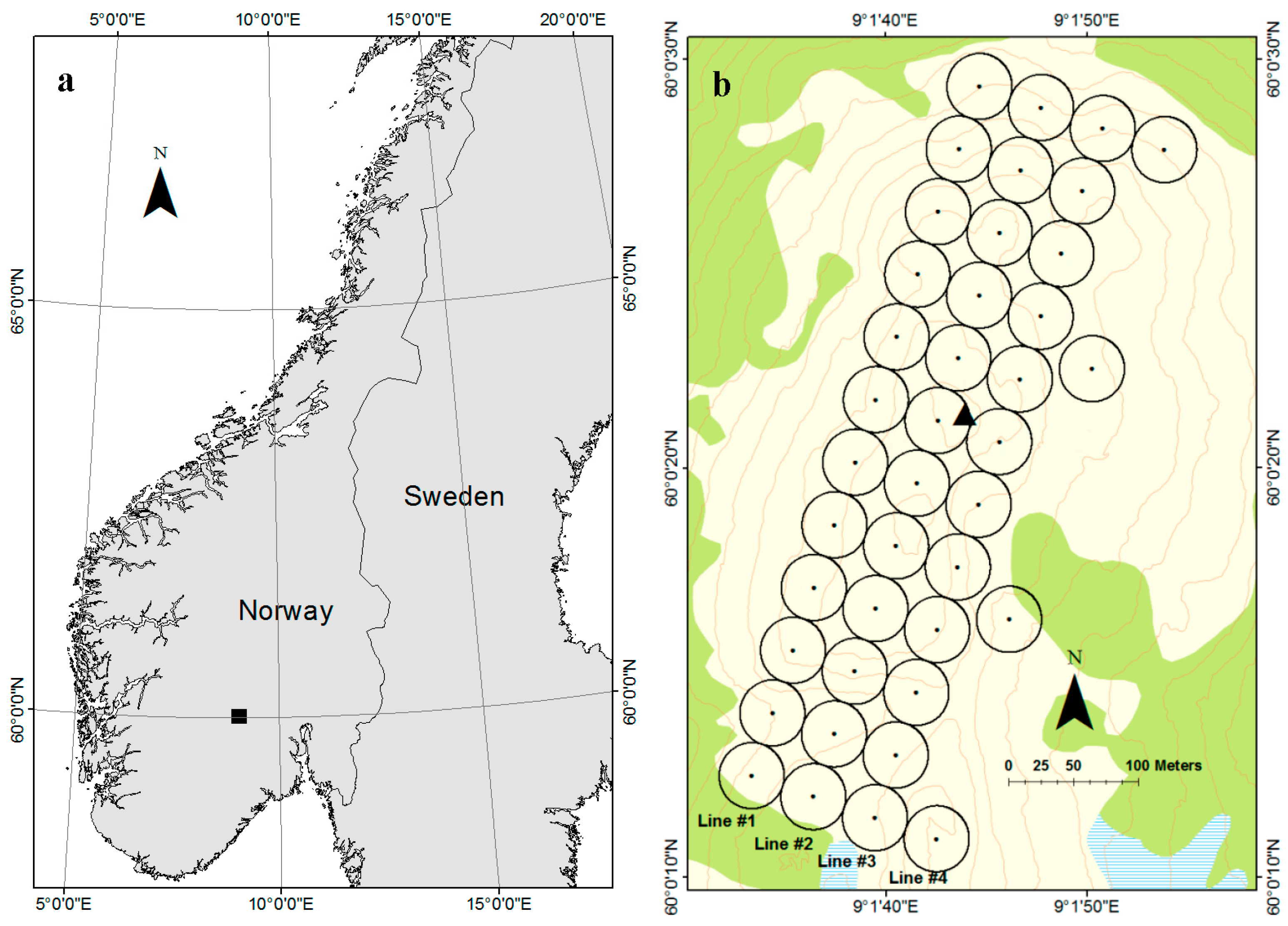
The study area is located on a small mountain ridge in the municipality of Rollag, southeastern Norway (60°0′N 9°01′E, 910–950 m above sea level). The entire study was conducted within a rectangle of size 200 m × 600 m. The work took place in the tree line, which at this location is around 900–940 m above sea level. The main tree species in the trial area are Norway spruce (Picea abies (L.) Karst.), Scots pine (Pinus sylvestris L.), and mountain birch (Betula pubescens ssp. czerepanovii).

2.2. Field Measurements

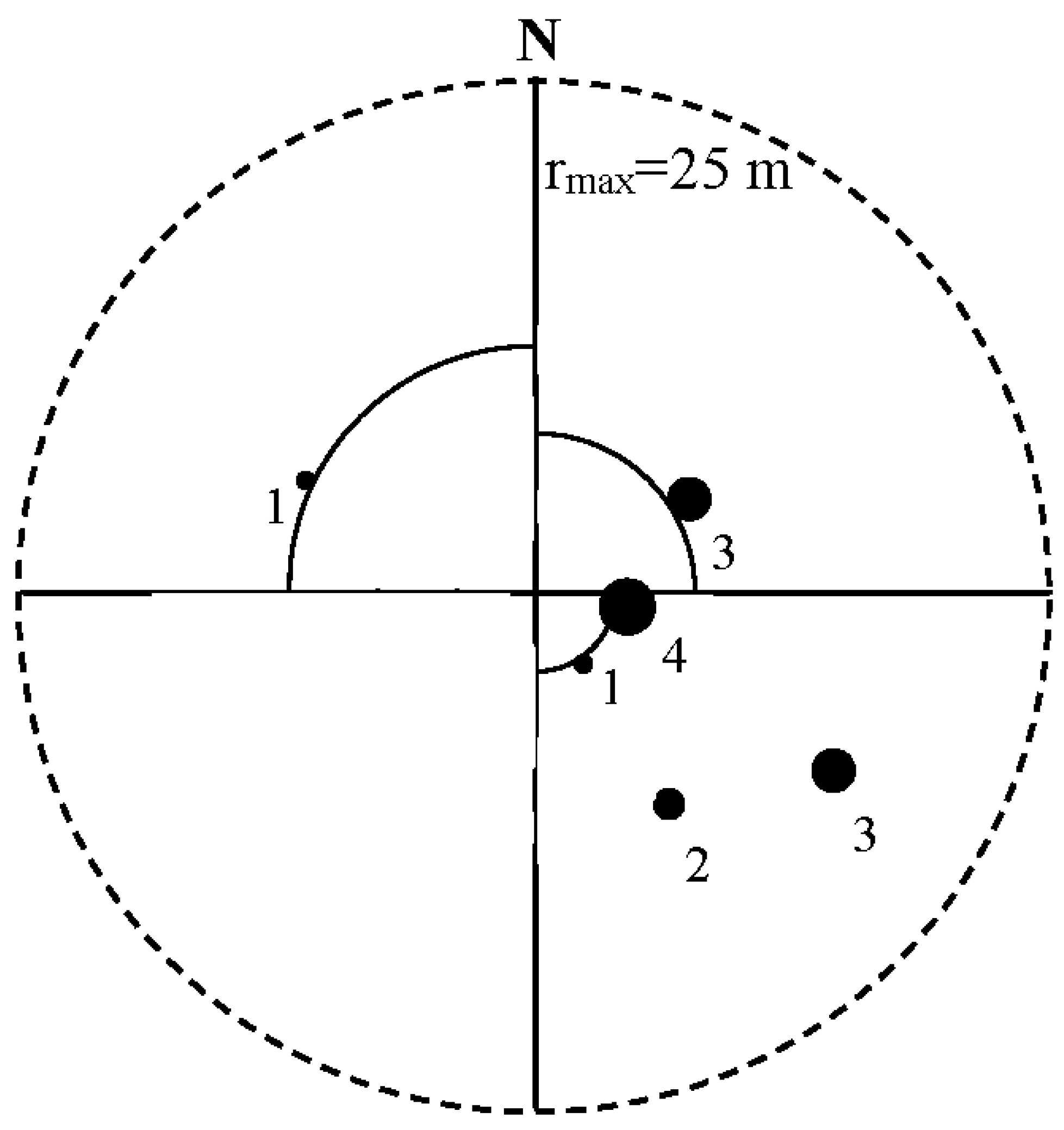
The purpose of the fieldwork was to select and georeference trees and non-tree objects that could be used as ground data for the analysis. The first field campaign was carried out in the period of 23–30 August 2006. The point-centered quarter sampling method (PCQ) [37] was used in this selection. 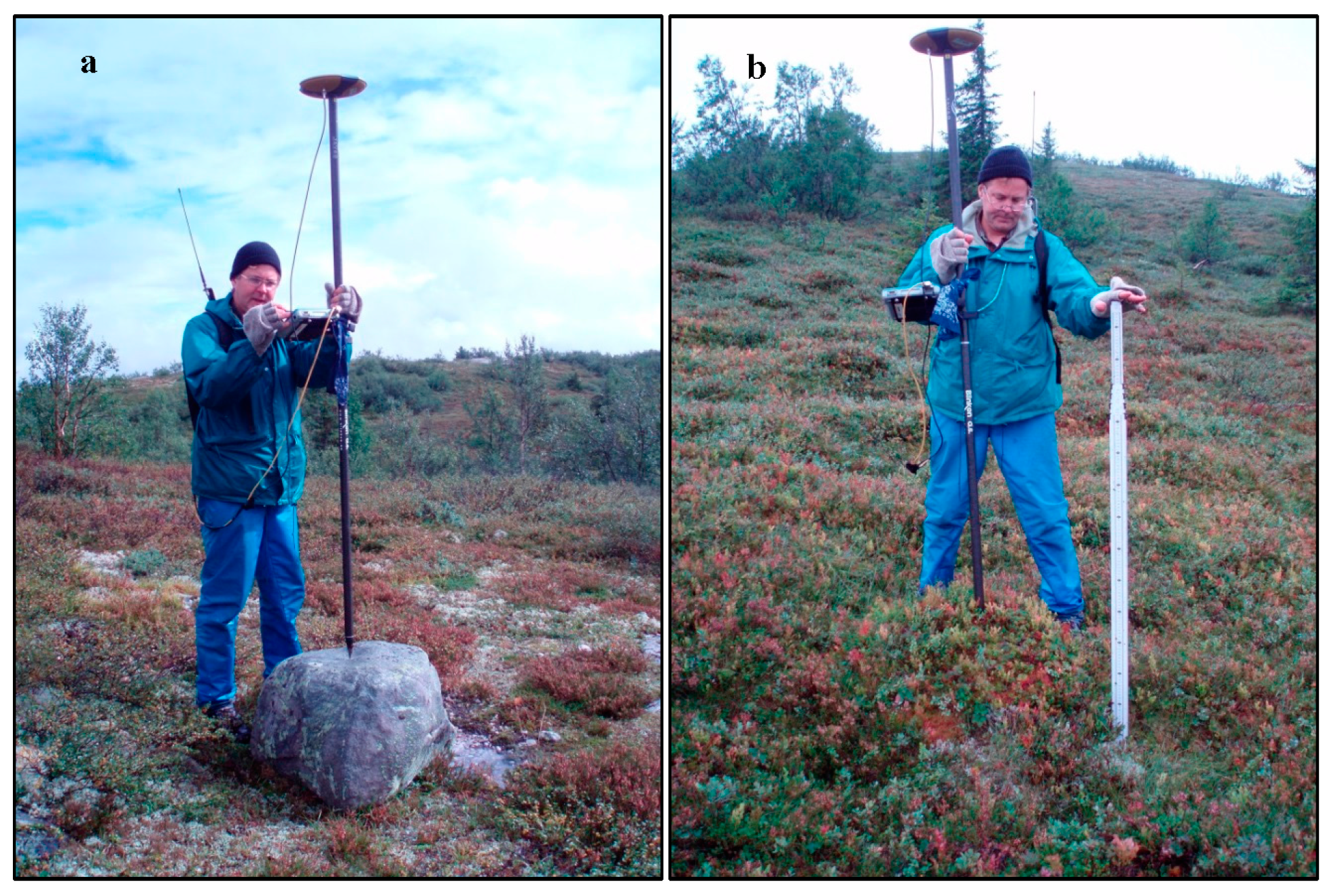Twelve pre-defined systematically distributed sample points on each of four lines with an inter-line distance of 50 m were located in field using real-time differential Global Positioning System (GPS) and Global Navigation Satellite System (GLONASS) with a local base station (Figure 1). The sample point positions and all the subsequent work to record the positions of the measured trees and other objects were determined with an expected accuracy of 3–4 cm [9]. The distance between points within each line was 50 m. These systematically distributed points were considered the sample points of the PCQ sampling. However, due to time constraints only four points were measured on line #4, see Figure 1. Thus, a total of 40 sample points were used.

For each sample point, the area around the point was divided into four quadrants according to the four cardinal directions, i.e., N-S and E-W. Within each quadrant, the closest tree to the sample point in each of four tree height classes was recorded. A maximum search distance of 25 m was used. The four tree height classes that were used were: (1) <1 m; (2) 1–2 m; (3) 2–3 m; and (4) >3 m. In addition to the trees selected by PCQ sampling, 14 trees were purposefully selected to cover gaps in the dataset. For each tree, stem position, tree species, tree height, stem diameter at root collar, and crown diameter in two perpendicular directions (N-S and E-W) were recorded. Average crown diameter was computed as the mean value of the two measurements. In total, 341 trees were selected, i.e., 121 Norway spruce, 60 Scots pine, and 160 mountain birch trees with tree heights ranging between 0.11 and 5.20 m (

Table 1. Summary of field measurements of trees.

Tree Species	Characteristic	n	Range	Mean
	Tree height (m)	121	0.25–5.20	1.75
Norway spruce	Stem diameter 1 (cm)	121	1.00–20.4	5.95
	Crown diameter (m)	121	0.21–4.30	1.41
	Tree height (m)	60	0.11–1.60	0.41
Scots pine	Stem diameter 1 (cm)	60	0.50–5.50	1.46
	Crown diameter (m)	60	0.05–1.03	0.35
	Tree height (m)	160	0.24–4.08	1.54
Mountain birch	Stem diameter 1 (cm)	160	0.90–16.3	4.00
	Crown diameter (m)	160	0.15–3.75	1.26

¹ Stem diameter at root collar.

).

A similar procedure was used to select non-tree objects. In each of the four quadrants associated with each sample point, the closest non-tree object was selected in each of the four height classes. However, due to time constraints during fieldwork in 2006, such objects were only selected along sample line #1 (Figure 1). The dataset was therefore complemented with measurements of non-tree objects on the remaining lines #2–#4 in 2010. The fieldwork in 2010 took place on 11–12 August. Because non-tree objects (tussocks, hummocks, and boulders; see details below) are fairly stable over such short time periods (four years), splitting the data collection on two seasons is not expected to have any impact on the results.

The selected objects were georeferenced, and the height and width were measured in a similar way as for the trees. These objects were classified into two categories: (1) objects with a surface of organic material like tussocks, hummocks, and rocks covered with moss and other vegetation; and (2) bare rock and boulders (Figure 2). A total of 159 non-tree objects were measured, i.e., 61 rocks and 98 with organic surface. None of these objects were taller than 1.1 m (

Table 2. Summary of field measurements of non-tree objects.

Tree Species	Characteristic	n	Range	Mean
Organic material 1	Height (m)	98	0.10–0.50	0.23
	Object diameter (m)	98	0.30–1.50	0.67
Rock	Height (m)	61	0.12–1.10	0.36
	Object diameter (m)	61	0.30–2.65	0.74

¹ Tussocks, hummocks, and rocks covered with moss and other vegetation.

).

2.3. Laser Data Acquisition

Laser scanner data were acquired under leaf-on conditions on two occasions. The first acquisition took place 24 July 2006 using the Optech ALTM 3100C laser scanner system [9]. In the present study this sensor was denoted as “ALTM 3100C”. Average flying altitude was 700 m above ground level and the pulse repetition frequency (PRF) was 100 kHz. For convenience, this acquisition was designated ACQ₁.

The three other ALS data acquisitions were carried out 11 June 2007 [16,34]. The instrument used in 2007 was an upgraded version of the Optech ALTM 3100C used in 2006. After upgrade, the system had dual pulse capabilities, which implies that it was capable of handling two pulses in the air at a time. In this study, it was denoted as “ALTM Gemini”. It should be noticed that sensor-specific properties such as pulse width, pulse energy, and peak power were altered during upgrade (

Table 3. Summary of laser scanner data and flight parameters of the four laser data acquisitions.

Parameter	Acquisition
	ACQ1	ACQ2	ACQ3	ACQ4
System	ALTM 3100C	ALTM Gemini	ALTM Gemini	ALTM Gemini
Pulse width	14.7 ns	>14.7 ns 1	2	2
Pulse energy	69 μJ	<69 μJ 1	2	2
Peak power	4.7 kW	<4.7 kW 1	2	2
Wavelength	1064 nm	1064 nm	1064 nm	1064 nm
Repetition frequency	100 kHz	125 kHz	166 kHz	166 kHz
Scan frequency	70 Hz	70 Hz	70 Hz	70 Hz
Pulse mode	Single	Single	Single	Dual
Date	24 July 2006	11 June 2007	11 June 2007	11 June 2007
Mean flying altitude 3	700 m a.g.l.	700 m a.g.l.	700 m a.g.l.	1130 m a.g.l.
Flight speed	80 m∙s−1	75 m∙s−1	75 m∙s−1	75 m∙s−1
Max. scan angle	14°	14°	14°	10°
Max processing angle	14°	14°	14°	10°
Mean footprint diameter	18 cm	17 cm	17 cm	28 cm
Point density first-of-many and single echoes	7.7 m−2	9.1 m−2	11.0 m−2	8.4 m−2

¹ Specific values not released by Optech Inc. However, the ALTM 3100C and the ALTM Gemini are the same instruments before and after upgrade, respectively. Thus, assumptions about the pulse properties can be drawn on the basis of the change in repetition frequency. ² Instrument specifications were not released by Optech Inc., however, pulse width will be larger than pulse width of the 125 kHz acquisition (ACQ₂), whereas pulse energy and peak power will be lower. ³ a.g.l. = above ground level.

).

When planning the 2007 acquisitions, the objective was to fly the sensor in such a way that it would be possible to: (1) compare acquisitions between sensors with sensor and flight properties as similar as possible (sensor comparison); (2) compare pulse repetition frequencies; and (3) compare flying altitudes. All the four ALS datasets were, therefore, acquired by flying along two northeast/southwest oriented and parallel flight lines each time. The coordinates of the flight lines were as similar in the four acquisitions as practically feasible.

The major purpose of the ALS acquisitions was to study vegetation, primarily small pioneer trees. The operating parameters of the aircraft and instruments were determined for this purpose. A preliminary investigation in another study area with mature forest indicated that the best correspondence between canopy height distributions derived from the ALTM 3100C data at 100 kHz and from the ALTM Gemini could be obtained by flying the ALTM Gemini system with a 125 kHz PRF. The first of the 2007 acquisitions was, therefore, carried out with an average flying altitude of 700 m above ground level and a 125 kHz PRF. This acquisition was designated ACQ₂ and it was intended for comparisons of sensors (ALTM 3100C vs. ALTM Gemini) and pulse repetition frequencies (125 vs. 166 kHz).

Secondly, the ALTM Gemini sensor was flown at 700 m above ground level with a 166 kHz PRF, designated ACQ₃. This acquisition allowed comparisons of pulse repetition frequencies (125 vs. 166 kHz) and flying altitudes (700 vs. 1130 m above ground level). Finally, ALTM Gemini was flown at 1130 m above ground level at a PRF of 166 kHz, designated ACQ₄, and it allowed comparison of flying altitudes (700 vs. 1130 m above ground level). It should be noted that dual pulse mode was required to capture data at 1130 m with 166 kHz (ACQ₄).

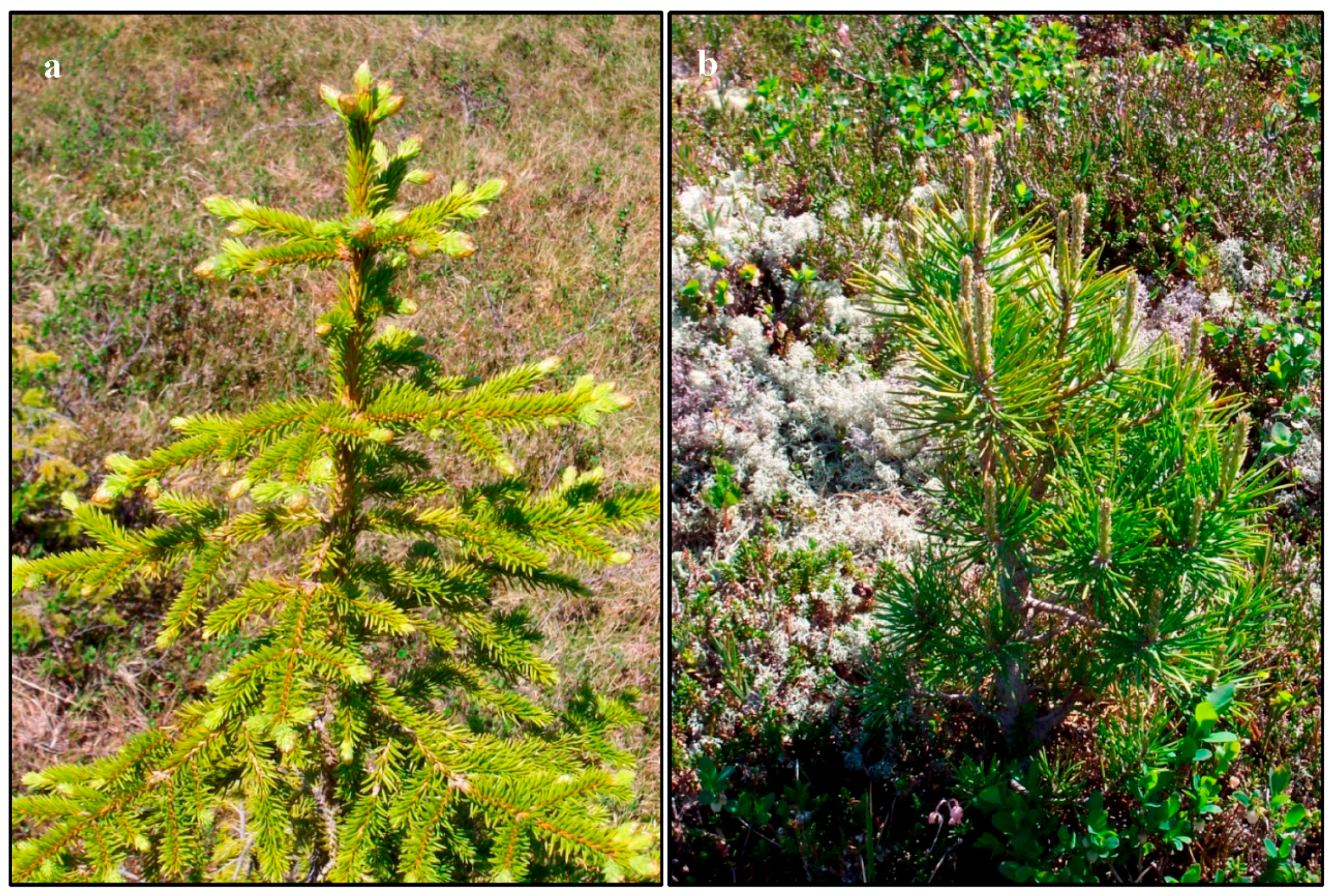
Seasonality will influence structure and color of the vegetation and may as a result affect the laser backscatter signal. A basic requirement for the comparison of sensors was that the trees and other ground vegetation were in a similar state on 24 July 2006 when the ALTM 3100C data were acquired and on 11 June 2007 when the ALTM Gemini data were acquired. In late July, the ground vegetation can be expected to be fully developed and the tree growth has normally terminated. In early to mid-June, the tree growth and state of the ground vegetation is subject to large inter-annual variations, depending on snow conditions and temperature. It was important to have full control over the conditions when the second acquisition took place in 2007. A field visit therefore took place at 11:00 a.m. UTC on 10 June 2007—28 h before the ALTM Gemini acquisitions took place (3:20 p.m.–3:55 p.m. UTC on 11 June 2007). Across the entire study area it appeared that heather and small bushes like dwarf birch (Betula nana) and willow tickets (various Salix species) were fully developed (Figure 3). So was also the grass, apart from a few wet spots where the snow had melted recently and dead grass from the previous year was still visible. The buds had just started to burst on the spruce trees (Figure 4). Both the birch and pine trees were in a similar stage of development.

2.4. Laser Data Processing

The laser data were pre-processed by the contractor (Blom Geomatics, Oslo, Norway). Planimetric coordinates (x and y) and ellipsoidic height values were computed for all laser points. Since each of the four ALS acquisitions consisted of two overlapping strips, a strip adjustment was carried out by the contractor using TerraMatch software [38]. The strip-wise elevation was corrected by a constant factor ranging from −0.130 m to +0.166 m for the individual strips [39]. The maximum correction difference between the two strips of an acquisition was 0.109 m (ACQ₄). In the strip adjustment, a constant strip-wise roll correction of 0.0023–0.0080 degrees was also applied.

The laser points used to derive terrain models were the echoes labeled “last-of-many” and “single”. Because of the generally low vegetation in the study area, most of the echoes were of the type “single”. For each of the four ALS acquisitions, TerraScan software [40] was used to classify ground points and derive terrain models. Triangulated irregular networks (TINs) were then generated for the four ALS acquisitions using the planimetric coordinates and corresponding height values of the “last-of-many” and “single” echoes classified as terrain ground points according to the progressive triangular irregular network densification algorithm [41] of TerraScan. The classification of ground points to obtain the four different TIN models was based on typical parameters used in operational projects. The “iteration distance” [40] was set to 1.0 m. The other major parameter controlling the outcome of the classification, i.e., the “iteration angle” was assigned a value of nine degrees. Further details regarding the terrain modeling can be found in [34].

After having constructed the terrain models, all “first” echoes, which contained the aggregated data of the echoes labeled as “first-of-many” and “single”, were projected onto the four different TIN surfaces and the terrain height values at these locations were computed by bi-linear interpolation. The height values of the first echoes relative to the interpolated terrain surface were computed as the difference between the echo heights and the interpolated height values at the corresponding locations on the TIN surface. These echoes along with their height values relative to the respective TIN surfaces and the raw backscatter intensity values recorded by the ALS sensors were stored and used in the subsequent analysis. The backscatter intensity as recorded by the current Optech sensors is a unit-less quantity captured in 12-bit dynamic measurement range. The point density of the first echoes for the different acquisitions ranged between 7.7 and 11.0 points m⁻² (Table 3).

The raw backscatter intensity values (I_raw) were range-normalized prior to analysis using the equation

$$I=I_{\mathrm{raw}}{\left(\frac{R}{R_{\mathrm{ref}}}\right)}^a$$

(1)

where I is the range-normalized intensities, R is the range from the sensor to the target, and R_ref is the reference range that was set equal to the mean flying altitude (Table 3). The value for the parameter a was set equal to 2 [42,43].

During data inspection, two anomalies were identified for acquisitions ACQ₃ and ACQ₁. First, it was noticed that the eastern strip of ACQ₃ had significantly higher intensity values than the western strip. It was revealed that data were collected along the eastern strip at a PRF of 142 kHz rather than the planned PRF of 166 kHz, which was used for the western strip. This difference in PRF was caused by an automatic and uncontrolled PRF shift for the eastern strip due to dual pulse mode that was induced as the aircraft passed over low terrain and approached the study area located at a higher altitude. The increasing terrain elevation as the aircraft came in from a northeastern direction is indicated by the contour lines in the map (Figure 1). The automatic shift in PRF is implemented to avoid a risk of losing data when there is a rapid decrease in distance between the aircraft and the ground. A thorough description of this effect and its influence on the specific dataset is provided in [34] along with a graphical illustration of the phenomenon. Rather than accounting for the differences in PRF for the two strips of ACQ₃ in the subsequent analysis, which would complicate the analysis (see e.g., [34]), we decided to use a simple ratio estimator to correct the range-normalized intensities prior to analysis. For the 217,698 laser points of the eastern strip located within the circular sample plots (Figure 1) and the 647,365 points of the western strip in the plots, the ratio of the mean intensity of the western strip divided by the mean of the eastern strip was calculated, and this ratio (0.778) was used to correct (multiply) every individual range-normalized intensity value along the eastern strip.

Second, it was revealed that ACQ₁ was subject to so-called banding effect. Banding is caused by differences in intensity between scan directions of the oscillating mirror, i.e., between the positive and negative scan directions. The particular ALTM 3100C instrument used in this study (serial no. 05SEN180) is known to have this banding effect for acquisitions that were carried out in 2006. After the 2006 season, this particular instrument was upgrade to ALTM Gemini and the banding effect was markedly reduced [44].

During summer of 2006, ALTM 3100C (serial no. 05SEN180) was used to collect data in Finland and Norway for more than 15 published scientific studies of which at least seven dealt with in-depth analyses of backscatter intensity. Only one of them acknowledged and adjusted for the banding effect [45]. Many of the studies related to backscatter intensity advocate the necessity of range normalization. To indicate the relative impact of banding correction vs. range normalization on the corrected intensity values, the 532,205 laser points of ACQ₁ that hit within the circular sample plots were analyzed. The mean range-normalized intensity of the negative scan direction (269,205 points) was 81.16 while for the positive direction (263,000 points) it was 88.36, a difference of 7.2. In comparison, the effect of the range normalization (compared to raw intensity values) was a mean change (absolute values) in intensity of 7.56. Clearly, the order of magnitude was very similar for the banding effect and the range normalization. However, while range normalization will help reducing variability in intensity caused by range differences from point to point, the banding is a systematic effect (between-scan variation) which is manifested as a higher variability in the data if not accounted for. In the current study, a simple ratio estimator was applied to account even for the banding effect. The mean range-normalized intensity of the positive scan direction was divided by the mean intensity of the negative direction, and this ratio (1.089) was used to correct (multiply) every individual value of the negative direction of ACQ₁. We also verified empirically that there was no banding effect present in the 2007 datasets (ACQ₂–ACQ₄). Details on the banding effect for the particular ALTM 3100C instrument can be found in [45].

2.5. Computations and Analysis

A first step in identification of small trees in the boreal-alpine ecotone would be to consider laser echoes with height (h) > 0 as candidate echoes for tree hits because positive height values is the only indication there is of presence of objects above the terrain surface. Thus, in this study, the analysis was based only on those echoes with h > 0. The analysis may take two different approaches: (1) assume that adjacent echoes (clusters) with h > 0 are objects that could be targeted and thus base the analysis on intensity properties of such individual objects; or (2) consider each echo as an individual observation in the analysis. In this study, the first approach was taken to address Objectives A and B and the latter approach was taken to address Objective C.

2.5.1. Analysis of Objects—Objectives A and B

Multiple logistic regression analysis was used to model the probability of laser echoes being reflections of a tree. First, the probability was modeled based on individual objects as observations in the analysis. Thus, rather than using clustering based on the ALS data themselves, the outlines of the trees and non-tree objects were used as they were identified in field according to position and width. As opposed to clustering or segmentation based on the ALS data, e.g., [36], which would introduce errors in the reference objects of the study (trees and non-tree objects), use of the true objects as they were identified in field offered an opportunity to study the intensity properties of the objects in question minimizing the uncertainty of what object the laser pulses actually were reflected from. We therefore started by considering each field-recorded object (trees and non-trees) as a circular object with the mean of the N-S and E-W diameter recordings (see above) as the diameter of the circle. The laser measurements where then extracted for these circles and these measurements were subject to analysis.

The mean range-normalized intensity of all echoes within an object with h > 0 was applied as an explanatory variable (${\overline{I}}_{h>0}$). Because some objects will consist of only a solitary echo, as seen also in the current dataset, candidate intensity metrics must be such that they are defined even when only one individual echo is present. Metrics like standard deviation and coefficient of variation were therefore not considered even though they have been among the metrics suggested in tree species classification of larger trees (e.g., [27]). For small trees, it is likely that some of the echoes with h > 0 will be ground hits not classified as such because of ALS measurement errors, ground classification errors, and the general uncertainty of the modeled terrain surface [34]. The most reliable echo of an object in the sense that it has the highest probability of actually being an echo belonging to an object not being part of the terrain is the echo with the highest height value (h_max). Thus, it is likely that the intensity of this echo has a value that to a larger extent than echoes closer to the ground captures the reflectivity properties of the object in question. The intensity of the echo with the largest height value within an object ($I_{h_{\max }>0}$) was therefore introduced as an explanatory variable in the analysis. Thus, the probability of an object being a tree (${\pi }_{\mathrm{TREE}}$) was modeled according to a logistic regression model with binary response and two explanatory variables, i.e., ${\overline{I}}_{h>0}$ and $I_{h_{\max }>0}$:

$$\log \left(\frac{{\pi }_{\mathrm{TREE}}}{1-{\pi }_{\mathrm{TREE}}}\right)=\mathsf{\alpha }+{\mathsf{\beta }}_1{\overline{I}}_{h>0}+{\mathsf{\beta }}_2{I}_{h_{\max }>0}$$

(2)

Maximum-likelihood computation for fitting of the logistic model in Equation (2) was performed with the logistic regression procedure of the SAS statistical software package [46]. The Hosmer–Lemeshow statistic [47] was used to assess the model fit. Separate models were fitted for each of the four ALS acquisitions.

The fitted logistic regression models were also assessed by leave-one-out cross validation. For each of the four models, one of the observations was removed from the dataset at a time, and the model was fitted to the data from the remaining observations. The probability of an object being a tree was predicted according to Equation (3):

$${\pi }_{\mathrm{TREE}}\text{=}\frac{\exp \left(\mathsf{\alpha }+{\mathsf{\beta }}_1{\overline{I}}_{h>0}+{\mathsf{\beta }}_2{I}_{h_{\max }>0}\right)}{1+\exp \left(\mathsf{\alpha }+{\mathsf{\beta }}_1{\overline{I}}_{h>0}+{\mathsf{\beta }}_2{I}_{h_{\max }>0}\right)}$$

(3)

The assignment of a unique outcome for each predicted probability was done according to a deterministic approach, i.e., if the predicted probability was greater than 0.5, the object in question was classified as TREE. Classification error matrices from the cross validation of the four models were constructed, and several descriptive statistics were estimated to evaluate the performance of the regression models. First, the overall agreement was assessed by the Kappa coefficient (Κ) [48] and the agreement within the individual categories by conditional Kappa (Κ_c) [49]. These estimators have become widely used in remote sensing [50]. Κ and Κ_c quantify the relationship of beyond chance agreement to expected disagreement. The estimators of Κ and Κ_c are frequently multiplied by 100 to give percentage measures of classification accuracy. In this study, we restricted the estimation of conditional Kappa to the producer’s approach (based on errors by omission). The hypothesis, H₀: Κ = 0, was tested [49]. The hypothesis that Κ_c was 0, was tested for each of the two categories [49]. Due to the fact that two tests were performed simultaneously, the significance level in each test was set to α/(2 × 2) to control the total Type I Error (Bonferroni approach) [51].

A preliminary assessment of the intensity values indicated that the intensities of the trees tended to be lower than the intensities for some of the non-tree objects. This was particularly the case for organic material (tussocks, hummocks, and rocks covered with moss and other vegetation). At the same time, the intensities of the trees tended to be higher than the intensities of rocks. Thus, a binary response may have some problems with discriminating between trees and non-tree objects as such. It was therefore assessed to what extent the intensity values could assist in discriminating between the five basic object categories. Multinomial logistic regression analysis assuming nominal categories, i.e., unordered categories, was used to model the probability of laser echoes being reflections of spruce, pine, birch, organic material, and rocks, respectively. In the analysis, the same intensity variables as used in the model in Equation (2) were applied as explanatory variables. In multinomial logistic regression, the probabilities are jointly modeled as one system. There is one model less than there are categories. In the modeling, the probability of each category is modeled relative to the probability of a chosen baseline category. In the modeling, SPRUCE was chosen as the baseline category. Thus, for the k categories PINE, BIRCH, ORGANIC, and ROCK, the probabilities of category j (${\pi }_{\mathrm{PINE}}$, ${\pi }_{\mathrm{BIRCH}},$ ${\pi }_{\mathrm{ORGANIC}}$, and ${\pi }_{\mathrm{ROCK}}$) were modeled according to the following multinomial logistic regression model:

$$\log \left(\frac{{\pi }_j}{1-{\pi }_{\mathrm{SPRUCE}}}\right)={\mathsf{\alpha }}_j+{\mathsf{\beta }}_{1j}{\overline{I}}_{h>0}+{\mathsf{\beta }}_{2j}{I}_{h_{\max }>0}$$

(4)

Maximum-likelihood computation was applied for fitting the model in Equation (4). The logistic regression procedure of the SAS statistical software package [46] was used. Separate models were fitted for each of the four acquisitions. There is no obvious choice for a single goodness-of-fit statistic for the multinomial case, although some tests have been proposed lately, e.g., [52,53]. In this study, deviance and Pearson chi-square goodness-of-fit statistics are reported.

These regression models were also assessed by leave-one-out cross validation. The cross validation was carried out according to the same procedure as described for the binary case above. In the multinomial case, the probabilities of the five mutually exclusive outcomes were predicted according to

$${\pi }_{j }\text{=}\frac{\exp \left({\mathsf{\alpha }}_j+{\mathsf{\beta }}_{1j}{\overline{I}}_{h>0}+{\mathsf{\beta }}_{2j}{I}_{h_{\max }>0}\right)}{1+{{\displaystyle \sum }}_k\exp \left({\mathsf{\alpha }}_k+{\mathsf{\beta }}_{1k}{\overline{I}}_{h>0}+{\mathsf{\beta }}_{2k}{I}_{h_{\max }>0}\right)}$$

(5)

for the k non-baseline categories PINE, BIRCH, ORGANIC, and ROCK, and according to Equation (6) for the baseline category (SPRUCE), i.e.,

$${\pi }_{\mathrm{SPRUCE} }\text{=}\frac{1}{1+{{\displaystyle \sum }}_k\exp \left({\mathsf{\alpha }}_k+{\mathsf{\beta }}_{1k}{\overline{I}}_{h>0}+{\mathsf{\beta }}_{2k}{I}_{h_{\max }>0}\right)}$$

(6)

The assignment of a unique outcome for each object was done according to a deterministic approach. In the multinomial case the assignment was done by choosing the outcome with the highest predicted probability among the five categories. For each of the four resulting error matrices, the overall and conditional (producer’s approach) Kappa coefficients were estimated (see above). It was tested for statistical significance of Κ and Κ_c as described above. The level of significance in the tests performed for Κ_c was α/(2 × 5).

To address Objective A, i.e., to evaluate if classification into individual tree species (SPRUCE, PINE, BIRCH) and individual types of non-tree objects (ORGANIC, ROCK) could improve the overall performance of a binary tree/non-tree classification, the classification into five categories was aggregated to two categories. These aggregated 2 × 2 error matrices were then compared to the error matrices resulting from the binary case. The comparison was based on Κ. Thus, the one-sided hypothesis H₀: Κ_multinomial > Κ_binary [54] where Κ_multinomial is the overall Kappa of the aggregated 2 × 2 error matrix from the multinomial case and Κ_binary is the overall Kappa of the binary case was tested.

Finally, to address Objective B, the overall classification agreement obtained when aggregating the five categories to two categories was compared for different sensor and flight configurations. Pairwise comparisons were performed for: (1) ACQ₁ against ACQ₂ (effect of sensor); (2) ACQ₂ against ACQ₃ (effect of PRF); and (3) ACQ₃ against ACQ₄ (effect of flying altitude). Thus, in each comparison, the hypothesis H₀: Κ_i − Κ_j,j≠i = 0 was tested. Since three tests were performed simultaneously, the level of significance in each test was set to α/(2 × 3) (two-sided tests, Bonferroni approach).

2.5.2. Analysis of Individual Echoes—Objective C

An analysis was also conducted with individual echoes as unique observations in the analysis rather than using clusters of echoes (objects). In an operational case of tree identification in the boreal-alpine ecotone based on ALS data, a large portion of echoes with h > 0 will be reflections from non-tree objects like tussocks, hummocks, rocks, and other structures on the terrain surface, although the magnitude of such echoes will depend on surface morphology, algorithms and parameters used to derive the terrain model from the ALS data, and other factors. However, in the ecotone in question the tree density will normally be low with large distances between adjacent trees. Thus, the relative number of echoes with h > 0 assigned to trees will be low compared to the total number of echoes with h > 0. To mimic a situation with relatively large areas without trees, the basic properties of the PCQ sampling design was utilized, i.e., the fact that within each quadrant the closest tree to the sample point is always selected as a sample tree. For each of those quadrants that contained at least one tree recorded in field, the nearest tree to the sample point was identified. All echoes with h > 0 within a sector restricted by the N-S and E-W axes through the sample point and the periphery of a quarter circle touching the crown polygon of the closest tree were extracted (Figure 5). These echoes were considered as non-tree echoes. For these sectors one could be sure that there were no other trees. However, in certain cases it may happen that the crown of the second closest tree to the sample point or the crown of a tree located close to a neighboring quadrant has parts of its crown inside the sector of the closest tree to the sample point in a given quadrant (see the tree in the fourth height class in the SE quadrant in Figure 5 for an illustration). The laser echoes within the crown polygons of such adjacent trees were removed. Furthermore, manual inspection of orthophotos revealed that for some of the sectors that satisfied the criterion for being included in this analysis, there were trees located just outside the quarter circle that were not recorded in field but had parts of their crows inside the relevant sectors. This happened when such trees belonged to the same height class as the closest tree and thus were not subject to field measurements according to the sampling protocol. Whenever this happened, the entire sector in question was discarded from the analysis since it was not possible to control the extension of these non-recorded trees. Thus, 24 sectors were discarded and the subsequent analysis was based on a total of 136 sectors. It should be noted though, that for these sectors the trees themselves did not necessarily have to be hit by any laser pulses for the sectors to be included in the analysis.

First, logistic regression analysis was used to model the probability of laser echoes being reflections of a tree (${\pi }_{\mathrm{TREE}}$) using the height of the individual echoes (h_h>0) as the only explanatory variable. Separate models were estimated for the different acquisitions. These models were fitted with binary response and one explanatory variable, i.e., h_h>0, following the estimation procedure applied for Equation (2) above:

$$\log \left(\frac{{\pi }_{\mathrm{TREE}}}{1-{\pi }_{\mathrm{TREE}}}\right)=\mathsf{\alpha }+{\mathsf{\beta }}_1{h}_{h>0}$$

(7)

These models were cross validated by leave-one-out cross validation following the procedure outlined above. The results of the cross validation was considered as “benchmark” for validation of a more sophisticated model which also included the intensity as explanatory variable. Thus, a second set of models were fitted with the intensity of echoes with h > 0 (I_h>0) as an additional variable in the analysis:

$$\log \left(\frac{{\pi }_{\mathrm{TREE}}}{1-{\pi }_{\mathrm{TREE}}}\right)=\mathsf{\alpha }+{\mathsf{\beta }}_1{h}_{h>0}+{\mathsf{\beta }}_2{I}_{h>0}$$

(8)

These models were also cross validated as described above. Overall Kappa and conditional Kappa values were computed.

To address Objective C specifically, i.e., to assess the contribution of backscatter intensity data to improve classification accuracy beyond what can be obtained from using echo height it was tested if a classification based on height as well as intensity produced a higher agreement than a classification based on height only. Thus, classification error matrices were constructed from the cross validations of models fitted according to Equations (7) and (8). A pairwise comparison was conducted based on the overall Kappas. This was accomplished by testing the one-sided hypothesis H₀: Κ_h,I > Κ_h, where Κ_h,I is the overall Kappa of an error matrix resulting from validation of the model in Equation (8) and Κ_h is the overall Kappa of an error matrix resulting from validation of the model in Equation (7). Such tests were performed for the four different ALS acquisitions.

3. Results

3.1. Analysis of Objects

Large differences in intensities between the different ALS acquisitions were revealed (Figure 6). The mean values of the tree-level intensities for spruce trees ranged from 18.1 for ACQ₄ to 79.6 for ACQ₁ (

Table 4. Range-normalized intensity values for individual trees and non-tree objects (for echoes with h > 0) and for those individual echoes of each tree and non-tree object with h = h_max (h_max > 0). Only objects with at least one echo with h > 0 are included.

Acquisition	Type of Objects	No. of Objects	No. of Echoes	Intensity of Individual Objects				Intensity of Individual Echoes
				Mean		SD
				Range	Mean	Range	Mean	Mean	SD
	Spruce	104	1230	56.3–94.8	79.6	0–17.6	8.3	75.0	10.8
	Pine	7	9	69.3–106.0	84.7	5.8–7.8	6.8	84.5	13.2
ACQ1	Birch	125	1239	66.0–112.4	82.8	0–17.5	8.6	80.2	11.7
	Organic 1	43	132	68.5–123.1	91.7	0–12.6	6.1	90.0	12.3
	Rock	41	143	53.7–108.6	75.3	0–24.8	10.9	73.9	17.7
	Spruce	103	1702	19.9–37.2	30.0	0–14.2	3.0	28.2	4.6
	Pine	15	23	27.3–36.1	31.9	0.5–5.3	2.0	31.6	2.3
ACQ2	Birch	137	1614	21.6–38.6	29.2	0–7.0	2.9	27.0	5.2
	Organic 1	70	210	24.0–39.8	32.8	0–9.0	1.8	32.6	3.7
	Rock	42	199	20.5–38.1	27.6	0.9–5.8	3.1	27.6	5.4
	Spruce	110	2372	15.1–21.9	18.3	0.5–3.8	2.0	17.0	2.7
	Pine	23	44	14.3–24.4	18.2	0.6–4.0	2.0	17.8	3.1
ACQ3	Birch	142	2442	14.0–23.6	17.9	0–4.8	2.0	16.6	3.0
	Organic 1	74	261	13.0–24.8	19.5	0–4.6	1.6	19.8	2.5
	Rock	43	255	11.8–23.5	16.6	0–4.5	1.8	16.2	2.6
	Spruce	106	1689	14.2–23.0	18.1	0–4.1	2.2	16.8	3.2
	Pine	21	31	11.5–21.1	18.0	1.3–4.7	2.7	17.9	2.9
ACQ4	Birch	134	1514	12.9–26.0	17.7	0–5.4	2.1	16.9	2.9
	Organic 1	63	165	13.3–24.4	18.9	0–4.0	1.8	19.0	2.4
	Rock	44	197	12.2–21.0	16.4	0–3.6	1.8	16.3	2.7

¹ Tussocks, hummocks, and rocks covered with moss and other vegetation.

). Correspondingly, the mean intensities for pine and birch were in the ranges 18.0–84.7 and 17.7–82.8. For non-tree objects with organic surface the mean intensities ranged from 18.9 to 91.7. For rocks the range was 16.4–75.3. The differences between acquisitions in intensity values of the single echo with the largest height value within each object (h_max) followed more or less the same patterns as the mean intensity values (Table 4).

The multiple logistic regression analysis modeling the probability of laser echoes being reflections from a tree with mean intensity (${\overline{I}}_{h>0}$) and intensity of the echo with the largest height value ($I_{h_{\max }>0}$) as explanatory variables (Equation (2)), revealed a decent fit for all models (Hosmer–Lemeshow statistic: p = 0.095–0.959,

Table 5. Model fit and results of leave-one-out cross validation of the logistic regression models with binary response fitted according to Equation (2). Only objects with at least one echo with h > 0 are included.

		Model Fit 1		Κc 2 (%)
Acq.	No. of Objects	Χ2	P-Value	TREE	NON-TREE	Κ (%)
ACQ1	320	9.4	0.310	na	0.0 ns	0.0 ns
ACQ2	367	2.6	0.959	39.1 **	6.8 *	11.6 *
ACQ3	392	13.5	0.095	9.7 ns	1.9 ns	3.2 ns
ACQ4	368	11.2	0.191	1.3 ns	0.2 ns	0.3 ns

Level of significance: ns = not significant (>0.05). * <0.05. ** <0.01. na = Κ statistic not available because model did not predict any occurrences of the category in question. ¹ Hosmer–Lemeshow statistic with df = 8 [47] (p. 140). ² Producer’s approach (based on errors of omission). Bonferroni approach with α/(2 × 2).

). Higher p-values would suggest correctly specified models, while p-values below, say, 0.05 would suggest a model with inadequate fit. Cross validation of the logistic regression models showed that the models had a limited ability to classify the trees and non-tree objects correctly. The overall classification agreement expressed by the Κ statistic was in the range 0%–11.6% (Table 5). None of the estimated Κ values, apart from the largest one (11.6%), differed significantly from zero in the statistical sense. The Κ_c values for the two individual categories, i.e., TREE and NON-TREE, indicated poor agreement for both classes in most cases.

Encouraged by the fact that the different types of non-tree objects, i.e., rocks and terrain objects covered with organic material, tended to provide echoes with lower and higher average intensity values, respectively, than the trees (Figure 6), multiple logistic regression models with the same explanatory variables (${\overline{I}}_{h>0}$ and $I_{h_{\max }>0}$) but multinomial response were fitted. The p-values of 1.000 for deviance indicated a decent fit for all models while the Pearson chi-square goodness-of-fit statistic indicated a rather poor fit for most of the models (

Table 6. Model fit and results of leave-one-out cross validation of the multinomial logistic regression models fitted according to Equation (4). Only objects with at least one echo with h > 0 are included.

		Model Fit (p-Value) 1		Κc 2 (%)
Acq.	No. of Objects	Deviance	Pearson	Spruce	Pine	Birch	Organic 3	Rock	Κ (%)
ACQ1	320	1.000	<0.001	14.6 *	na	19.6 ns	11.6 ns	19.2 **	15.5 ***
ACQ2	367	1.000	0.273	−1.4 ns	na	36.1 ***	31.7 ***	21.7 **	15.6 ***
ACQ3	392	1.000	<0.001	−2.4 ns	na	32.2 **	33.8 ***	22.0 **	14.7 ***
ACQ4	368	1.000	0.032	9.5 ns	na	24.9 *	11.1 ns	27.7 ***	14.9 ***

Level of significance: ns = not significant (>0.05). * <0.05. ** <0.01. *** <0.001. na = Κ statistic not available because model did not predict any occurrences of the category in question. ¹ Deviance and Pearson chi-square goodness-of-fit statistics. ² Producer’s approach (based on errors of omission). Bonferroni approach with α/(2 × 5). ³ Tussocks, hummocks, and rocks covered with moss and other vegetation.

). As for the Hosmer–Lemeshow statistic mentioned above, a p-value below, say, 0.05 would suggest a model with inadequate fit. However, in all models except for ACQ₁, both explanatory variables were statistically significant at the 0.1% level (not shown here).

Cross validation of the multinomial logistic regression models revealed an overall classification agreement (Κ) ranging between 14.7% and 15.6% (Table 6). All the estimated Κ values indicated overall classification agreements that were significantly higher (p < 0.001) than what could be expected due to randomness. For the five individual categories (object types), the conditional classification agreement ranged from −2.4% (not significant) to 36.1% (p < 0.001). The highest classification agreement was revealed for birch trees (BIRCH) and the two types of non-tree objects.

When the results of the cross validation based on the multinomial logistic regression models with five categories (SPRUCE, PINE, BIRCH, ORGANIC, and ROCK) were compared to the validation based on logistic regressions with binary response (TREE and NON-TREE) by aggregating the five categories into two categories (Objective A), the classification agreement appeared to increase significantly (p < 0.001–0.05) using five distinct categories in the modeling. The overall agreement was 13.7–28.1 percent points higher when aggregating the five classes into two (

Table 7. Test of differences between overall Kappas (Κ) derived from classification of trees and non-tree objects in cross validation of logistic regression models based on multinomial ¹ and binary responses, respectively.

Acquisition	Κmultinomial − Κbinary (%)	Z Statistics 2
ACQ1	28.1	4.87 ***
ACQ2	13.7	1.98 *
ACQ3	25.9	3.95 ***
ACQ4	19.7	3.56 ***

Level of significance: * <0.05. *** <0.001. ¹ Classification into five categories was aggregated to two categories. ² Test of one-sided hypothesis H₀: Κ_multinomial > Κ_binary.

).

The comparison of classification agreement across pairs of acquisitions based on the cross validation of the multinomial logistic regression models aggregated to two categories (Objective B) showed differences between Kappas in the range 2.8–9.1 percent points (

Table 8. Test of differences between overall Kappas (Κ) derived from classification of trees and non-tree objects in cross validation of logistic regression models based on multinomial ¹ response for different combinations of acquisitions.

Effect	Difference	Κi − Κj (%)	Z Statistics 2
Sensor	ACQ1 − ACQ2	−3.8	0.51 ns
Pulse rep. frequency	ACQ2 − ACQ3	9.1	1.20 ns
Flying altitude	ACQ3 − ACQ4	2.8	0.35 ns

Level of significance: ns = not significant (>0.05). ¹ Classification into five categories was aggregated to two categories. ² Two-sided tests. Bonferroni approach with α/(2 × 3).

). However, none of these differences were significant in the statistical sense (p > 0.05).

3.2. Analysis of Individual Echoes

The numbers of echoes with h > 0 found within the tree-less sectors of the PCQ quadrants were much higher than the corresponding numbers of echoes for the trees associated with the same sectors, as one would expect in the boreal-alpine ecotone where only scattered trees appear in the landscape. In this dataset, roughly 1% to 5% of the echoes with h > 0 were tree hits. For example, in ACQ₃, 1207 and 86,050 echoes were tree and non-tree echoes, respectively (

Table 9. Model fit, p-values of parameter estimates, and results of leave-one-out cross validation of logistic regression models fitted according to Equation (8). The models classify echoes of trees and non-tree objects based on range-normalized intensity and height of individual echoes with h > 0 for trees and sectors of the PCQ quadrants where non-tree echoes could be identified, see Figure 5.

	No. of Echoes		Model Fit 1		p-Value of Parameter Estimates		Κc 2 (%)
Acq.	TREE	NON-TREE	Χ2	p-Value	hh>0	Ih>0	TREE	NON-TREE	Κ(%)
ACQ1	518	7085	151.3	<0.001	<0.001	<0.001	3.3 ***	25.9 ***	5.9 ***
ACQ2	686	31,272	307.3	<0.001	<0.001	<0.001	5.6 ***	34.6 ***	9.7 ***
ACQ3	1207	86,050	30.0	<0.001	<0.001	0.004	6.8 ***	51.2 ***	12.0 ***
ACQ4	655	50,327	30.3	<0.001	<0.001	<0.001	2.6 ***	29.6 ***	4.8 ***

Level of significance: *** <0.001. ¹ Hosmer–Lemeshow statistic with df = 8 [47] (p. 140). ² Producer’s approach (based on errors of omission). Bonferroni approach with α/(2 × 2).

).

The multiple logistic regression analysis modeling the probability of individual laser echoes with h > 0 being reflections from a tree with height value (h_h>0) and intensity (I_h>0) of the echoes as explanatory variables (Equation (8)) revealed a rather poor fit for all models. The Hosmer–Lemeshow statistic displayed a p-value of <0.001 for all models (Table 9). It appeared though that the parameter estimates for h_h>0 as well as for I_h>0 were highly significant (p < 0.001–0.004, Table 9). Cross validation of the models indicated that all models produced an overall classification agreement (Κ) that exceeded what could be expected due to randomness (p < 0.001), although the agreement was relatively poor (4.8%–12.0%, Table 9). The classification agreement for individual categories, i.e., for trees and non-trees, ranged between 2.6% and 6.8% (p < 0.001) and 25.9% and 51.2% (p < 0.001), respectively.

The contribution of the intensity value (I_h>0) to the overall classification performance of the logistic model in Equation (8) was assessed by comparing the overall Kappa values in the cross validation of the models fitted according to Equation (8) with corresponding values obtained by cross validation of models fitted with height (h_h>0) as the only explanatory variable (Equation (7)) (Objective C). It was revealed that the differences in estimated Κ were close to zero (p > 0.05) for all four acquisitions (

Table 10. Test of differences between overall Kappas derived from classification of trees and non-tree objects in cross validation of logistic regression models based on height and range-normalized intensity (Equation (8)) and height (Equation (7)) as explanatory variables, respectively.

Acquisition	Κh,I − Κh (%)	Z Statistics 1
ACQ1	−0.9	0.41 ns
ACQ2	0.0	0.0 ns
ACQ3	0.4	0.25 ns
ACQ4	0.3	0.17 ns

Level of significance: ns = not significant (>0.05). ¹ Test of one-sided hypothesis H₀: Κ_h,I > Κ_h.

).

4. Discussion

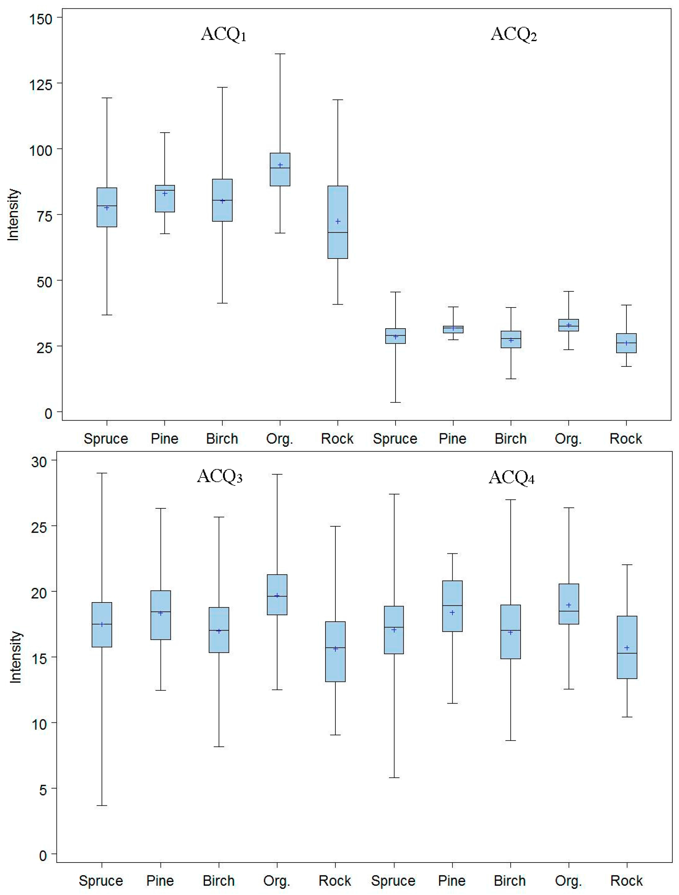
The overall finding of this study is that the range-normalized backscatter intensity of the laser echoes acquired with a 1064 nm laser has limited capacity to improve the classification of trees and non-tree objects in the boreal-alpine ecotone, although there is some evidence of differences in intensity between trees and non-trees in the statistical sense which have not been documented before.

As illustrated in this study, non-tree objects in the boreal-alpine ecotone can be vegetated as well as non-vegetated objects. Examples of vegetated objects are tussocks, hummocks, and rocks covered with moss. It is reasonable to assume that vegetated and non-vegetated objects have different reflectivity properties. The empirical findings seem to confirm that such differences exist—there is evidence of differences in backscatter intensity (Figure 6). Even different tree species will tend to produce different intensities of the reflected laser echoes. Thus, it was shown that classification into more specific classes like individual tree species and different types of non-tree objects can improve significantly the overall classification of trees and non-trees (Table 7). However, even a detailed classification into finer categories resulted in a rather poor overall classification (Κ = 14.7%–15.6%).

In the analysis of the individual echoes located in the tree-less sectors of the PCQ quadrants, it was found that backscatter intensity did not improve the overall classification (Table 10). These findings were well in line with what we found when we analyzed the laser echoes only for those objects that were identified in field. The major contribution to a successful identification of trees is the height value of the laser echoes. The height cannot discriminate between different object types, not even when the spatial patterns of the ALS echoes are taken into account [30,32], but the higher the value of an echo is the more likely is it that the echo in question comes from a tree. In some environments with abrupt topography and large rocks and boulders, the potential for erroneous classification will be high. However, in the gentle terrain found in the present study area, a high echo value was a good indicator of a tree hit. As showed in [9,31,34], almost all trees could be identified successfully when they had reached a height of around 1 m and the laser point density approached >7–8 m⁻². Thus, in many mountainous environments the problem of discriminating between trees and non-trees is basically a challenge related to the smallest trees (<1 m tall). For such trees, the intensity seems to be of little help to improve the classification. This is consistent with previous findings [30] and the more detailed classification into different tree species and different types of non-tree objects, does not change the overall picture, despite the different reflectivity properties mentioned above.

The ability to discriminate between trees and non-trees seemed to be more or less unaffected by ALS acquisition. In statistical terms there were no clear trends of different potentials for successful discrimination with different sensors, PRFs, or flying altitudes. Although one would expect acquisitions with high energy levels and narrow (precise) pulse widths of the emitted pulses to produce more consistent and less variable backscatter intensities, there were no significant differences in the statistical sense in classification agreement for the different acquisitions. However, a rather conservative test was applied (Bonferroni) and the trends indicated in Table 8 seem at least to follow a logical pattern with slightly higher agreement for the acquisition with the best pulse properties for precise measurements, i.e., ACQ₂ (cf. Table 3). It should be noted more as a curiosity that the mean backscatter intensity levels found for the small spruce, pine, and birch trees in this mountainous environment when we used the ALTM 3100C sensor (ACQ₁) corresponded very well with the intensities found for larger trees in another study. For the same three species using a similar ALTM3100 sensor with the same repetition frequency and almost the same flying altitude (750 m) over a mature forest in the lowlands Ørka et al. [55] reported mean intensities of around 80 (corrected for truncation and division by 10 which was detected after their study was published). They considered pulses with single echoes like in the present study. The average level in the current study was 79.6 (Table 4). However, these seemingly consistent values can hardly be considered as evidence of stability and robustness of ALS intensities for vegetation characterization.

The different ALS datasets analyzed in this study were acquired at two different times of the year. While ACQ₁ was acquired in late July, the other three acquisitions were accomplished in the first half of June. There are often considerable differences in phenology in the boreal-alpine ecotone at these two times of the growing season. This pertains to the trees as well as the ground vegetation. In early June, also higher moisture content in the ground vegetation and even open water bodies left after recently melted snow is normal. Although one would expect these differences in the ground vegetation to influence on reflectivity, the ability to discriminate between trees and non-trees did not seem to follow any seasonal patterns. As is evident from for example Table 6, the ability to classify trees did not differ more between the July acquisition (ACQ₁) on one hand and the three June acquisitions on the other than it differed between the three respective June acquisitions. Thus, the different dates of the ALS acquisitions do not seem to have had a significant impact on the results.

In the second part of this study, it was focused on individual echoes rather than objects. By using the echoes in the tree-less sectors of the PCQ quadrants along with the echoes of the trees associated with those sectors we got a fairly realistic distribution of number of echoes in the different categories, although it is likely that the proportion of tree echoes was somewhat higher than the true proportion because the PCQ method tend to be positively biased [56]. However, we still got about 20 to 100 times more non-tree echoes than tree echoes. Modeling can be challenging with such uneven distributions. When there is a very uneven balance between “zeros” (non-trees) and “non-zeros” (trees), one might for example consider the so-called zero-inflated models, e.g., zero-inflated Poisson models and zero-inflated negative binominal models (see e.g., [57] for an overview of these model types). Such modeling techniques were recently applied to modeling and prediction of rare trees using ALS data [58]. In such models, the “zeros” are attributed to one process, whereas “non-zeros” are attributed to another process. Thus, the two processes are specified differently. Although the “non-zero” process is usually expected to have several outcomes, zero-inflated models have also been used for processes with binary response [59]. Since establishment of new trees in the boreal-alpine ecotone is governed partly by environmental factors related to for example wind speed, wind direction, and snow-cover, modeling of the “non-zeros” process could perhaps benefit from including variables such as slope and aspect. It was nevertheless beyond the scope of the current study to address variables beyond backscatter intensity since they were studied in [30,32].

Several aspects of the applied laser systems and the treatment of the backscatter intensity recordings may be worth mentioning. First, the sensors used in the current study operate at 1064 nm (Table 3), which is a commonly used wavelength of proprietary laser scanners for terrestrial applications. Although previous studies have indicated some discriminating power at this wavelength in similar vegetation environments [28], other wavelengths may be more suitable as suggested by spectral libraries (e.g., http://pubs.usgs.gov/of/2003/ofr-03-395/datatable.html). Multispectral laser systems, which are about to emerge in the propriety domain, may provide additional opportunities for use of backscatter intensity for classification of vegetation. This was also demonstrated by Morsdorf et al. [60]. Second, we have no information on the proprietary methods for deriving the intensity values. This, along with other sensor properties, is usually considered confidential information [33] and can in fact be a major limitation of using intensity information. Third, simple range normalization was undertaken in the current analysis. More sophisticated means, such as normalization based on the reflectivity properties of the target objects, could potentially improve the discriminating power of the backscatter intensity. Finally, laser intensity values may be affected by the so-called edge effect [61] occurring on the edge of an object where the laser beam is split. This results in either an attenuated laser intensity value or a laser intensity value that is actually reflected from at least two objects [62]. The footprint sizes in the current study are 17–28 cm (Table 3). Thus, attenuated laser intensity values are the most likely result on trees in the boreal-alpine ecotone. Most of the small trees located in this ecotone feature small-sized leaves that provide a longer duration of return energy to the sensor and lower intensity than for solid objects without edges within the footprint.

Regardless of the discriminating power of backscatter intensity, there is clearly a lower limit in terms of tree sizes that possibly can be detected by ALS. Since echo height is the strongest indicator of objects with a vertical extension above the terrain surface, the accuracy of the digital terrain model may give an indication of trees that may be detected. In a recent study of terrain model quality based on data from the current study area [16], it was concluded that 0.15–0.30 m in height seems to remain a lower bound on tree sizes that one potentially can expect to detect under ideal conditions. However, as long as discrimination between different types of objects remains a challenge, the knowledge of the presence of objects with sizes down to 0.15–0.30 m in height is less useful for tree identification.

Nevertheless, for monitoring of changes in particular, as opposed to inventory, Næsset and Nelson [9] pointed out that ALS can be considered a sampling device when making multi-temporal measurements of small trees over time. Thus, objects that remain stable over time, like rocks and convex terrain structures that would be considered as potential sources of commission errors in inventory will have less influence on change estimates. Although some non-tree objects appearing in a first acquisition will not be hit in a second acquisition and vice versa since pulse placement on the ground will change between acquisitions, such changes will balance out for a given target area with large sample sizes. A successful detection of for example migration of the tree line therefore does not rely on a perfect classification of trees/non-trees as long as the height measurements are reliable and well calibrated at each point of time [34]. Hence, low echoes close to the modeled terrain surface may still carry useful information for monitoring purposes even if classification of the actual object is difficult.

5. Conclusions

This study has shown that backscatter intensity of ALS is hardly of any use in classification of small trees and non-trees in the boreal-alpine ecotone. The most essential variable for identifying the trees is the ALS height measurement. Because heights greater than, say, 1 m in most mountainous environments is a good indication of a tree, most trees can be detected when they are taller than around 1 m, provided that the laser point density is fairly high (>7–8 m⁻²) [9,31,34]. Even though low pulse repetition frequencies enable high energy levels and narrow pulse widths with higher measurement precision than higher repetition frequencies, no differences in the ability to discriminate between trees and non-trees could be found between pulse repetition frequencies, sensors, and flying altitudes. For monitoring purposes in particular, low echoes close to the modeled terrain surface may nevertheless still carry useful information even if classification of the actual object is difficult or even impossible.