Article

Improving Streamflow Prediction Using Remotely-Sensed Soil Moisture and Snow Depth

1
State Key Laboratory of Hydrology-Water Resources and Hydraulic Engineering, College of Hydrology and Water Resources, Hohai University, Nanjing 210098, China
2
USDA Hydrology and Remote Sensing Laboratory, Beltsville, MD 20705-2350, USA
*
Author to whom correspondence should be addressed.
Remote Sens. 2016, 8(6), 503; https://doi.org/10.3390/rs8060503
Submission received: 14 March 2016 / Revised: 21 May 2016 / Accepted: 7 June 2016 / Published: 15 June 2016

Abstract

:
The monitoring of both cold and warm season hydrologic processes in headwater watersheds is critical for accurate water resource monitoring in many alpine regions. This work presents a new method that explores the simultaneous use of remotely sensed surface soil moisture (SM) and snow depth (SD) retrievals to improve hydrological modeling in such areas. In particular, remotely sensed SM and SD retrievals are applied to filter errors present in both solid and liquid phase precipitation accumulation products acquired from satellite remote sensing. Simultaneously, SM and SD retrievals are also used to correct antecedent SM and SD states within a hydrological model. In synthetic data assimilation experiments, results suggest that the simultaneous correction of both precipitation forcing and SM/SD antecedent conditions is more efficient at improving streamflow simulation than data assimilation techniques which focus solely on the constraint of antecedent SM or SD conditions. In a real assimilation case, results demonstrate the potential benefits of remotely sensed SM and SD retrievals for improving the representation of hydrological processes in a headwater basin. In particular, it is demonstrated that dual precipitation/state correction represents an efficient strategy for improving the simulation of cold-region hydrological processes.

Graphical Abstract

1. Introduction

Satellite-based surface soil moisture (SM) or/and snow depth (SD) retrievals data are commonly used to improve streamflow and/or flood forecasts [1,2,3,4,5]. This potential is likely to receive greater attention in the coming decade as additional remotely sensed soil moisture data products reach maturity. Numerous attempts have been made to merge current and next-generation satellite retrievals (of SM or/and SD) with hydrological models and improve hydrological simulations or forecasts [6,7,8].
Currently, the two dedicated satellite SM missions are the ESA Soil Moisture and Ocean Salinity (SMOS) mission launched in 2009 [9] and the NASA Soil Moisture Active/Passive (SMAP) mission launched in early 2015. In addition, longer-term surface relative soil saturation products generated by the Advanced Scatterometer (ASCAT) onboard of the Meteorological Operational (METOP) Satellite have been found to accurately reproduce the temporal dynamics of in-situ and ground modeled SM observations across different sites in Europe [3,10]. Based on the heritage of the ERS scatterometer, the ASCAT sensor has provided the basis of an operational, global-scale SM product since January 2007 [11] with a coarse spatial resolution (25/50 km) but near-daily temporal resolution.
To date, a range of strategies have been proposed for integrating remotely-sensed (RS) SM retrievals into rainfall/runoff simulations and forecasts. These strategies include:
(1)
the direct use of RS-based SM fields to initialize a hydrological model [12,13],
(2)
using RS-based SM to calibrate hydrological model SM predictions [14],
(3)
the optimal merging of modeled SM and RS-based SM using sequential data assimilation (DA) techniques to improve pre-storm antecedent soil moisture estimates [5,15,16],
(4)
and using RS-based SM to correct precipitation estimates used to force a hydrological model [6,17].
In general, the success of these strategies has been mixed. Some studies have shown that RS-based SM retrievals can aid runoff prediction within ungauged basins [5]. However, other studies have argued that antecedent soil moisture conditions are of relatively minor importance for determining eventual basin response to precipitation [18].
In the modeling of rainfall/runoff processes, a substantial fraction of uncertainty is typically due to error in observed precipitation forcing. Likewise, error in antecedent SM conditions often plays a relatively minor role in flood forecast uncertainty. This motivated the idea that RS-based SM retrievals could be used to improve the accuracy of satellite-based precipitation products [5,19,20]. For example, Crow and Ryu [6] and Pellarin et al. [20] demonstrated that RS surface SM retrievals can be used to directly improve the accuracy of satellite-based precipitation accumulation estimates. Based on this insight, Crow et al. [19] developed a new approach, referred to as the Soil Moisture Analysis Rainfall Tool (SMART), to correct remotely-sensed precipitation accumulation products using a time series of RS-based SM retrievals. Likewise, Brocca et al. [17] inverted the soil-water balance equation to estimate precipitation accumulations directly from a SM time series time (without the aid of any remotely-sensed precipitation data). Using in situ and RS-based SM observations, they demonstrated that daily precipitation data can be satisfactorily reproduced using such an approach. These SM-based rainfall correction approaches can also be combined with SM state correction approaches such that RS-based SM are applied to simultaneously to improve both pre-storm antecedent soil moisture and within-storm rainfall accumulations [3,6,21].
However, to date, these approaches have not been extended into basins significantly impacted by cold season snowfall and snowmelt processes. In such areas, RS-based SD retrievals represent an additional source of hydrologic state information. Passive microwave-based SD retrievals from a variety of sensors can be assimilated into hydrological models [5]. However, Kumar et al. [5] found that while SM data assimilation improves both SM and streamflow simulations, the impact of SD DA is marginal and often negative. In addition, in many ungauged basins, estimates of precipitation accumulation are heavily reliant on satellite-based precipitation retrievals. Given the difficulties of measuring snowfall using ground-based instrumentation, this is particularly true for basins receiving significant amounts of cold season precipitation.
Therefore, new approaches are required to more efficiently integrate remotely sensed SM and SD retrievals into both warm season and cold season processes captured by a hydrological model. In this paper, we present and evaluate an integrated system in which RS SM and SD retrievals are applied to simultaneously correct both model precipitation forcing and model states within a pair of alpine basins.
Our approach can be divided into two related objectives: (1) modifying the SM-based SMART approach of Crow et al. [19] for the case of utilizing satellite-based SD retrievals to update solid-phase precipitation, thus creating the Snow Depth Analysis Rainfall Tool (SDART); and (2) integrating RS SM and/or SD retrievals into the Hydrologiska Byrans Vattenbalansavdelning (HBV) Hydrological model via a simultaneous forcing and state correction approach based on the integrated use of both SMART (during the warm season) and SDART (during the cold season). In this way, a novel system is designed to assimilate RS SM/SD retrievals into a hydrological model driven by satellite-derived precipitation estimates.
The full paper is organized as follows. Section 2 provides background on: (1) the HBV model; (2) our state-correction data assimilation approach; (3) our method for separating solid and liquid precipitation; (4) the SMART algorithm; and (5) the (newly developed) SDART algorithm. In addition, it also provides details concerning the design of synthetic DA experiments (used to initially evaluate various data assimilation) and the ground and remote sensing data sets applied during real DA cases. Section 3 presents HBV calibration and validation results, synthetic and real data assimilation experimental results with an emphasis on the cross-comparison of streamflow results obtained via the application of various techniques for integrating RS SD and SM retrievals. Finally, key conclusions are summarized in Section 4.

2. Method

As discussed above, our analysis is centered on the assimilation of remotely sensed SM and SD data into the HBV model. In particular, we explore a range of data assimilation strategies which utilize RS-based SD and SM retrievals to: (1) correct HBV precipitation inputs; (2) correct internal HBV modeling states; and (3) simultaneously correct both forcing inputs and internal model states. See below for exact modeling and data assimilation details. All approaches are tested on the Tuotuo and Ganzi Giver Basins in China. See Section 2.8 for additional details concerning each site.

2.1. HBV Hydrological Model

The lumped HBV model [22,23,24] is a rainfall-runoff model which includes conceptual numerical descriptions of hydrological processes at the catchment scale. The model calculates variations in water storage within three vertical zones: a surface soil zone, an upper groundwater zone, and a lower groundwater zone. See Lindströ et al. [22] and Aghakouchak and Habib [23] for a detailed description of the HBV model.
Table 1 provides a list of key HBV hydrological model inputs, outputs, state variables, parameters and parameter ranges. Here, these parameters are calibrated by adjusting model parameters to achieve a better fit between observed and modeled streamflow observations using the Shuffled Complex Evolution (SCE) numerical optimizer [25]. Streamflow observations are obtained at a streamflow monitoring station located at our two alpine study basins (see Section 3.1 for additional details on calibration).

2.2. Data Assimilation Method (EnKF)

State corrected is based on the application of an Ensemble Kalman filter (EnKF) to assimilate RS-based SM and SD into the HBV model. Since the application of an EnKF to hydrological data assimilation has been described extensively in the existing literature (see e.g., [26]), we will omit its full description here. An ensemble size of 50 is used when applying the EnKF. Past work has demonstrated that such an ensemble size is sufficient when applying the EnKF to one-dimensional hydrological data assimilation problems [26,27].

2.3. Separation of Solid Precipitation and Liquid Precipitation

In addition to state correction via an EnKF, HBV solid and liquid precipitation forcing are corrected using a conceptual approach similar to that of the Soil Moisture Analysis Research Tool (SMART) developed by Crow et al. [28]. To date, SMART has only been applied to the correction of liquid precipitation accumulation using RS-based SM retrievals. Here, we present a new variant of the SMART concept called the Snow Depth Analysis Rainfall Tool (SDART) designed instead to correct the accumulation of solid precipitation (i.e., snow) via consideration of a time series of RS-based SD retrievals.
Prior to the application of either SMART or SDART, a determination must be made regarding the phase of the precipitation. There are currently three different approaches available to separate precipitation into rain and snow based on air temperature [29]: (1) the static threshold temperature method [30]; (2) a gradual change of the proportion of rain and snow based on a linear transition over several degrees, such as the Canadian UBC Watershed Model [31]; and (3) the more complex nonlinear method applied in the USGS’s Precipitation Runoff Modeling System (PRMS) model [32].
Here, the method of Pipes and Quick [31] is employed to separate liquid-phase and solid-phase precipitation. Liquid-phase precipitation ( P l ) and solid-phase precipitation ( P s ) are separated based on estimates of daily-mean air temperature obtained from:
T m e a n ( i ) = T min ( i ) + T max ( i ) 2
where T min and T max are minimum and maximum temperatures during day i . Then, assuming that P (mm) includes both liquid and solid precipitation components, liquid and solid phase precipitation are assigned as follows: If T m e a n T u p ,   P l ( i ) = P ( i ) . If T m e a n T l o w ,   P s ( i ) = P ( i ) . If T l o w < T m e a n < T u p ,
P l ( i ) = T m e a n ( i ) T l o w T u p T l o w P ( i )
P s ( i ) = ( 1 T m e a n ( i ) T l o w T u p T l o w ) P ( i )
where T u p and T l o w are temperature thresholds. Following Kienzle [29] and Wen et al. [33], the specific temperature thresholds currently applied in the Canadian University of British Columbia (UBC) Watershed model [31] (i.e., T u p = 3.6 (°C), T l o w = 0.6 (°C)) are used here. The independent evaluation of these thresholds by Wen et al. [33] found that they were generally adequate in areas outside of Canada. In addition, we observed limited sensitivity of SDART and SMART results to reasonable variations in these threshold values.

2.4. SMART Rainfall Correction Method

The SMART method is designed to correct random error in satellite-derived liquid precipitation estimation via the consideration of surface soil moisture time series data. Past work has demonstrated that it is capable of broadly-improving coarse-scale precipitation accumulation measurements with relatively low risk of degradation [19]. Here, we present a brief description of the SMART algorithm and its application.
Based on this time series of precipitation, the antecedent precipitation index (API) on day i can be calculated as:
A P I ( i ) = γ ( i ) A P I + ( i 1 ) + P l ( i )
where i is a daily time index; P l is a satellite-based, liquid-phase precipitation accumulation estimate (mm), and γ varies according to day-of-year (d) as:
γ ( i ) = α + β cos ( 2 π d i / 365 )
Here the dimensionless parameters α and β are held constant at fixed values of 0.85 (-) and 0.05 (-), respectively [6].
RS-based SM retrievals ( θ i ) can be used to update Equation (4) via a Kalman filter:
A P I + ( i ) = A P I ( i ) + K ( i ) ( θ ( i ) A P I ( i ) )
The minus (−) and plus (+) subscripts in Equation (6) denote API values before and after Kalman filter updating, respectively, and
θ ( i ) = ( θ o ( i ) μ θ ) σ A P I σ θ + μ A P I
where θ o is a raw surface SM retrieval (cm3/cm3); μ is the long-term mean, and σ is the standard deviation. The required Kalman gain (K) in Equation (6) is calculated as:
K ( i ) = Σ ( i ) Σ ( i ) + S
where S is the error variance for retrievals and Σ is the background error variance for API forecast at measurement times. This error variance is then updated following:
Σ + ( i ) = ( 1 K ( i ) ) Σ ( i )
Σ ( i ) = γ 2 ( i ) Σ + ( i 1 ) + Z + ξ P l 2 ( i )
where Z is the model background uncertainty added during every daily forecast time step, and ξ P l 2 represents a conditioning of Z by assuming greater uncertainty in API forecasts when P l > 0 [19]. Based on earlier studies, we assume that ξ = 5.0 (-) and Z = 3 mm2 [19].
The increment δ for the Kalman filter update in Equation (6) is given as:
δ A P I ( i ) = A P I + ( i ) A P I ( i ) = K ( i ) ( θ ( i ) A P I ( i ) )
The SMART algorithm exploits the tendency for these increments to correlate with antecedent rainfall error in rainfall to linearly correct temporal P l sums ( [ P l ] d ) on the basis of analysis increments calculated in Equation (11):
[ P l ˜ ] d = [ P l ] d + λ [ δ A P I ] d
where λ is a unit-less scaling factor. The brackets represent accumulation over a multi-day window (indexed with the sub-script d). For the detailed description of the multi-day window definition, see Chen et al. [21].
Crow et al. [28] pointed out that the estimation of the time-constant parameter λ poses an obstacle for the operational implementation of SMART. They evaluated two potential strategies for dealing with this issue. In the first strategy, λ is simply assigned a fixed value of either 0.5 or 1 (-). The second strategy is based on the non-parametric approach of utilizing a second, independently-acquired rainfall data set (P″) and tuning time-constant values of λ until the root-mean-square (RMS) difference between [ P l ˜ ] d and [ P l ˜ ] d is minimized. Here, this second method is employed to estimate a time-constant value of λ via the minimization of the root-mean-square difference between corrected precipitation accumulation [ P l ˜ ] d and observed gauge-based precipitation (see Section 2.8).
In some cases, the application of Equation (12) leads to non-physical negative values of [ P l ˜ ] d . Simply resetting such values to zero creates a long-term positive bias in the mean of the precipitation accumulation series [ P l ˜ ] d relative to the second, independent accumulation liquid precipitation ( [ P l ] d ). As an alternative, we define a positive threshold τ such that:
[ P l * ˜ ] d = { 0 for    [ P l ˜ ] d < τ [ P l ˜ ] d τ for    [ P l ˜ ] d τ
The value of τ is iteratively varied until the application of these rules leads to a resulting [ P l * ˜ ] d time series which is unbiased with respect to [ P l ] d .

2.5. SDART Snowfall Method

The Snow Depth Analysis Rainfall Tool (SDART) is an adaptation of the original SMART algorithm for the case of solid (as opposed to liquid) precipitation. The first step involves the calculation of a background SD estimate using a simplified Snow Depth Index (SDI) prognostic model [23,34]:
S D ( i ) = S D + ( i 1 ) + P s ( i ) + f ( i ) S m e l t ( i )
f ( i ) = k f ( T m e l t T m e a n ( i ) )
where f is the rate of freezing (mm/day), and k f is the degree-day factor for refreezing (mm/(°C·day)). S m e l t in Equation (14) is the melt rate (mm/day) and:
S m e l t ( i ) = max ( 0 ,   k d ( T m e a n ( i ) T m e l t ) )
where k d is the degree-day-factor for melt (mm/(°C day)), and T m e l t is the base melting temperature (°C).
The second step is the assimilation of RS SD retrievals into the SDI model using a Kalman filtering update step:
S D + ( i ) = S D ( i ) + K ( i ) ( S D R S ( i ) S D ( i ) )
where S D R S is a RS SD retrieval. The Kalman gain K in Equation (17) is defined as:
K ( i ) = Λ ( i ) Λ ( i ) + W
where Λ is the error variance for the SDI forecasts, and W is the error variance for the RS SD retrievals. Λ is updated as follows:
Λ + ( i ) = ( 1 K ( i ) ) Λ ( i )
Λ ( i ) = Λ + ( i 1 )
Finally, the analysis increments in Equation (17) are used to update the estimate of solid precipitation. The analysis increment defined by Equation (17) is:
δ S D ( i ) = S D + ( i ) S D ( i ) = K ( i ) ( S D R S ( i ) S D ( i ) )
As in SMART, the increments calculated in Equation (21) are summed in time and correctively added to observed solid precipitation:
[ P ˜ s ] d = [ P s ] d + λ [ δ S D ] d
where λ is a scaling factor, and d is an index of non-overlapping accumulation windows. The estimation of λ follows the approach outlined above for SMART. Based on past research [34,35], this particular application of SDART is based on the following parameter values: T m e l t = 0.2 (°C), k f = 4.1 (mm/(°C day)), and k d = 4.1 (mm/(°C day).

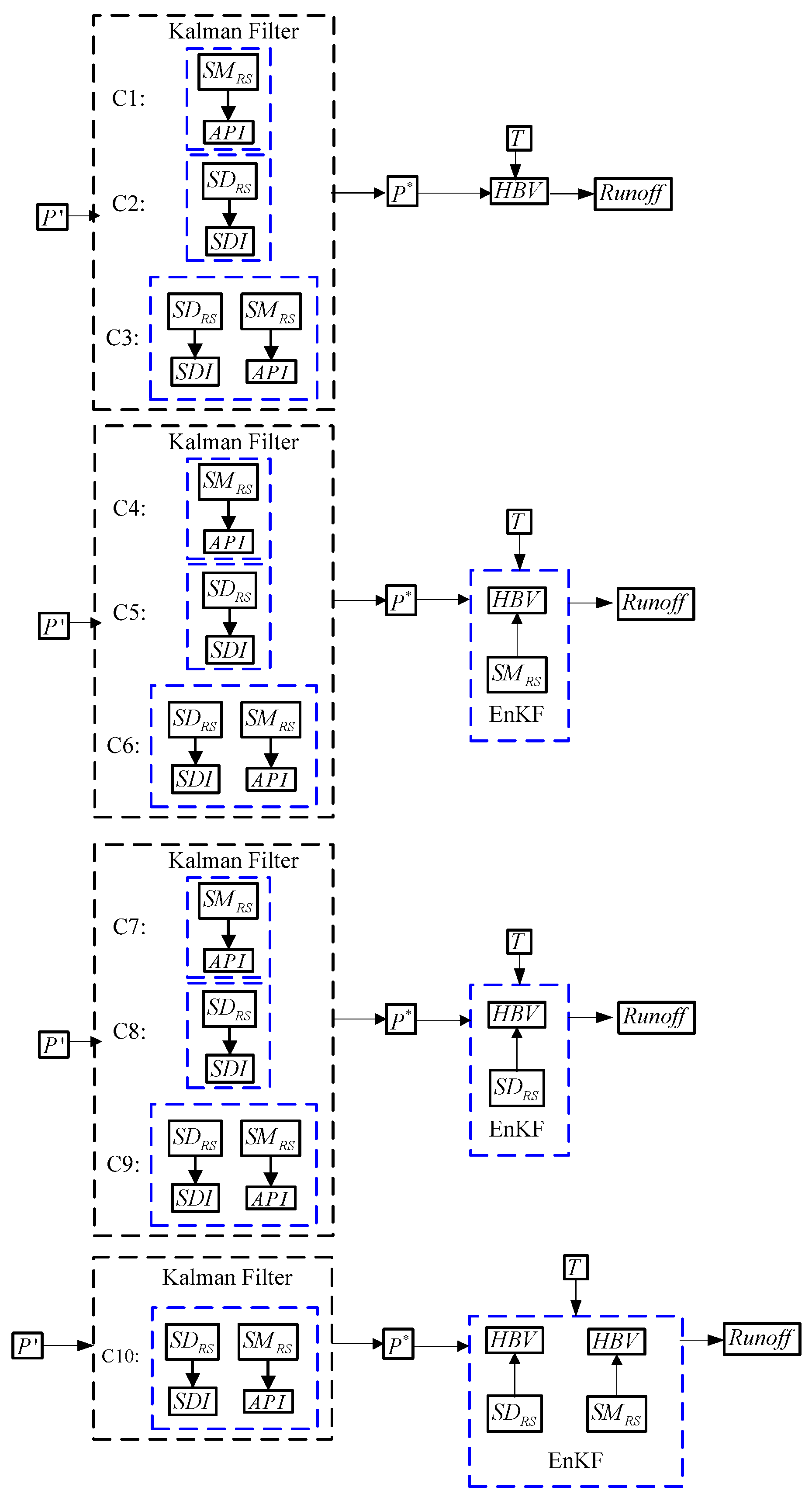
2.6. Synthetic Experiments

Our primary synthetic analysis focuses on comparing runoff results derived from the 10 separate data assimilation cases (organized into four groups) outlined in Figure 1. These groups are categorized based on the EnKF state correction strategy that each employs (i.e., no state correction, SD-based cold season correction only, SM-based warm-season correction only and combined year-around SM and SD-based correction). Each of these groups is further sub-divided based on the correction strategy applied to simultaneously correct precipitation forcing data.
The first group of cases (C1, C2 and C3) are based on the application of SMART, SDART or SMART+SDART to correct only precipitation forcing. No state correction is attempted. In particular, C1 utilizes the SMART method to correct liquid precipitation only during the warm season (May–September), and C2 utilizes the SDART method to correct solid precipitation only during the cold season (October–April). Likewise, C3 is based on the combined application of both SMART and SDART to provide year-round precipitation correction. In all cases, corrected precipitation accumulations are used to force the HBV model. Note that, as described above, cases C1, C2, and C3 do not involve the direct assimilation of SM or SD retrievals to correct HBV soil moisture or snow pack model states. Instead, these three cases attempt to improve runoff prediction only through the correction of the precipitation forcing fed into the HBV model.
The second group of cases (C4, C5 and C6) mirrors the first group of three cases in terms of the precipitation correction strategy but also adds a state correction component via the EnFK-based SM assimilation during the warm season. That is, C4 attempts SMART precipitation correction and simultaneous SM-based state correction via EnKF-based during the May to September warm season. Cases C5 and C6 are analogous (with respect to EnKF-based SM assimilation), but instead described results for cold season SDART correction and year-round SMART+SDART precipitation correction strategies, respectively. Note that none of these cases in this group assimilates SD retrievals to update HBV model states.
The third group of cases (C7, C8 and C9) illustrated in Figure 1 are analogous to the second group (C4, C5 and C6) except that EnKF assimilation is based on the cold season (October–April) assimilation of cold season SD retrievals (in place of warm season SM retrievals).
The final group comprises only a single case (C10) and represents the most complete correction strategy. That is, the cold season correction of snowfall using SDART and EnKF-based assimilation of SD combined with warm season correction of liquid precipitation using SMART and the EnKF-based assimilation of SM. As a result, it alone provides complete simultaneous state and precipitation correction throughout the seasonal cycle.
Cases 4–10 illustrate the concept of dual state/forcing correction whereby RS-based SM and SD retrievals are used to simultaneously improve both external HBV precipitation forcing and internal HBV model states [24]. If improperly applied, such dual correction can imperil the assumption of mutual independence between model forecast errors and assimilated observations which underlies the application of an EnKF. Here, such error (deleterious) cross-correlation is avoided by following the approach of Crow and Ryu [6] and Chen et al. [7] and feeding SMART and SDART-corrected precipitation into an off-line realization of the HBV which has been initialized using the EnKF analysis. Streamflow output from this realization are taken to represent final DA streamflow predictions. However, state predictions derived from these off-line HBV simulations are discarded and not recycled back into the EnKF analysis. This ensures that the EnKF analysis remains optimal. See Crow and Ryu [6] for further discussion.

2.7. Error Models for Data Assimilation Experiments

The first portion of our analysis is based on results derived from the use of synthetic data assimilation experiments. Such experiments utilize RS SM and SD predictions derived from a single integration of the HBV model as synthetic truth and derive observed SM and SD values via the introduction of synthetic additive noise to degrade such synthetic truth. In addition, daily precipitation accumulations (both solid and liquid phase) acquired from TRMM Version 3B40RTv7 (see below) are synthetically perturbed. These artificially perturbed forcing datasets are then used to force HBV model simulations—leading to random error in HBV state and streamflow predictions. Various data assimilation approaches are evaluated based on the degree to which the assimilation of (synthetically-perturbed) SM and SD observations are able to correct these random modeling errors.
In particular, perturbed rainfall is generated by multiplying actual rainfall with a mean-unity lognormal random variable:
P R S = δ P × P t r u e ,   δ P Log N ( 1 , ω p )
Likewise, air temperature is perturbed via synthetic additive error:
T o b s = T t r u e + δ T
where δ T was sampled from a mean-zero normal distribution with a variance of 4 ((°C)2). The variances in Equations (23) and (24) are assumed to be constant in time. Unless otherwise noted, ω p = 4 (-).
In synthetic experiments, assimilated RS-based SM and SD retrievals are also perturbed via the use of synthetically-generated random noise. This noise is assumed to be serially uncorrelated, mutually-independent, and sampled from a mean zero Gaussian distribution with a standard deviation equal to 5% of the total capacity of each state. Perturbations are then additively applied to individual synthetic-truth values of SM and SD (see above).
For real data DA experiments (based on the ingestion of actual RS-based SM and SD retrievals), Equations (23) and (24) are applied to generate ensemble HBV model forecasts using a variance of 4 ((°C)2) for δ T and assuming ω p = 4 (-). As in the synthetic data case, RS-based SM and SD observation error variances for real data assimilation experiments are assumed to be equal to 5% of the total capacity of each state.

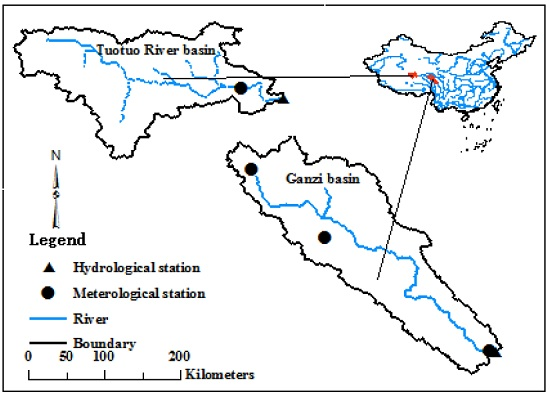
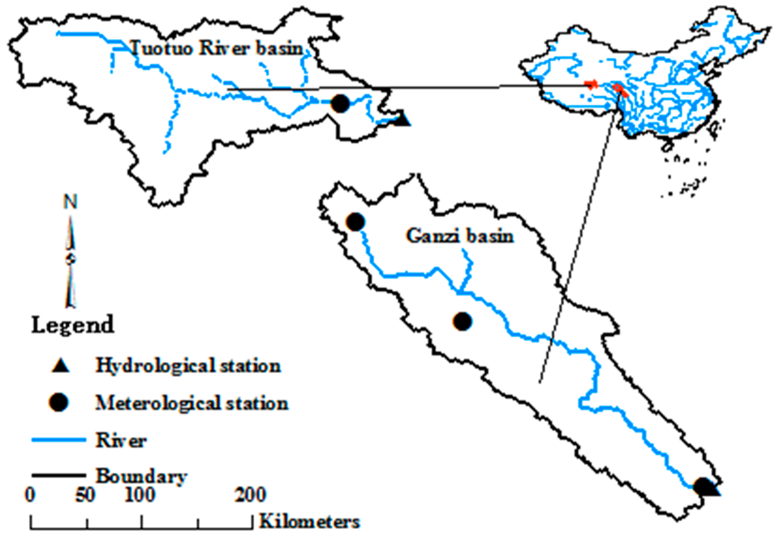
2.8. Ground Sites and Remote Sensing Data

Results are based on the application of this approach to two alpine Chinese basins: the Tuotuo River Basin at the headwaters of the Yangtze River and the Ganzi River Basin within the Himalayan plateau. The 15,924 km2 Tuotuo River Basin (Figure 2) lies at the source of the Yangtze River within the Qianggengdi mountain range of the Tibetan Plateau. The annual average precipitation within the basin is about 280 mm. During the 6-month rainy season (from May to September), the basin receives around 91% of this annual precipitation total. The annual average temperature is about −4.2 °C. The hottest month is July with an average temperature of 7.5 °C, and the coldest month is January and the month average temperature is −24.8 °C. In the streamflow observation period, the average annual discharge at the basin outlet is 26.2 m3/s with an observed daily maximum discharge of 750 m3/s. Observed precipitation and temperature data are collected from three weather ground-based stations located within the basins: the Wudaoliang (35.22° N, 93.08° E) station, the Tuotuo River (34.21° N, 92.43° E) station, and the Qumalai (34.13° N, 95.78° E) station. All station reported data during the period 1992–2011. Outlet streamflow data for the Tuotuo River Basin is available from 1992 to 1999 and then again from 2007 to 2011.
The 32,925 km2 Ganzi Basin is located in the southeastern Tibetean Plateau (Figure 2). The basin has an average elevation of around 3500 m and receives 650 mm of precipitation per year or more. Relative to the Tuotuo River Basin, the Ganzi Basin receives a much higher fraction of its annual precipitation between October and April (30% versus only 9% for the Tuotuo River Basin). In addition, because of high altitude and low temperatures, solid precipitation commonly occurs over a large fraction of the year, and summer snow fall is often seen in areas of basins above 4000 m in elevation. For example, at the 4418 m Qingshuihe weather station snowfall contributes about 40%–70% of the annual precipitation total. At the lower elevation Wenbo weather station (3900 m), snowfall still contributes 20%–40% of annual precipitation. As a result, streamflow at the Ganzi hydrological station is strongly-driven by spring melting of the snow pack.
Observed precipitation and temperature data are collected from three weather ground-based stations located in the Ganzi Basin: the Qingshuihe (33.8° N, 97.13° E) station, the Shiqu (32.97° N, 98.10° E) station, and the Ganzi (30.04° N, 101.96° E) station. All station reported data during the period 2007–2015. Outlet monthly streamflow data for the Ganzi Basin is available during the period 2007–2015. However, no daily data is available prior to 2010.
Remotely-sensed precipitation is based on TRMM (Tropical precipitation Measurement Mission) Multi-satellite Precipitation Analysis (TMPA) version 3B40RTv7 retrievals [36,37] which have been biased-corrected via the approach in Habib et al. (2014). This is a real-time microwave-only product generated without any supporting ground-based rain gauge observations. In the analysis presented below, it is applied in all instances that a precipitation time series is required (e.g., for model streamflow calibration, the generation of synthetic DA experiments, and during real data DA experiments) except for the calibration of the SMART and SDART λ factors described in Section 2.4 and Section 2.5. Due to its requirement for an independent precipitation product, this calibration is instead based on the sparse ground-based precipitation observations described above.
The ASCAT surface SM product used for this study covers the period 2009–2013 [38]. However, the vertical support of these retrievals is relatively shallow (0–5 cm) and not reflective of deeper root-zone soil moisture conditions. To obtain a deeper root zone SM product (SWI, soil water index) from the satellite-based surface observation, the semi-empirical exponential filtering approach developed by Wagner et al. [38] is adopted. For details, see Albergel et al. [10] or Wagner et al. [38].
SD data products for China were provided by the Chinese Cold and Arid Regions Science Data Center. Based on passive microwave observations obtained from the SMMR (1978–1987), SSM/I (1987–2008) and AMSR-E (2002–2012) sensors, this data provides daily coverage of SD from 24 October 1978 to 31 December 2012 at a spatial resolution of 25 km. Since all three of these sensors are mounted on different satellite platforms, there are mutual inconsistencies between them. Here, such inconsistencies are minimized via the cross-calibration of brightness temperature observations obtained from each sensor. Then, using the modified algorithm of Che et al. [39], SD retrievals within China are inverted from the cross-calibrated brightness temperatures [40]. Finally, the background data from passive microwave SD is calibrated based on ground measurements [5].

3. Results

All analysis is based on calibration of the HBV model against outlet streamflow observations acquired for both the Tuotuo River and Ganzi Basins (Section 3.1). This calibrated version of the HBV model is then utilized both as the basis for synthetic data assimilation experiments (Section 3.2) and as the assimilation model for a real data assimilation analysis (Section 3.3). Real data assimilation results are verified via actual daily streamflow observations obtained at both basin outlets.

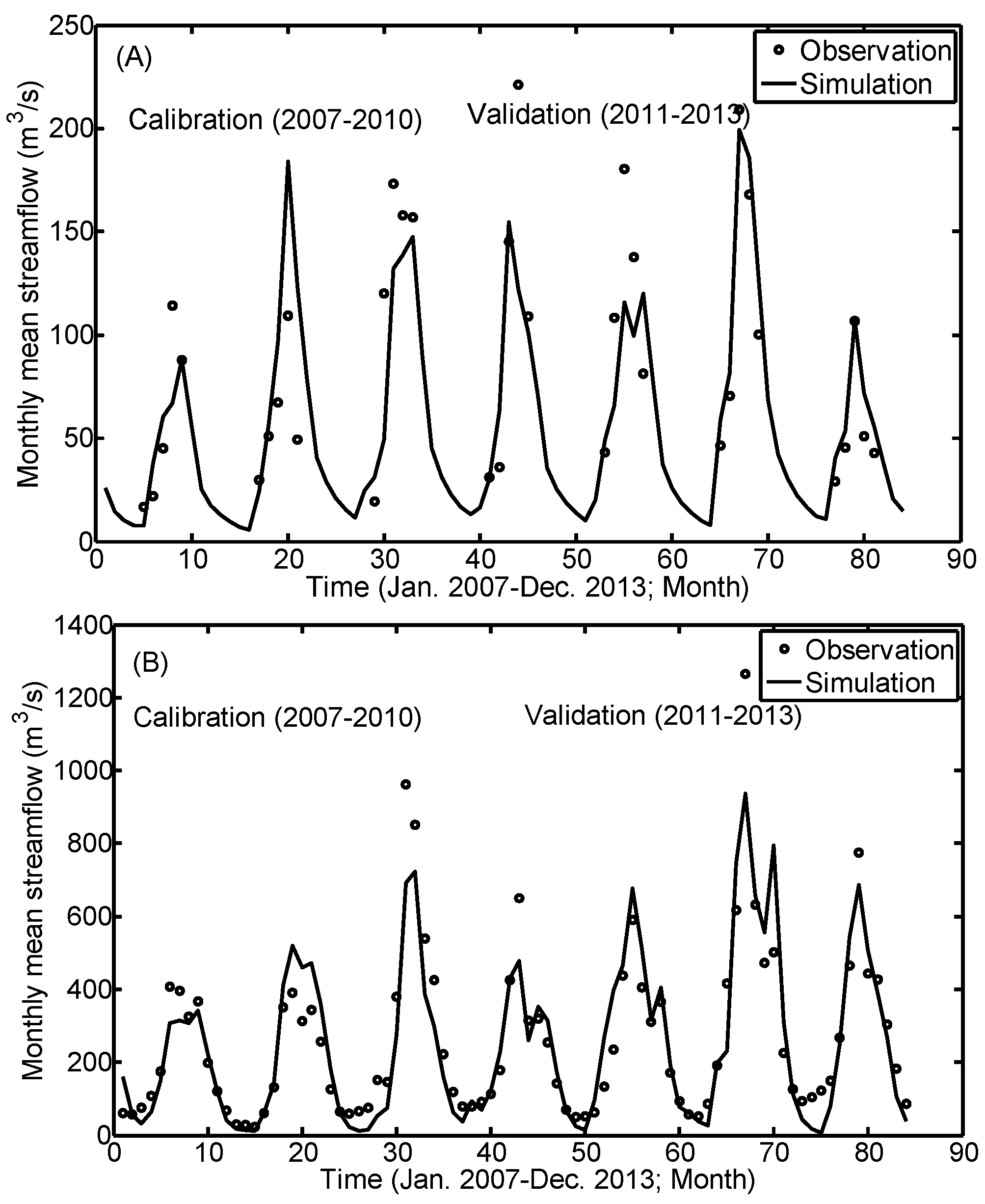
3.1. HBV Calibration and Validation

The HBV model is used to simulate daily streamflow within the Tuotuo River and Ganzi Basins between 2007 and 2013. Since the Tuotuo River hydrology station is a flood season station, observed streamflow data is only available between May and September of each year. In addition, due to restrictions on the availability of daily runoff data, calibration is based on monthly streamflow observations acquired at the Tuotuo and Ganzi hydrology stations.
Taking into account the period of the available TRMM Version 3B40RTv7 and the period of the available observed streamflow, the period 2007–2010 is reserved for calibration purposes and the period 2011–2013 for validation within both basins. In order to realistically reflect the lack of ground-based precipitation observations within most headwater basins, calibration results are based on forcing the HBV model with daily TRMM Version 3B40RTv7 data. The calibration objective function is defined using the following criteria: (1) the absolute error (AE) of the annual runoff is close to zero; (2) the Nash-Sutcliffe (NS) efficiency of monthly runoff is close to one as possible; and (3) the correlation coefficient of the observed monthly runoff (R) is close to one as possible. The objective function is defined by
f ( v ) = w 1 f 1 ( v ) +   w 2 f 2 ( v )   + w 3 f 3 ( v )
where f 1 ( v ) = AE, f 2 ( v ) = 1 − NS and f 3 ( v ) = 1 − R2 and w i = 1 / 3 ( i = 1 , 2 , 3 ). The SCE-UA optimized method is employed to minimize Equation (25) [26,41]. Final calibrated HBV model parameters are listed in Table 1 for both basins. These parameters are applied in all subsequent HBV-based DA experiments described below.
Figure 3 plots monthly streamflow predictions obtained from these calibrated HBV simulations. At the Tuotuo River hydrology station, calibration yields monthly HBV model streamflow predictions with a Nash-Sutcliffe coefficient of 0.69 (-) for the calibration period (2007–2010) and 0.62 (-) for the validation (2011–2013) period. At a daily time scale, this same set of optimized parameters yields a daily Nash-Sutcliffe coefficient of 0.49 (-) for the calibration period and 0.56 (-) for the validation period. At the Ganzi hydrology station, a Nash-Sutcliffe coefficient of HBV predicted monthly runoff of 0.89 (-) is obtained for the calibration period and 0.85 (-) for the validation period (Figure 3). No daily streamflow data is available prior to 2010 for the calculation of daily streamflow metrics within the Ganzi Basin. Post-calibration, a positive monthly bias of 25.6 m3/s is found for HBV streamflow estimates within the Tuotuo River Basin. Likewise, a positive bias of 66.4 m3/s is found within the Ganzi Basin.
It should be acknowledged that both basins are relatively large for the application of a spatially-lumped hydrology model like HBV. However, the lumped nature of the HBV model does not prevent us from obtaining reasonably good streamflow calibration results in both basins (Figure 3).

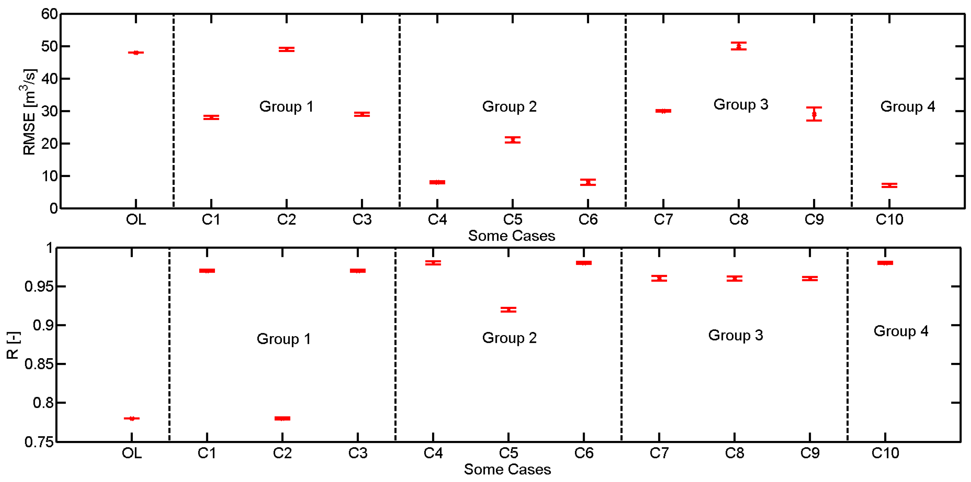
3.2. Synthetic Experiment Results

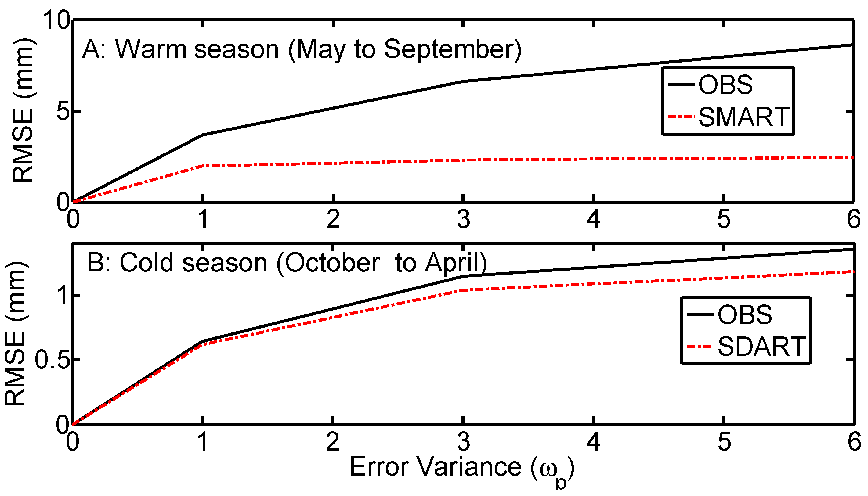
3.2.1. Impact of Precipitation Error

Figure 4 is based on a set of synthetic experiment results applied within the Tuotuo River Basin. It shows the root-means-square-error (RMSE) accuracy of corrected daily and areal average precipitation time series for all both SMART and SDAR over a range of precipitation error variances (i.e., ω p = 0,1,3,6 in Equation (23)). As described above, daily and true SM and SD data are obtained by forcing the calibrated version of HBV model using TRMM-based precipitation and observed air temperature, and the HBV-simulated SM and SD time series is perturbed using the random error models described in Section 2.7 to obtain S M R S and S D R S . These synthetically-generated observations are then applied via SMART and SDART models to correct artificially-perturbed liquid and solid precipitation accumulations, respectively.
Figure 4A shows the RMSE of the SMART-corrected precipitation and observed precipitation during the warm season (May to September) within the Tuotuo River Basin. All precipitation is represented as a summed daily accumulation. Since precipitation occurs mainly during the summer period, when it has a direct impact on soil moisture dynamics, the application of SMART is capable of substantially improving RS-based liquid precipitation estimates. Not surprisingly, absolute errors in corrected precipitation products increase as a function of ω p (Figure 4). However, the relative improvement in corrected precipitation (versus the uncorrected, original precipitation) also becomes larger as ω p increases. For example, consider the relative reduction in precipitation RMSE or R M S E o b s R M S E c o r R M S E o b s × 100 % . Based on results in Figure 4A, if ω P = 1 (-), the relative RMSE reduction percentage is 47%. If ω P = 6 (-), this percentage increases to 70%. Therefore, SMART has the greatest relative impact on cases where the background liquid precipitation is of relatively low quality.
Figure 4B shows analogous results except for the RMSE of corrected precipitation product using SDART during the cold season within the Tuotuo River Basin. Overall relative reductions in precipitation RMSE are lower for SDART in Figure 4B than for SMART in Figure 4A. Nevertheless, clear improvement is observed. For example, assuming ω P = 1 (-) the reduction rate of RMSE for SDART is 7.8% for solid precipitation. This reduction rate increases to 13.8% for ω P = 6 (-). Therefore, as in the case of liquid precipitation, increased error in measured precipitation ( ω p ) is associated with a larger fractional reduction in SDART-corrected daily snowfall accumulations.
Although correction rates for liquid precipitation are relatively high. Figure 4A,B confirm the feasibility of correcting both liquid and solid precipitation accumulations using remotely-sensed observations. Based on this assessment, the next section will examine the impact of such precipitation correction on basin outlet streamflow predictions.

3.2.2. Streamflow Correction

Figure 5 plots the RMSE and R of HBV streamflow predictions obtained from synthetic data assimilation experiments for all 10 data assimilation cases summarized in Figure 1. Because of sampling uncertainty in the Monte Carlo noise sampled for each synthetic DA experiment, all experiments are conducted using 50 independent experiments (each utilizing a unique random number sequence to generate replicates) and plotted results represent the ensemble mean and 95% confidence interval (CI) for streamflow RMSE and correlation R metrics sample across these multiple replicates. The Open Loop (OL) case plotted in Figure 5 refers to the case of running the (synthetically-perturbed) HBV model without any data assimilation. As a result, it serves as a performance datum that all subsequent data assimilation results should improve upon. As described above, the 10 data assimilation cases illustrated in Figure 1 can be categorized into four groups based on the combination of precipitation and/or state-correction strategies they each employ.
The first group of results (corresponding to cases C1, C2, and C3) are based on the application of SMART and SDART to correct precipitation forcing only. For this group, no state correction of any kind is attempted. Plotted results in Figure 5 demonstrate that case C1 (SM-based SMART correction only) and case C3 (SM-based SMART correction during the warm season and SD-based SDART correction during the cold season) yield superior streamflow results relative to case C2 (SD-based SDART correction only) and the HBV open loop datum. The relative superiority of cases based on the correction of warm season rainfall (i.e., C1 and C2) is not surprising due to relatively low levels of snowfall in the basin and the tendency for snow accumulation to impact streamflow only during a relatively brief spring snow melt season.
The second group of results (corresponding to cases C4, C5, and C6) are based on the simultaneous correction of both precipitation and HBV internal states via the EnKF assimilation of RS-based SM (see Figure 1). Note the SM state updating is applied only during warm season months since SM cannot be reliability retrieved in the presence of snowpack and/or frozen soils. Due to the added (positive) impact of SM data assimilation, results for this group are relatively superior to those seen earlier in cases C1, C2 and C3. For example, we see a 57% reduction in RMSE when moving between case C1 (based solely on warm season SM-based rainfall correction) and case C4 (warm season SM-based rainfall correction plus SM-based state correction). Similar results are seen when comparing cases C2 and C5 and cases C3 and C6. In all cases, the incorporation of SM-based data assimilation has a clear beneficial impact on streamflow RMSE and R which is in addition to the (previously-described) benefit of only correcting HBV precipitation forcing.
The third group of results (corresponding to cases C7, C8 and C9) is based on the simultaneous correction of both precipitation plus HBV internal states via the cold season EnKF assimilation of RS-based SD. Streamflow RMSE results for this group are larger than corresponding results in Group 2 (based on the SM data assimilation). This suggests that, for this particular basin, the impact of SD-based state updating, while generally positive, is smaller than that of SM.
The Group 1 and Group 3 cases are based on the same set of corrected precipitation forcing. The only difference between them (i.e., C1 vs. C7, C2 vs. C8, and C3 vs. C9) is that HBV state variables are directly corrected using SD retrievals in Group 3 while no state correction is performed for Case 1. Despite the introduction of this state correction, there is no obvious improvement in Group 3 streamflow simulations. In addition, the uncertainty (i.e., 95% confidence spread) of R and RMSE evaluation results for case C9 is larger than for case C3. This implies that a relatively small improvement may be associated with the use of SD for direct state correction and motivates the (alternative) use of SD to improve solid precipitation forcing for the HBV model.
Group 4 (containing only the single case C10) reflects the maximal possible use of all RS-based SM and SD observations to simultaneously correct both year-round forcing precipitation and year-round HBV model states (i.e., SD in the cold season and SM during the warm season). As a result, simulated streamflow results for case C10 are superior to any other case in terms of either streamflow R or RMSE.
Results in Figure 5 can be summarized as follows. Of the two retrieval types, RS-based SM observations appear more valuable when used to either improve HBV precipitation inputs (compare Cases C1 and C2 results in Figure 5) or when applied via EnKF-based state correction (compare Group 2 to Group 3 results in Figure 5). Nevertheless, the best possible results are obtained for Case C10 which incorporates both SM and SD retrievals to simultaneously correct external precipitation forcing and internal HBV model states. Plotted 95% confidence intervals in Figure 1 provide a measure of expected sampling uncertainty in plotted R and RMSE error metrics.

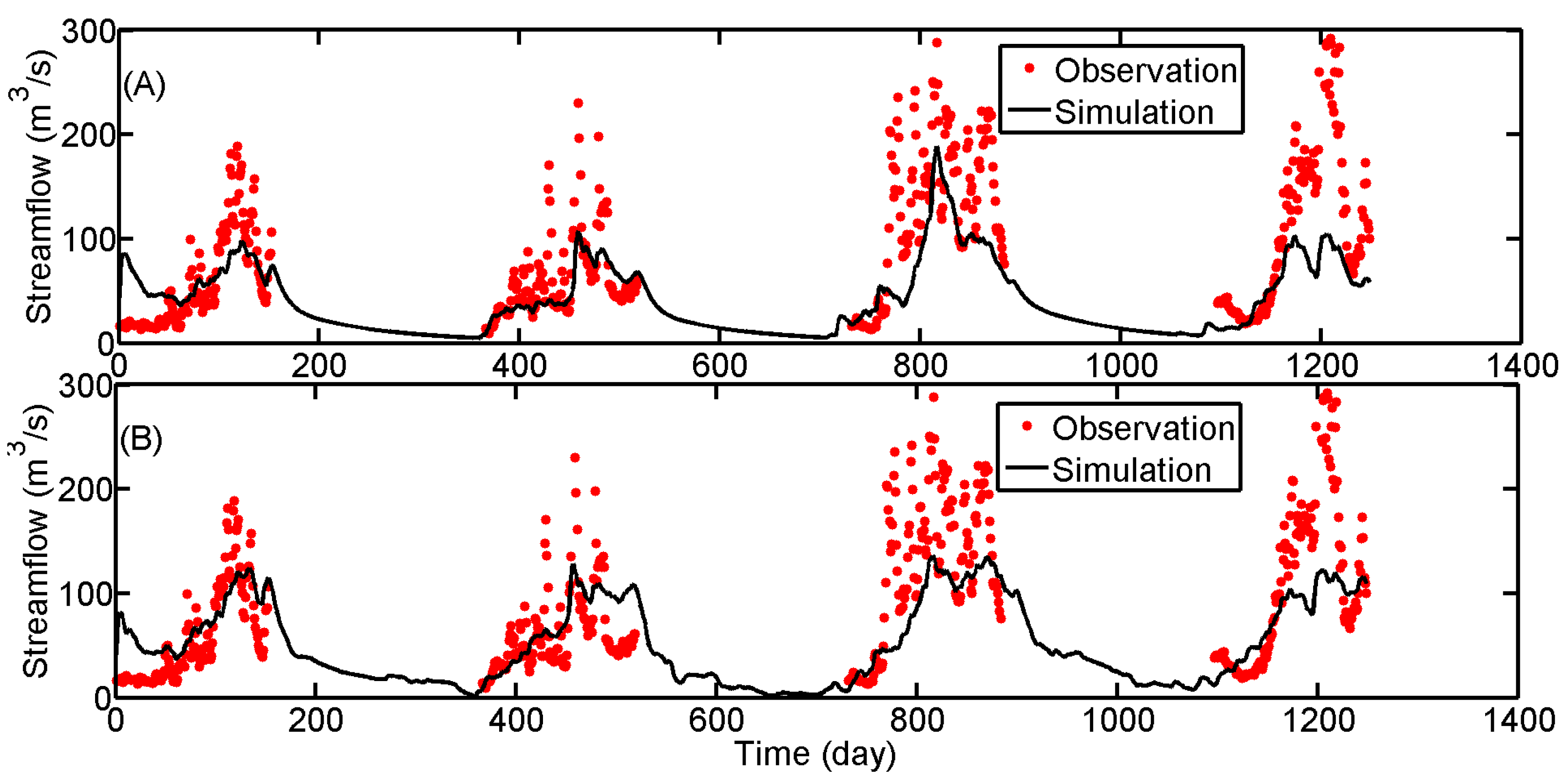
3.3. Real Data Experiment Results

In addition to the synthetic results shown above, selected DA cases are also examined within real DA assimilation experiments and verified using independent streamflow observations acquired at the outlet of both the Tuotuo River and Ganzi Basins.

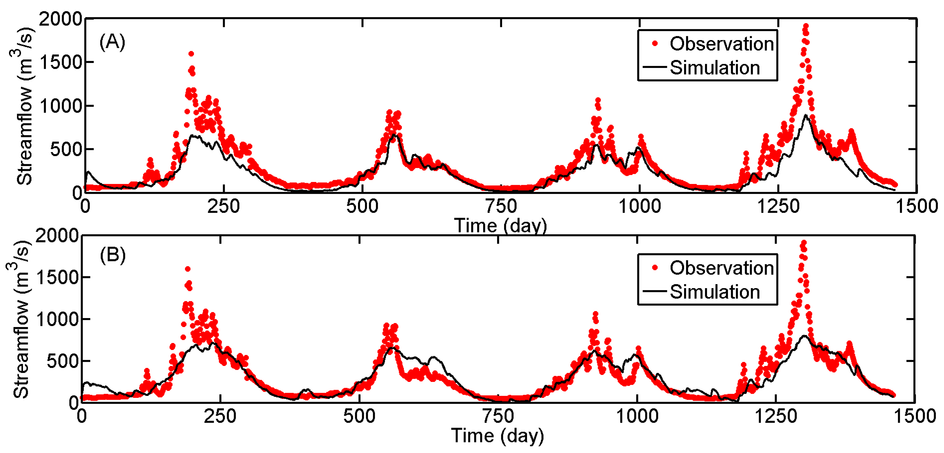
3.3.1. Tuotuo River Basin

Streamflow observations are available at the outlet of the Tuotuo River basin. However, observation conditions at the hydrological station are difficult and significant uncertainty exists when utilizing streamflow observations for model verification. In addition, streamflow observations are only available between May and September. As a result, only 612 actual days of data are available during the simulation period (2007–2011). On the other hand, because of uncertainty in RS-estimated rainfall estimates, it is necessary to use multi-source data assimilation to improve rainfall-runoff simulations.
Results shown in Figure 6 are based on a real data assimilation experiment utilizing actual RS-based SM and SD. This figure plots HBV-estimated streamflow for the Open Loop (i.e., no assimilation) HBV case and data assimilation case C10 between 1 May 2007 and 30 September 2010. As described above, case C10 is based on the maximal use of RS-based SD and SM data to simultaneous correct both HBV precipitation inputs (using SMART and SDART) and year-round HBV state variables (i.e., SD during the cold season and SM during the warm season). Earlier synthetic results (shown in Figure 5) suggest that case C10 represents the optimal approach for improving streamflow results via the simultaneous integration of RS-based SM and SD. As a result, real data results presented in Figure 6 are based only on comparisons between it and the Open Loop case.
Due to the dual correction of both HBV states and forcing precipitation data applied in case C10, simulated streamflow in case C10 deviates significantly from the HBV Open Loop baseline (which lacks any DA). In particular, case C10 DA results exhibit more low-frequency temporal dynamics than the baseline HBV Open Loop case.
Statistical fit criteria for daily streamflow predictions within the Tuotuo River Basin are summarized in Table 2. Relative to the baseline Open Loop case, the C10 data assimilation case improves the NS of predicted streamflow from 0.32 to 0.50 (-). However, other statistical measures of streamflow accuracy are only slightly improved. For example, the RMSE for case C10 is only slightly less than for the Open Loop case (55 versus 49 m3/s). Likewise, case C10 and the Open Loop exhibit the same daily correlation with respect to steamflow observations. Therefore, it should be noted that while small improvements are noted, the relative magnitude of improvement (between case C10 and the Open Loop) is considerably smaller in the real data experiments relative to earlier synthetic results summarized in Figure 5. In addition, due to the relatively short (and auto-correlated) streamflow record, these differences are not clearly significant.
For the cold season period between October and April, the streamflow of the case C10 is consistently larger than that predicted by the Open Loop case (see Figure 6A). For example, the mean of the simulated streamflow in the dry winter season is 19.15 m3/s for the Open Loop case versus 26.05 m3/s for the DA C10 case. However, due to a complete lack of validating streamflow observations during the cold season within the Tutuo River Basin, it is impossible to determine whether or not this increase actually represents an improved description of streamflow.

3.3.2. Ganzi Basin

Real data assimilation experiments were also conducted within the Ganzi Basin (see Figure 2). Relative to the Tuotuo River Basin, the Ganzi Basin has more cold season precipitation and receives a larger streamflow contribution from glacial melt water and seasonal snowpack melting. For the Ganzi Basin, Figure 7 plots: (1) observed streamflow; (2) the HBV-estimated streamflow for the Open Loop case; and (3) the analyzed streamflow for the C10 data assimilation case.
The statistical fit criteria of daily streamflow predictions within the Ganzi Basin are summarized in Table 2. The results of these comparisons are qualitatively consistent with earlier results in the Tuotuo River Basin. That is, while small NS and RMSE improvements are noted in C10 data assimilation case (relative to the Open Loop baseline), they are smaller than improvements realized in our synthetic DA experiments (Figure 5).
During the whole simulation period, simulated streamflow for both the C10 and Open Loop cases is biased flow relative to observations within the Ganzi Basin. In particular, the Open Loop case has about −28% relative bias. This bias is reduced somewhat (to −6.56%) for data assimilation of case C10. However, such a reduction should be viewed with skepticism since neither the state nor the forcing correction components of case C10 are designed to reduce long-term bias. It is quite possible that the apparent reduction of bias is due to spurious bias canceling via the introduction of bias terms in the EnKF process associated with nonlinearities in the HBV model [42].
Note that DA results in Figure 6B and Figure 7B both show instances of over correction where DA converts a minor overestimation of streamflow into more significant underestimation (see e.g., results around day 1000 in Figure 7B). At short time scales, such artifacts are common in data assimilation systems and likely associated with seasonal biases in assimilated RS-based SM or SD retrievals. However, over the long term, optimal DA procedures should minimize the overall RMSE in streamflow estimates.

3.3.3. Flood Peak Values

In addition to long-term RMSE, R, NS, streamflow results should be evaluated based on their ability to capture peak streamflow values. The flood peak is impacted by the magnitude and distribution of precipitation, antecedent SM and SD conditions in the basin and data assimilation strategies et al. Although, NS of C10 is larger than Open Loop, NS is low in both basins. The simulated flood peaks for cases C10 all significantly underestimate the observed peak in both watersheds (see Figure 6B and Figure 7B). This tendency is clear for the summer of 2009 in the Tuotuo River Basin and for the 2009 and 2012 summers in the Ganzi Basin. This reduction in flow peak magnitude appears to be due to the tendency of SMART to under predict extreme rain fall intensities and the EnKF-based state correction to under predict saturated soil moisture conditions. Such an inability to accurately characterize extremes is a known problem with data assimilation referred to as “conditional bias” whereby DA tends to underestimate maximum value and over-estimate minimums of state value because the spatial scale of the RS data is often coarse. Conditional bias has been previously observed in attempts to correct RS-based precipitation using soil moisture time series [43]. Nevertheless, it should be acknowledged that none of the data assimilation approaches presented here appears particularly well suited for the estimation of peak streamflow volumes.
Adding streamflow into the observation vector (along with RS-based SM and SD) is an obvious extension of this work which could conceivably improve the characterization of streamflow peaks. However, it should be stressed that, in many headwater basins, daily streamflow observations are not operationally available. In such basins, remotely-sensed soil moisture and soil depth measurements represent the sum total of daily observations which are available for assimilation within an operational hydrological forecasting system. Therefore, significant practical barriers exist for the direct assimilation of streamflow.

4. Conclusions

Using RS-based SM and AD data to improve streamflow simulation is a critical challenge in cold region hydrology. A key aspect of this challenge is the tendency for error to originate concurrently in both internal model state dynamics (used to describe antecedent soil moisture conditions) and external model forcing (most notably precipitation). Typical data assimilation approaches apply RS-based SM and SD retrievals to correct only the first source of error (via internal state correction) and do not address the impact of random forcing errors on runoff and streamflow predictions.
This paper describes a new version of SMART model-referred to as the Snow Depth Analysis Rain Tool or SDART-that utilizes RS SM data to also correct solid precipitation accumulation during the cold season. Corrected precipitation (in both the liquid and solid phase) obtained from SMART and SDART is then employed to force the HBV hydrological model. Simultaneously, an EnKF is applied to assimilate RS-based SM retrievals into the HBV model during snow-free conditions and RS-based SD estimates when snow is present on the ground. That is, a dual assimilation system is developed to simultaneously update HBV forcing and state variables within both the warm and cold seasons.
Ten separate synthetic DA cases within the Tuotuo River Basin are considered. These synthetic experiments demonstrate that the application of the SMART or SDART methods leads to a clear improvement in the quality of daily accumulations of both liquid and solid phase daily precipitation. In particular, the best streamflow results are acquired via the dual use of both SMART/SDART to correct year-round precipitation and the simultaneous assimilation of both RS SD and SM retrievals to correct internal HBV snow and soil moisture states (i.e., DA case C10).
These synthetic DA experimental results were augmented via real DA results based on the use of TRMM version 3B40RTv7 retrievals as RS precipitation data source, ASCAT surface SM results and a multi-sensor (SMMR, SMM/I and AMSR-E) SD analysis provided by the Chinese Cold and Arid Regions Science Data center. For the real data experiments, results from two watersheds (the Tuotuo River and Ganzi Basin—see Figure 1) are examined. Based on long-term RMSE, NS and R streamflow results obtained in these real data experiments, the simultaneous correction of both external precipitation forcing and internal model states (i.e., DA case C10) represents the most efficient approach for improving streamflow results via the use of RS-based SM and SD retrievals (see Table 2). Such an approach can be applied to both liquid precipitation during the warm season (using SMART) or solid precipitation during the cold season (using SDART).
However, it should be noted that all DA results exhibit evidence of condition bias—particularly a clear inability to accurately capture streamflow peaks. In addition, due to the marked auto-correlation of the streamflow time series used for validation, sampling uncertainties for verification metrics listed in Table 1 are likely to be large. As a result, the relatively modest improvements in RMSE, R and NS associated with DA (relative to the baseline Open Loop case) currently lack statistical significance. Additional study is required to better assess and/or correct these tendencies.
As discussed above, the study basins utilized here are relatively large for the application of the spatially-lumped HBV model. Therefore, the extension of the approach to a spatially-distributed modeling approach represents an obvious path for future research. However, it should be stressed that, due to the relatively coarse spatial resolution (~25 km–50 km) of the SM and SD products assimilated here, these approaches can be applied to enhance only coarse-scale precipitation patterns. Therefore, except for applications involving very large basins (>100,000 km2), the marginal value of distributed hydrologic modeling may be relatively low for the data assimilation approaches described here.
Nevertheless, using the SMART and SDART algorithms, RS SM and RS SD retrievals can be used to operationally-correct liquid and solid phase precipitation accumulation estimates obtained from satellite-based RS. By appropriately applying these corrected accumulations within a hydrological data assimilation system, RS SM and RD can be maximally leveraged to improve streamflow monitoring and predications in un-gauged headwater basins with significant cold season precipitation. Future work will focus on the geographic expansion of our proposed system and improved DA performance during high-flow periods.

Acknowledgments

This research was supported by National Basic Research Program of China (2013CBA01806), NNSF (41371049; 41571015; 41323001; 51190091), Fund of State Key Laboratory of Hydrology-Water Resources and Hydraulic Engineering (20145027312) and the open fund of State Key Laboratory of Desert and Oasis Ecology, Xinjiang Institute of Ecology and Geography.

Author Contributions

Haishen Lü and Wade T. Crow conceived and designed the paper and experiments; Yonghua Zhu and Fen Ouyang analyzed the data; Jianbin Su contributed the figures; all authors collaborated to write the paper.

Conflicts of Interest

The authors declare no conflict of interest.

Abbreviations

The following abbreviations are used in this manuscript:
SMSoil moisture
SDSnow depth
SMOSSoil Moisture and Ocean Salinity
SMAPSoil Moisture Active/Passive
ASCATAdvanced Scatterometer
METOPMeteorological Operational
RSRemotely-sensed
DAData assimilation
SMARTSoil Moisture Analysis Rainfall Tool
SDARTSnow Depth Analysis Rainfall Tool
HBVHydrologiska Byrans Vattenbalansavdelning
EnKFEnsemble Kalman filter
SCEShuffled Complex Evolution
SWISoil water index
OLOpen Loop

References

  1. Alvarez-Garreton, C.; Ryu, D.; Western, A.W.; Su, C.H.; Crow, W.T.; Robertson, D.E.; Leahy, C. Improving operational flood ensemble prediction by the assimilation of satellite soil moisture: Comparison between lumped and semi-distributed schemes. Hydrol. Earth Syst. Sci. 2015, 19, 1659–1676. [Google Scholar] [CrossRef]
  2. Aubert, D.; Loumagne, C.; Oudin, L. Sequential assimilation of soil moisture and streamflow data in a conceptual rainfall-runoff model. J. Hydrol. 2003, 280, 145–161. [Google Scholar] [CrossRef]
  3. Brocca, L.; Melone, F.; Moramarco, T.; Wagner, W.; Naeimi, V.; Bartalis, Z.; Hasenauer, S. Improving runoff prediction through the assimilation of the ascat soil moisture product. Hydrol. Earth Syst. Sci. 2010, 14, 1881–1893. [Google Scholar] [CrossRef]
  4. Thirel, G.; Salamon, P.; Burek, P.; Kalas, M. Assimilation of MODIS snow cover area data in a distributed hydrological model. Hydrol. Earth Syst. Sci. Discuss. 2011, 8, 1329–1364. [Google Scholar] [CrossRef]
  5. Kumar, S.V.; Peters-Lidard, C.D.; Mocko, D.; Reichle, R.; Liu, Y.; Arsenault, K.R.; Xia, Y.; Ek, M.; Riggs, G.; Livneh, B.; et al. Assimilation of remotely sensed soil moisture and snow depth retrievals for drought estimation. J. Hydrometeorol. 2014, 6, 2446–2469. [Google Scholar] [CrossRef]
  6. Crow, W.; Ryu, D. A new data assimilation approach for improving runoff prediction using remotely-sensed soil moisture retrievals. Hydrol. Earth Syst. Sci. 2009, 13, 1–16. [Google Scholar] [CrossRef]
  7. Chen, F.; Crow, W.T.; Starks, P.J.; Moriasi, D.N. Improving hydrologic predictions of a catchment model via assimilation of surface soil moisture. Adv. Water Res. 2011, 34, 526–536. [Google Scholar] [CrossRef]
  8. Lü, H.; Hou, T.; Horton, R.; Zhu, Y.; Chen, X.; Jia, Y.; Wang, W.; Fu, X. The streamflow estimation using the xinanjiang rainfall runoff model and dual state-parameter estimation method. J. Hydrol. 2013, 480, 102–114. [Google Scholar] [CrossRef]
  9. Kerr, Y.H.; Waldteufel, P.; Wigneron, J.P.; Martinuzzi, J.; Font, J. Soil moisture retrieval from space: The soil moisture and ocean salinity (smos) mission. IEEE Trans. Geosci. Remote. Sens. 2001, 39, 1729–1735. [Google Scholar] [CrossRef]
  10. Albergel, C.; Rüdiger, C.; Carrer, D.; Calvet, J.C.; Fritz, N.; Naeimi, V.; Bartalis, Z.; Hasenauer, S. An evaluation of ascat surface soil moisture products with in-situ observations in southwestern france. Hydrol. Earth Syst. Sci. 2009, 13, 115–124. [Google Scholar] [CrossRef]
  11. Bartalis, Z.; Wagner, W.; Naeimi, V.; Hasenauer, S.; Scipal, K.; Bonekamp, H.; Figa, J.; Anderson, C. Initial soil moisture retrievals from the metop-a advanced scatterometer (ascat). Geophys. Res. Lett. 2007, 34, L20401. [Google Scholar] [CrossRef]
  12. Goodrich, D.C.; Schmugge, T.J.; Jackson, T.J.; Unkrich, C.L.; Keefer, T.O.; Parry, R.; Bach, L.B.; Amer, S.A. Runoff simulation sensitivity to remotely sensed initial soil water content. Water Resour. Res. 1994, 30, 1393–1405. [Google Scholar] [CrossRef]
  13. Weissling, B.P.; Xie, H.; Murray, K.E. A multitemporal remote sensing approach to parsimonious streamflow modeling in a southcentral texas watershed, USA. Hydrol. Earth Syst. Sci. Discuss. 2007, 4, 1–33. [Google Scholar] [CrossRef]
  14. Parajka, J.; Naemi, V.; Bloschl, G.; Wagner, W.; Merz, R.; Scipal, L. Assimilating scatterometer soil moisture data into conceptual hydrologic models at coarse scales. Hydrol. Earth Syst. Sci. 2006, 10, 353–368. [Google Scholar] [CrossRef]
  15. Pauwels, V.R.N.; Hoeben, R.; Verhoest, N.E.C.; De Troch, F.P.; Troch, P.A. Improvement of toplats-based discharge predictions through assimilation of ers-based remotely sensed soil moisture values. Hydrol. Process. 2002, 16, 995–1013. [Google Scholar] [CrossRef]
  16. Crow, W.T.; Bindlish, R.; Jackson, T.J. The added value of spaceborne passive microwave soil moisture retrievals for forecasting rainfall-runoff partitioning. Geophys. Res. Lett. 2005, 32, L18401. [Google Scholar] [CrossRef]
  17. Brocca, L.; Moramarco, T.; Melone, F.; Wagner, W. A new method for rainfall estimation through soil moisture observations. Geophys. Res. Lett. 2013, 40, 853–858. [Google Scholar] [CrossRef]
  18. Wood, E.F.; Sivapalan, M.; Beven, K. Similarity and scale in catchment storm response. Rev. Geophys. 1990, 28, 1–18. [Google Scholar] [CrossRef]
  19. Crow, W.; van Den Berg, M.; Huffman, G.; Pellarin, T. Correcting rainfall using satellite-based surface soil moisture retrievals: The soil moisture analysis rainfall tool (smart). Water Resour. Res. 2011, 47, 2924–2930. [Google Scholar] [CrossRef]
  20. Pellarin, T.; Ali, A.; Chopin, F.; Jobard, I.; Bergs, J.-C. Using spaceborne surface soil moisture to constrain satellite precipitation estimates over west africa. Geophys. Res. Lett. 2008, 35, L02813. [Google Scholar] [CrossRef]
  21. Chen, F.; Crow, W.T.; Holmes, T.R.H. Improving long-term, retrospective precipitation datasets using satellite-based surface soil moisture retrievals and the soil moisture analysis rainfall tool. J. Appl. Remote Sens. 2012, 6, 063604. [Google Scholar] [CrossRef]
  22. Lindströ, G.; Johansson, B.; Persson, M.; Gardelin, M.; Bergströ, S. Development and test of the distributed hbv-96 hydrological model. J. Hydrol. 1997, 201, 272–288. [Google Scholar] [CrossRef]
  23. Aghakouchak, A.; Habib, E. Application of a conceptual hydrologic model in teaching hydrologic processes. Int. J. Eng. Educ. 2010, 26, 1–11. [Google Scholar]
  24. Lu, H.; Crow, W.T.; Zhu, Y.; Yu, Z.; Sun, J. The impact of assumed error variances on surface soil moisture and snow depth hydrologic data assimilation. IEEE J. Sel. Top. Appl. Earth Obs. Remote. Sens. 2015, 8, 5116–5129. [Google Scholar]
  25. Duan, Q.; Sorooshian, S.; Gupta, V.K. Optimal use of the sce-ua global optimization method for calibrating watershed models. J. Hydrol. 1994, 158, 265–284. [Google Scholar] [CrossRef]
  26. Moradkhani, H.; Sorooshian, S.; Gupta, H.V.; Houser, P.R. Dual state-parameter estimation of hydrological models using ensemble kalman filter. Adv. Water Resour. 2005, 28, 135–147. [Google Scholar] [CrossRef]
  27. Vrugt, J.A.; Gupta, H.V. Real-time data assimilation for operational ensemble streamflow forecasting. J. Hydrometeorol. 2006, 7, 548–564. [Google Scholar] [CrossRef]
  28. Crow, W.T.; Huffman, G.J.; Bindlish, R.; Jackson, T.J. Improving satellite-based rainfall accumulation estimates using spaceborne surface soil moisture retrievals. J. Hydrometeorol. 2009, 10, 199–212. [Google Scholar] [CrossRef]
  29. Kienzle, S.W. A new temperature based method to separate rain and snow. Hydrol. Process. 2008, 22, 5067–5085. [Google Scholar] [CrossRef]
  30. Bergström, S. Development and Application of a Conceptual Runoff Model for Scandinavian Catchments; SMHI Report: Norrköping, Sweden, 1976; p. 134. [Google Scholar]
  31. Pipes, A.; Quick, M.C. Ubc Watershed Model Users Guide; Department of Civil Engineering; University of British Columbia: Vancouver, BC, Canada, 1977. [Google Scholar]
  32. Leavesley, G.H.; Lichty, R.W.; Troutman, B.M.; Saindon, L.G. Precipitation-Runoff Modeling System: User’s Manual; Water Resources Investigations Report 83–4238; Us Geological Survey: Denver, CO, USA, 1983.
  33. Wen, L.J.; Nagabhatla, N.; Lü, S.H.; Wang, S.Y. Impact of rain snow threshold temperature on snow depth simulation in land surface and regional atmospheric model. Adv. Atmos. Sci. 2013, 30, 1449–1460. [Google Scholar] [CrossRef]
  34. Cherry, J.E.; Tremblay, L.B.; Der.Stephen, J.; Stieglitz, M. Reconstructing solid precipitation from snow depth measurements and a land surface model. Water Resour. Res. 2005, 41, W09401. [Google Scholar] [CrossRef]
  35. Zhang, Y.; Liu, S.; Ding, Y. Observed degree-day factors and their spatial variation on glaciers in western china. Ann. Glaciol. 2006, 43, 301–306. [Google Scholar] [CrossRef]
  36. Huffman, G.J.; Adler, R.F.; Bolvin, D.T.; Nelkin, E.J. The trmm multi-satellite precipitation analysis (tmpa). In Satellite rainfall Applications for Surface Hydrology; Springer: Berlin, Germany, 2010; pp. 3–22. [Google Scholar]
  37. Yong, B.; Hong, Y.; Ren, L.L.; Gourley, J.J.; Huffman, G.J.; Chen, X.; Wang, W.; Khan, S.I. Assessment of evolving trmm-based multisatellite real-time precipitation estimation methods and their impacts on hydrologic prediction in a high latitude basin. J. Geophys. Res. Atmos. 2012, 117, D9. [Google Scholar] [CrossRef]
  38. Wagner, W.; Lemoine, G.; Rott, H. A method for estimating soil moisture from ers scatterometer and soil data. Remote. Sens. Environ. 1999, 70, 191–207. [Google Scholar] [CrossRef]
  39. Che, T.; Xin, L.; Jin, R.; Armstrong, R.; Zhang, T. Snow depth derived from passive microwave remote-sensing data in china. Ann. Glaciol. 2008, 49, 145–154. [Google Scholar] [CrossRef]
  40. Che, T.; Dai, L. China Snow Depth Time Series Data Sets (1978–2012); Cold and Arid Regions Science Data Center at Lanzhou: Lanzhou, China, 2011. [Google Scholar]
  41. Parajka, J.; Merz, R.; Blöschl, G. Uncertainty and multiple objective calibration in regional water balance modelling: Case study in 320 Austrian catchments. Hydrol. Process. 2007, 21, 435–446. [Google Scholar] [CrossRef]
  42. Chen, F.; Crow, W.T.; Ryu, D. Dual forcing and state correction via soil moisture assimilation for improved rainfall-runoff modeling. J. Hydrometeorol. 2014, 15, 1832–1848. [Google Scholar] [CrossRef]
  43. Ryu, D.; Crow, W.T.; Zhan, X.; Jackson, T.J. Correcting unintended perturbation biases in hydrologic data assimilation using ensemble kalman filter. J. Hydrometeorol. 2009, 10, 734–750. [Google Scholar] [CrossRef]
Figure 1. The flowchart for data assimilation cases C1–C10.
Remotesensing 08 00503 g001
Figure 2. Location of the Tuotuo River Basin and Ganzi Basin in Western China.
Remotesensing 08 00503 g002
Figure 3. HBV model simulated and observed average monthly streamflow within designated calibration (2007–2010) and validation (2011–2013) periods at the outlet of the (A) Tuotuo River Basin and the (B) Ganzi Basin.
Remotesensing 08 00503 g003
Figure 4. The RMSE of corrected (A) SMART- and (B) SDART-corrected precipitation for various levels of (synthetically-introduced) precipitation error.
Remotesensing 08 00503 g004
Figure 5. Daily streamflow flow RMSE and correlation (R) results for synthetic data assimilation experiments based on the application of the Open Loop (OL) HBV model (with no DA) and the 10 DA cases (C1 to C10) outlined in Section 2.6 and Figure 1.
Remotesensing 08 00503 g005
Figure 6. Daily observed streamflow at the outlet of the Tuotuo River Basins for both: (A) Open Loop HBV simulated results obtained without data assimilation and (B) case C10 data assimilation results between 1 May 2007 and 30 September 2010.
Remotesensing 08 00503 g006
Figure 7. Daily observed streamflow at the outlet of the Ganzi Basin for both: (A) Open Loop HBV simulated results obtained without data assimilation and (B) case C10 data assimilation results between 1 January 2010 and 21 December 2013.
Remotesensing 08 00503 g007
Table 1. Parameters, state variables, inputs and outputs (with ranges) for the HBV model.
Parameters, Variables, Input and OutputPhysical MeaningRangeTuotuo River BasinGanzi River Basin
ParametersDD (L·θ−1·T−1)Degree-day factor3–74.96.89
β (–)Model shape coefficient1–71.331.05
FC (L )Maximum soil storage capacity100–200200199
C (θ−1)Evapatranspiration parameter0.01–0.070.030.01
PWP (L)Soil permanent wilting point90–18094.1690.02
K0 (T−1)Recession coefficients0.05–0.20.080.2
K1 (T−1)Recession coefficients0.02–0.10.050.05
K2 (T−1)Recession coefficients0.02–0.050.010.03
L (L)Threshold water level2–1005044
Kp (T−1)Percolation storage coefficient0.01–0.050.040.04
State variablesSD (L)Snow depth
SM (L)Soil moisture
SU (L)Upper reservoir water level
SL (L)Lower reservoir water level
InputP (L)Precipitation
T (θ)Temperature
OutputQs (L3T−1)Total simulated runoff
Ea (L)Actual evapotranspiration
Table 2. Statistical criteria of daily streamflow simulation in two watersheds for two cases.
WatershedCriteriaOpen LoopC10
Tuotuo RiverRMSE (m3/s)5549
NS (-)0.320.50
R (-)0.720.72
Ganzi RiverRMSE (m3/s)169159
NS (-)0.650.70
R (-)0.890.90

