Joint Model and Observation Cues for Single-Image Shadow Detection

Abstract

Shadows, which are cast by clouds, trees, and buildings, degrade the accuracy of many tasks in remote sensing, such as image classification, change detection, object recognition, etc. In this paper, we address the problem of shadow detection for complex scenes. Unlike traditional methods which only use pixel information, our method joins model and observation cues. Firstly, we improve the bright channel prior (BCP) to model and extract the occlusion map in an image. Then, we combine the model-based result with observation cues (i.e., pixel values, luminance, and chromaticity properties) to refine the shadow mask. Our method is suitable for both natural images and satellite images. We evaluate the proposed approach from both qualitative and quantitative aspects on four datasets. The results demonstrate the power of our method. It shows that the proposed method can achieve almost 85% F-measure accuracy both on natural images and remote sensing images, which is much better than the compared state-of-the-art methods.

1. Introduction

Shadows, which are cast by elevated objects, such as buildings, trees, and clouds, are ever-present phenomena in remote sensing and computer vision. Shadow is a double-edged sword for image interpretation, depending on whether the shadows are modeled or ignored. Additional semantic and geometric cues provided by shadows help us to localize objects. However, shadows can also degrade the accuracy of several tasks (e.g., image classification [1], change detection [2], object recognition [3], image segmentation [4], etc.) due to spurious boundaries and confusion between shading and reflectivity. For these reasons, shadow detection has become a crucial pre­processing stage of scene interpretation.

Many shadow detection techniques have been proposed in the last decade. One type is based on interaction, called semiautomatic methods [5]. Interaction-based methods can achieve good performance results where user-supplied information should be provided. For example, in Wu and Tang [6], a quadmap that defines the candidate shadow and non-shadow regions is required in their Bayesian framework. Wu et al. [7] formulated shadow detection as a matting problem, and users were asked to give several strokes to specify shadows and non-shadows. Despite these methods being accurate, their requirements will dramatically reduce efficiency. Furthermore, incorporating them into a fully automatic workflow is difficult.

Compared with semi-automatic methods, fully-automatic methods have drawn much more attention in recent years. These methods can be divided into two types: single-image approaches and multi-image approaches [5]. Tsai [8] observed that shadow regions have the property of lower luminance, but higher hue values, and a ratio map can be constructed for the detection problem. Zhang et al. [9] proposed an object-based method. The authors used a thresholding technique to extract suspected shadow objects and rule out dark objects based on spectral properties and shape information. 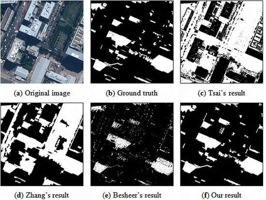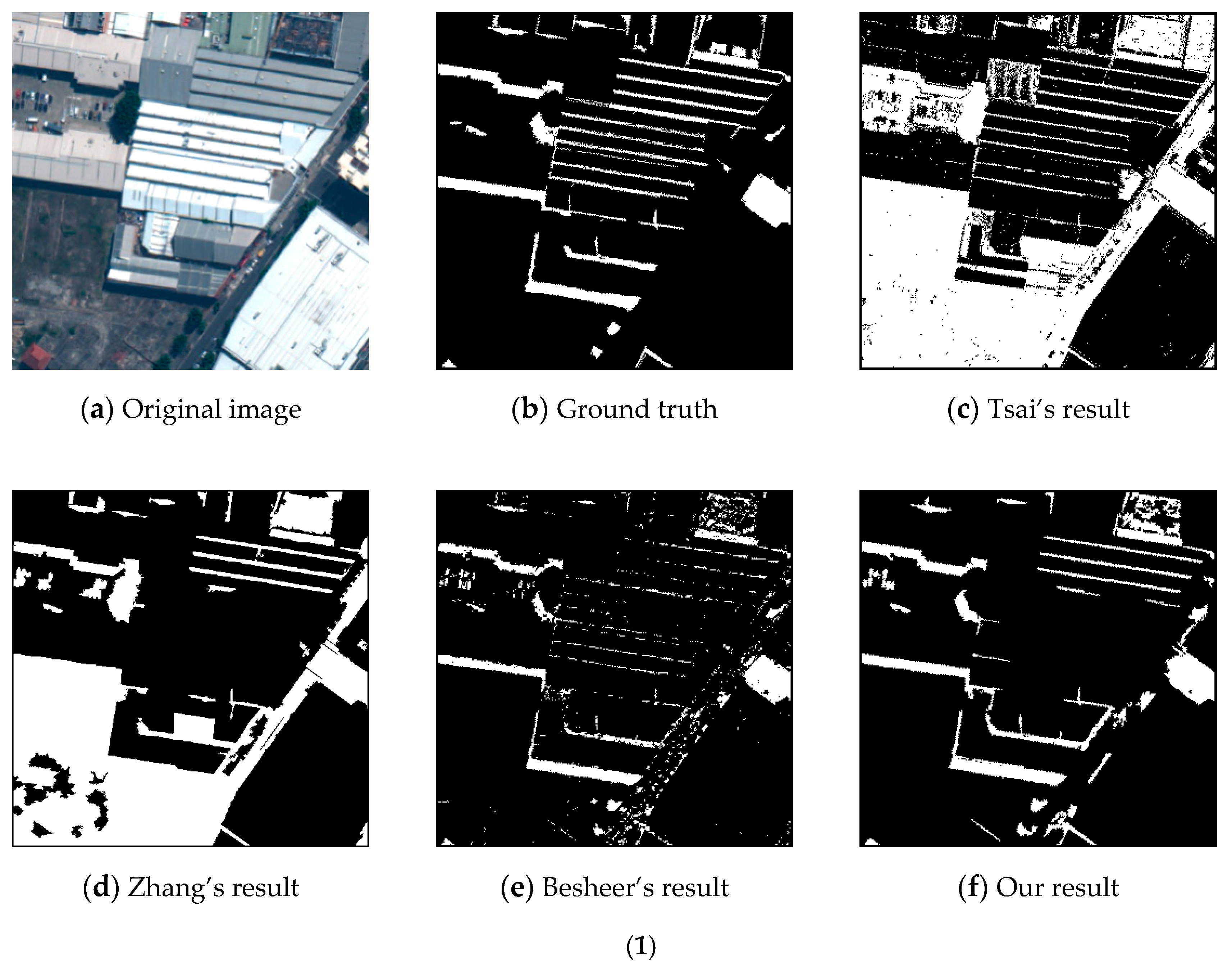Besheer and Abdelhafiz [10] improved the original C1C2C3 invariant color model using near-infrared (NIR) channel information. The authors used bimodal histogram splitting to provide the threshold of binary segmentation. Their method is only suitable for images with a NIR channel. In [11], an algorithm that uses both spatial and spectral features was proposed. Similar to the method by Zhang et al., this method is also based on the thresholding technique and object segmentation. Risson presented a shadow detection method in his thesis using a photometric analysis approach to recover lighting conditions of color images [12]. Panagopoulos et al. [13] presented a method based on bright channel cues. The authors used the bright channel to provide an adequate approximation to the illumination component. Then, they adapted a Markov random field (MRF) to refine the bright channel. Boundary information is also a powerful cue to distinguish shadows from non-shadows, such as in [14,15,16]. These methods use only pixel or edge information, which may become limitations in more complicated scenes. To improve robustness, several model-based methods have been studied. Finlayson et al. [17] obtained illumination-invariant images by projecting an image’s log chromaticities based on the Planckian illumination model. Panagopoulos et al. [18] presented a higher-order Markov random field (MRF) model to recover the illumination map. An impressive performance can be achieved with high-quality images and calibrated sensors, but a poor performance is achieved for typical web-quality photographs [19]. Tian et al. [20,21] proposed a trichromatic attenuation model (TAM) and combined it with pixel intensity to classify shadow pixels. Data-driven approaches, which is another popular technique, learn a shadow detection model from a training set. Guo et al. [22] used a region-based approach. In their work, a relational graph of paired regions is adopted for the problem. Zhu et al. [23] learned statistical information. i.e., intensity, gradient and texture, to classify regions in monochromatic images. More recently, Khan et al. [24,25] proposed an extremely impressive shadow detection framework based on multiple convolutional deep neural networks. This model learns features at the superpixel level and along dominant boundaries; then, smooth shadow masks are detected via a conditional random field model.

To transform the ill-posed problem of recovering an intrinsic image from a single photograph to a well-posed one, other studies have been performed in which multiple images (or additional information) are considered. For example, Weiss [26] recovered an intrinsic reflectance image based on an image sequence of the same scene with varying illumination conditions. Tolt et al. [27] analyzed the line-of-sight on a DSM and estimated the position of the sun to assist illumination component extraction. Drew et al. [28] proposed a method to estimate the illumination map by combining flash/no-flash image pairs. These methods can easily obtain an accurate shadow map. However, their application is extremely restricted because most of the scenes do not satisfy their requirements, e.g., the flash/non-flash method may fail in an outdoor environment.

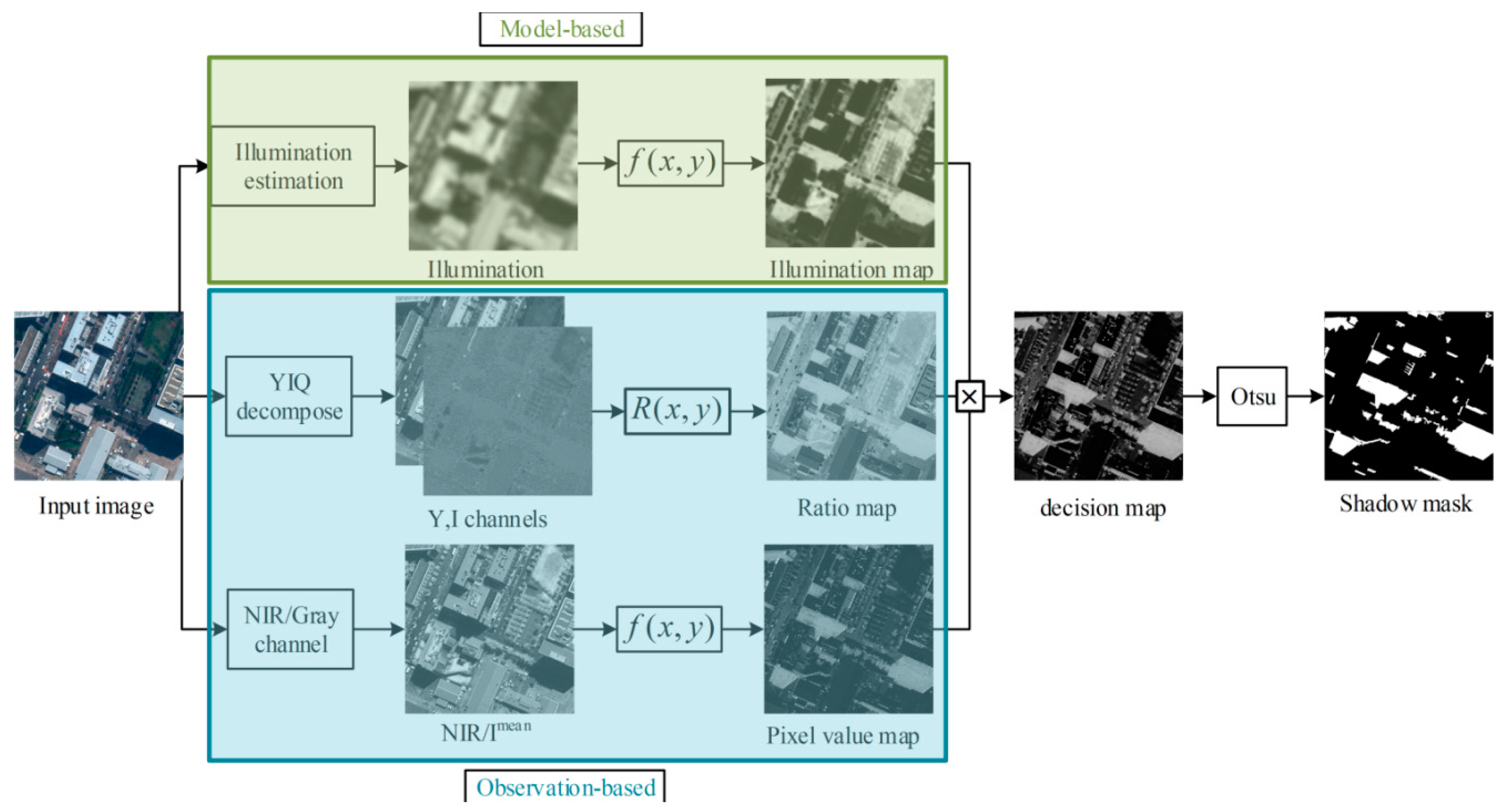
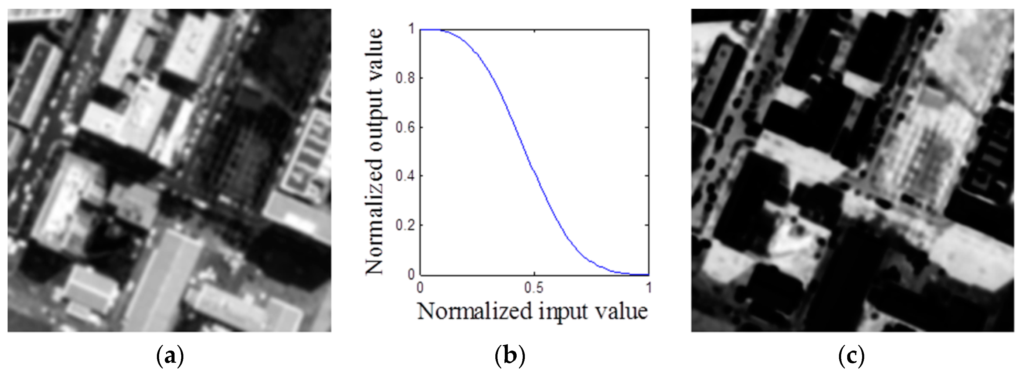
In this paper, we address the shadow detection problem for more complex scenes based only on a single image. Different from the method of Panagopoulos et al. [13], whose bright channel cue gives an approximation of the illumination component, our method gives a bright channel prior for the radiance component. We join the model and observation cues to improve the detection accuracy. Firstly, an approximate occlusion map is estimated using a simple prior, called the bright channel prior (BCP). Then, a ratio map and a pixel value map are produced based on the properties of the shadows. Afterwards, the final decision map is generated by fusing these three feature maps to segment out shadows. We evaluate our method from both qualitative and quantitative aspects on two datasets. The results demonstrate that our method is effective for the shadow detection task.

The contributions of our work are summarized as follows:

(1)

We derive a new formulation of the original BCP and adapt the radiance-based BCP for shadow detection task; and

(2)

We combine the model cue with several observation cues (i.e., pixel values, luminance and chromaticity properties) to improve detection accuracy. Our method is suitable for both natural images and remote sensing images. We also use NIR channel information (if a NIR channel is available) to distinguish dark objects from shadows. Despite the simplicity of the proposed method, a high detection accuracy can be achieved and does not require any post-processing stages.

2. Methods

2.1. Properties of a Shadow

Shadows are created wherever the light source is occluded, which means that illumination in shadow regions is lower than that in non-shadow regions. If we can exactly estimate the illumi­nation component of the scene image, the problem is solved. However, recovering illumination from only a single image is an ill-posed problem. Several hypotheses or priors are typically introduced for simplicity at the cost of losing accuracy. To improve the robustness of model-based approaches, several observation cues can be introduced, i.e., pixel values, luminance and chromaticity properties. Thus, shadows are characterized by the following properties:

(1)

Lower illumination component in the illumination-reflectance model;

(2)

Lower luminance but higher hue values in photometric invariant color models, such as YIQ [11]; and

(3)

Lower pixel intensity, except dark objects in the RGB color model.

Based on these properties, we propose a framework to join the model and observation cues to exactly detect shadows. Figure 1 shows the schematic diagram of the proposed method, in which the green box and the blue box represent the model-based and observation-based shadow detection parts, respectively. The input of our approach is a single color image with a NIR channel, if possible. After performing model-based and observation-based shadow detection, three shadow feature maps are produced. Then, a final decision map is generated by simply fusing these feature maps, and Otsu’s method is adapted to segment out the shadow mask, which is the output of the proposed framework.

2.2. Model-Based Shadow Detection

2.2.1. Illumination-Reflectance Model

In image processing and computer vision, the illumination-reflectance model [29] is broadly adopted to describe the formation of an image. This model defines that the image of a scene I can be divided into two components, i.e., illumination L and reflectance R. Working from the model, we simply improve the illumination term to make its physical interpretation for shadow detection clearer. In detail, the illumination component is decomposed into a uniform illumination A, which is also called global atmospheric light, and an occlusion map F, whose dark values represent the possible occlusion areas, such that the final model can be formulated as:

$$\mathit{I}(x,y)=A\mathit{F}(x,y)\mathit{R}(x,y)$$

(1)

Our goal is to recover $A$ and $\mathit{F}$ from $\mathit{I}$. Unfortunately, this is an underdetermined system of equations, and hypotheses or priors should be introduced in advance.

2.2.2. Bright Channel Prior

The dark channel prior [30] is a famous statistic-based prior for image dehazing. Motivated by this, Wang et al. [31] proposed a similar prior for image exposure enhancement, called the bright channel prior, which is based on the following observation: in most well-exposed image patches, there are several pixels with an extremely high intensity in at least one color channel. In other words, the maximum intensity in such a color patch should have an extremely high value, which can be defined as:

$$J^{bright}(x,y)=\underset{c\in \{r,g,b)}{\max }(\underset{(x^{\prime },y^{\prime })\in \mathsf{\Omega }(x,y)}{\max }({\mathit{J}}^c(x^{\prime },y^{\prime }))\to (200~255)$$

(2)

where ${\mathit{J}}^c$ is a color channel of the well-exposed image $\mathit{J}$ and $\mathsf{\Omega }(x,y)$ represents a small local patch centered at pixel $(x,y)$.

Our goal is to detect shadows, whose detection model is different from the exposure model. Directly introducing their prior for our task is difficult; hence, we present a new modified prior. We can infer from the original bright channel prior that, in most of the image patches, at least one channel has an extremely high reflectance at certain pixels. This is the definition of our new bright channel prior. We assume that the extremely high reflectance is close to 1. Hence, it can be formulated as:

$$R^{bright}(x,y)=\underset{c\in \{r,g,b)}{\max }(\underset{(x^{\prime },y^{\prime })\in \mathsf{\Omega }(x,y)}{\max }(R^c(x^{\prime },y^{\prime }))\to 1$$

(3)

2.2.3. Illumination Map Estimation

Here, the global atmospheric light A is automatically estimated using a method similar to the one introduced in He’s de-hazing study [30]. In detail, the dark channel I^dark of scene image I is firstly computed:

$${\mathit{I}}^{dark}(x,y)=\underset{c\in \{r,g,b)}{\min }({\mathit{I}}^c(x,y))$$

(4)

Then, the pixels in the dark channel ${\mathit{I}}^{dark}$ are ranked, and the top 0.1% brightest pixels are chosen. Afterwards, the average intensity of these pixels in the corresponding input image $\mathit{I}$ is accepted as the global atmospheric light.

We denote the reflectance of the patch as $\overline{R}(x,y)$. In each small local patch, applying the max operation on the image formation model Equation (2), we obtain the following:

$$\underset{(x^{\prime },y^{\prime })\in \mathsf{\Omega }(x,y)}{\max }(I^c(x^{\prime },y^{\prime }))=A\underset{(x^{\prime },y^{\prime })\in \mathsf{\Omega }(x,y)}{\max }(F(x,y)\cdot {\overline{R}}^c(x^{\prime },y^{\prime }))$$

(5)

Notice that the max operation is performed on three color channels independently. Within a very small region, we assume that the shadows are continuous; thus, the values in the occlusion map of this region are essentially a constant value. We use ${\overline{F}}_{\mathsf{\Omega }(x,y)}$ to represent the constant occlusion value of local patch $\mathsf{\Omega }(x,y)$, and Equation (5) can be reformulated as:

$$\underset{(x^{\prime },y^{\prime })\in \mathsf{\Omega }(x,y)}{\max }(I^c(x^{\prime },y^{\prime }))\approx A{\overline{F}}_{\mathsf{\Omega }(x,y)}\cdot \underset{(x^{\prime },y^{\prime })\in \mathsf{\Omega }(x,y)}{\max }({\overline{R}}^c(x^{\prime },y^{\prime }))$$

(6)

Then, the maximum value among these color channels can be found:

$$\underset{c\in (r,g,b)}{\max }(\underset{(x^{\prime },y^{\prime })\in \mathsf{\Omega }(x,y)}{\max }(I^c(x^{\prime },y^{\prime })))\approx A{\overline{F}}_{\mathsf{\Omega }(x,y)}\cdot \underset{c\in (r,g,b)}{\max }(\underset{(x^{\prime },y^{\prime })\in \mathsf{\Omega }(x,y)}{\max }({\overline{R}}^c(x^{\prime },y^{\prime })))$$

(7)

According to our aforementioned new bright channel prior, the maximum reflectance in the local patch tends to be one, and we have:

$${\overline{R}}^{bright}(x,y)=\underset{c\in \{r,g,b)}{\max }(\underset{(x^{\prime },y^{\prime })\in \mathsf{\Omega }(x,y)}{\max }({\overline{R}}^c(x^{\prime },y^{\prime }))\approx 1$$

(8)

Combining Equations (7) and (8), the approximate occlusion value ${\overline{F}}_{\mathsf{\Omega }(x,y)}$ can be obtained:

$${\overline{F}}_{\mathsf{\Omega }(x,y)}\approx \frac{\underset{c\in (r,g,b)}{\max }(\underset{(x^{\prime },y^{\prime })\in \mathsf{\Omega }(x,y)}{\max }(I^c(x^{\prime },y^{\prime })))}{A}$$

(9)

This occlusion map contains serious block effects and is not that accurate due to the assumptions. We observe that our occlusion map exhibits similar properties with the transmission map in the dehazing methods. Motivated by this, we apply a refinement stage on $\overline{\mathit{F}}$, where either soft matting [32] or a guided filter [33] can be adapted (in this paper, we chose guided filter); then, an accurate occlusion map $\mathit{F}$ is produced:

$$\mathit{F}=g\otimes \overline{\mathit{F}}$$

(10)

where $g$ is the guided filter, and $\otimes$ represents $g$ adapting onto $\overline{\mathit{F}}$.

Once the occlusion map is obtained, the shadows can be detected by extracting the dark values in the map. To enlarge the difference between the shadows and the non-shadows and reduce the number of uncertain pixels, a non-linear mapping function is applied:

$${\mathit{S}}_{molel}=f(\mathit{F}),f(x)=e^{-\mathsf{\alpha }{x}^{\mathsf{\beta }}}$$

(11)

where ${\mathit{S}}_{molel}$ is a feature map of illumination, $\mathsf{\alpha }$ is a slope-like coefficient and $\mathsf{\beta }$ influences the range of this sigmoid function.

The non-linear mapping function $f$ has two functions: first, it inverts the dark and bright parts in the occlusion map $\mathit{F}$, similar to a tone mapping function, which ensures that shadows have high values, to be consistent with the ratio image that will be introduced in the next stage. Second, this function is able to enlarge the difference between shadow regions and non-shadow regions, which makes the shadows more distinct. As shown in Figure 2, the values of the original shadow map (Figure 2a) are reversed in Figure 2c when the non-linear mapping function $f$ (Figure 2b) is applied. Furthermore, in Figure 2c, we can see that shadows become more distinct to segment out.

2.3. Observation-Based Shadow Detection

Observation is another powerful cue for shadow detection. In this section, we extract shadow feature maps based on the two aforementioned properties. The first map created is based on the YIQ color model, and the other map is just based on the intensity of the NIR or RGB channels of the scene image. Details are as follows.

2.3.1. Ratio Map Estimation

In color images, color tone is represented by three elements—luminance, hue, and saturation—which are powerful descriptors in several special cases of image processing. For example, histogram equalization performed in an RGB color model would change the chromaticity of an image and destroy its color balance. However, in photometric invariant color models, the luminance and chromaticity are separated, and the color balance can be preserved by only applying histogram equalization in luminance. Thus, photometric-invariant color models are more suitable for tasks that must separate the luminance from chromaticity. As discussed in the above, for the second property, the hue and luminance of an image should be separated.

The YIQ color model was chosen, which is used by the National Television Standards Commission (NTSC) color TV system. In this model, Y stands for the luminance channel, and I and Q stand for the chromaticity channels, which represent hue and saturation, respectively [34].

After extracting the hue and luminance channel, the ratio map ${\mathit{S}}_{ratio}$ can be obtained by simply performing the spectral ratioing technique [11]:

$${\mathit{S}}_{ratio}=({\mathit{I}}^i+1)/({\mathit{I}}^y+1)$$

(12)

where ${\mathit{I}}^y$ and ${\mathit{I}}^i$ are the Y and I channels of image $\mathit{I}$, respectively.

Since shadows have the property of lower luminance but higher hue values, the higher ${\mathit{S}}_{ratio}$ values are possible shadow candidates.

2.3.2. Pixel Value Map Estimation

There is no doubt that the pixel intensity in a shadow region is lower than that of a non-shadow region, unless the pixel of a non-shadow region is in the dark object. This means that shadow detection based on the pixel intensity of RGB channels contains both shadows and dark objects. In fact, for satellite images, the near-infrared channel is available. The NIR channel has an extremely important property, that dark objects in the visible spectrum generally have a much larger pixel intensity in NIR [5]. For example, the intensity of trees is relatively small (dark) in an RGB color image but becomes extremely large (bright) in the NIR channel, as shown in the red box of Figure 3. Based on this point, we use the NIR channel instead of the visible spectrum to detect shadows when the NIR channel is available.

The NIR channel is more powerful than the RGB channels for shadow detection, in which shadows are distinct from dark objects. Such a property could solve the very problem that limits the most current algorithms. However, certain images do not provide the NIR channel, which would make this method useless. To increase the universality of the proposed framework, a tradeoff between accuracy and practicality is made. We use the mean channel ${\mathit{I}}^{mean}$ of the R, G, and B channels, instead of the NIR channel, when it is unavailable.

$${\mathit{I}}^{mean}=\frac{{\mathit{I}}^r+{\mathit{I}}^g+{\mathit{I}}^b}{3}$$

(13)

Only performing segmentation of the NIR channel is inaccurate because the optimal threshold is difficult to choose. To enlarge the difference between shadows and non-shadows, a non-linear mapping function $f$ is also applied:

$${\mathit{S}}_{pix}=f({\mathit{I}}^{nir}),f(x)=e^{-\mathsf{\alpha }{x}^{\mathsf{\beta }}}$$

(14)

where ${\mathit{I}}^{nir}$ is the NIR channel (if unavailable, use ${\mathit{I}}^{mean}$ instead), and ${\mathit{S}}_{pix}$ is a pixel value shadow candidate map.

2.4. Fusion and Segmentation

So far, we have obtained three shadow feature maps: the illumination map, the ratio map, and the pixel value map. Each feature map has its own limitations because either priors or observations cannot be satisfied by the total pixels in the image. We observe that all of these three maps, which have a range of [0, 1], have the same property, i.e., shadows have large values. To improve accuracy, a simple fusion stage that only multiplies these three maps is performed:

$${\mathit{S}}_d={\mathit{S}}_{molel}\cdot {\mathit{S}}_{ratio}\cdot {\mathit{S}}_{pix}$$

(15)

where ${\mathit{S}}_d$ is the final decision map. This fusion stage acts as a function that preserves large values (shadows) while decreases the unreliable values (i.e., the pixels that are large in certain maps but are small in other maps is called noise).

To segment the decision map into a binary shadow mask, the optimal threshold can be specified by the user. Though this could achieve the best results, its application is quite restricted due to requiring user inputs. Instead, we adopt Ostu’s method [35] to find the optimal threshold ${\mathsf{\theta }}_{opt}$. The binary shadow mask ${\mathit{S}}_{mask}$ is then produced by:

$${\mathit{S}}_{mask}(x,y)=\{\begin{array}{cc}1& \text{if\hspace{0.17em}}{S}_d(x,y)>{\mathsf{\theta }}_{opt}\\ 0& \text{otherwise}\end{array}$$

(16)

3. Results and Discussion

We evaluate the proposed framework in several aspects. First, we compare the three shadow feature maps with the final fused decision map to demonstrate the effectiveness of our jointed algorithm. Then, we qualitatively and quantitatively compare our method with several state-of-the-art shadow detection approaches. Finally, computation time is evaluated. In the following, we will detail the configuration of our experiments, including parameter setting, dataset information, algorithms for comparison, and quality assessment.

3.1. Settings

Parameter Setting: There are a few parameters required by the non-linear mapping function f and the guided filter in our approach. These parameters are fixed in all of the following experiments. Their values are set as follows: α = 7, β = 3, the patch size in the bright channel prior is 10 × 10 pixels, and the guided filter range is r_g = 10.

Dataset Information: Four datasets are used to evaluate our proposed shadow detection method. The first dataset is provided by Rufenacht [5], which consists of 57 indoor and outdoor color images (does not include indoor flash images); the second dataset is from Guo [22], which consists of 108 natural images; and the third dataset is the UCF shadow dataset [23], which contains 355 images. These images were captured by an ordinary digital camera without a near-infrared channel, and their image scenes are relatively simple. The binary ground truth is also provided.

Since there is no standard dataset of more complex scenes for such a task, a new satellite image dataset was created by us. This dataset consists of 25 images, which are all cropped from different satellite images with a near-infrared channel, i.e., Quickbird, Worldview 2, and Worldview 3 [36]. The image size is 500 × 500 pixels. To quantitatively evaluate our algorithm, the ground truth for the 25 images was produced manually. Note that for these satellite images, it can sometimes be difficult to identify whether a pixel is a shadow or not, even for a human, because the scenes are extremely complex, and shadows are confounded by many other unknown objects.

Algorithms for Comparison: We chose five state-of-the-art single image shadow detection algorithms for comparison, including Tsai’s method [8], Tian’s method [21], Guo’s method [22], Zhang’s method [9], and Besheer’s method [10]. Note that the comparison with Zhang’s and Besheer’s methods was only performed on the satellite image dataset. For fairness, the original implementation of Tian’s and Guo’s methods were obtained from the authors’ websites. Tsai’s, Zhang’s, and Besheer’s methods were implemented according to their papers in MATLAB because the original sources were not published. For Zhang’s method, we used the ERS [37] algorithm to segment an image into objects. All parameters were set using the authors’ suggestion.

Quality Assessment: Three standard evaluation metrics widely adapted in shadow detection task, i.e., recall, precision, and F-measure, are reported in this paper. The F-measure combines both recall and precision metrics into a single one that reflects the overall performance. Their definitions are as follows:

$$\begin{array}{c}Recall=\frac{TP}{TP+FN}\times 100\%\\ Precision=\frac{TP}{TP+FP}\times 100\%\\ F-measure=\frac{Recall*Precision}{Recall+Precision}\times 100\%\end{array}\}$$

(17)

in which $TP$, $FP$, and $FN$ are true positive, false positive, and false negative, respectively. True positive is the number of shadow pixels correctly identified; false negative is the number of shadow pixels wrongly identified; and false positive is the number of non-shadow pixels identified as shadow pixels. The values of the three metrics are all between [0%, 100%], where higher values in percentage indicate better results.

3.2. Validation

To validate our bright channel prior, observation cues as well as the joint framework. Shadows are detected based on the obtained illumination map ${\mathit{S}}_{molel}$, ratio map ${\mathit{S}}_{ratio}$, pixel value map ${\mathit{S}}_{pix}$, and fused decision map ${\mathit{S}}_d$ on the aforementioned Rufenacht’s and our satellite datasets. The results are shown in

Table 1. Shadow detection accuracy of different feature maps on the Rufenacht’s dataset.

Methods	Recall/%	Precision/%	F-measure/%
${\mathit{S}}_{molel}$	79.60	92.84	85.71
${\mathit{S}}_{ratio}$	99.10	75.21	85.52
${\mathit{S}}_{pix}$	97.93	76.67	86.00
${\mathit{S}}_d$	89.72	89.70	89.71

and

Table 2. Shadow detection accuracy of different feature maps on our satellite image dataset.

Methods	Recall/%	Precision/%	F-measure/%
${\mathit{S}}_{molel}$	79.74	57.40	66.75
${\mathit{S}}_{ratio}$	99.42	30.10	46.21
${\mathit{S}}_{pix}$	96.34	45.48	61.80
${\mathit{S}}_d$	85.52	87.06	86.28

.

As can be seen, our bright channel prior is a good prior for shadow detection, which achieves an overall accuracy (F-measure) of 85.71% and 66.75% for the simple (Rufenacht’s dataset) and complex (satellite dataset) image scenes, respectively. Its average accuracy of the two datasets is 76.23%, which outperforms the other two observation cues, whose accuracies are 65.87% and 73.9%. The results show that observation cues have better recall accuracy, but worse precision accuracy, compared with our bright channel prior. In other words, bright channel prior and observation cues are complementary. Thus, an effective fusion strategy will significantly improve the detection performance.

Our joint framework achieved the best results on both datasets. It has both a high recall accuracy and high precision accuracy, thus, yielding a high F-measure accuracy. It at least achieved 3.71% and 19.53% growth rates of F-measure compared with illumination map, ratio map, and pixel value map on simple scenes and complex ones, respectively. From these tables, we can infer that: (1) our joint framework is more robust than methods based on non-joint feature maps. The accuracy of non-joint maps significantly decreases when the scenes become complex; and (2) the near-infrared channel is more suitable for shadow detection than the ${\mathit{I}}^{mean}$ channel because our approach achieved a better accuracy on complex scenes (satellite image dataset uses the NIR channel) than that of the simple ones (ordinary image dataset that did not have a NIR channel, so the ${\mathit{I}}^{mean}$ channel was used instead).

3.3. Comparison

We evaluate the proposed approach both qualitatively and quantitatively. Figure 4, Figure 5, Figure 6 and Figure 7 show several visual results of the Rufenacht’s dataset, Guo’s dataset, UCF shadow dataset, and our satellite image dataset.

Table 3. Shadow detection results on Rufenacht’s dataset.

Methods	Recall/%	Precision/%	F-measure/%
Tsai [11]	96.90	76.44	85.46
Tian [19]	98.37	78.84	87.53
Guo [20]	19.53	71.77	30.70
Ours	89.72	89.70	89.71

,

Table 4. Shadow detection results on Guo’s dataset.

Methods	Recall/%	Precision/%	F-measure/%
Tsai [11]	86.07	66.04	74.74
Tian [19]	44.27	79.33	56.83
Guo [20]	68.07	77.74	72.58
Ours	87.51	76.83	81.82

,

Table 5. Shadow detection results on UCF shadow dataset.

Methods	Recall/%	Precision/%	F-measure/%
Tsai [11]	85.48	67.22	75.26
Tian [19]	89.87	68.19	77.54
Guo [20]	48.16	54.35	51.07
Ours	86.34	78.67	82.33

and

Table 6. Shadow detection results on our satellite dataset.

Methods	Recall/%	Precision/%	F-measure/%
Tsai [11]	95.11	33.57	49.62
Zhang [9]	90.24	56.62	69.59
Besheer [10]	58.29	82.04	68.16
Ours	85.52	87.06	86.28

present the quantitative evaluation of these four datasets.

As shown in Figure 4, Figure 5 and Figure 6, our method provides extremely impressive shadow masks. The differences between our detection results and the ground truth masks are the smallest among all compared methods. From Image 3 of Figure 4 and Image 1 of Figure 5, we can observe that all of the methods can achieve extremely good detection results when the shadows are simple and distinct from non-shadows. However, when the shadow scenes are complex, the performances of Tsai’s method, Tian’s method, and Guo’s method dramatically drop, as shown in Image 2 of Figure 4 and Image 1 of Figure 6. The segmentation-based methods have an inherent drawback, e.g., the method by Guo et al., where the detection accuracy depends on the segmentation result. If segmentation fails, the shadow mask will be incorrectly produced, as illustrated in Image 2 of Figure 4, Image 2 of Figure 5, and Image 2 of Figure 6, where the shadows are almost completely missed. Guo’s method is also based on learning, in which the features and training set play extremely important roles. The training set of Guo et al. may be too simple for this dataset because it can perform better on image scenes with simpler shadows (such as Image 3 of Figure 4 and Image 1 of Figure 5), but performs worse on others with more complex shadows.

For more complex urban scenes (as shown in Figure 7), the performance of Tsai’s method significantly decreased, whereas the performance of our method remained extremely good. The reason for this is that Tsai’s method tends to confuse shadows with dark objects, as illustrated in the figure, where streets, grass, trees, and several buildings were all identified as shadows. Zhang’s method could also not rule out dark objects, particularly dark ground, dark roads, and dark trees. In their method, the spectral differences between the blue band and the green band were used to rule out vegetation. However, it is difficult to choose the threshold, and the spectral properties may not be satisfied by different sensors. In addition, the shape information is not effective for ruling out dark roads and ground. In contrast, our method uses both illumination and NIR channel information, which can better distinguish shadows from dark objects. Besheer’s method missed many shadow pixels because their method is pixel-based, in which noise from pixels will decrease the detection accuracy.

Table 3, Table 4, Table 5 and Table 6 present the quantitative results, which clearly demonstrate the effect of our joint method. As can be seen, our method resulted in a higher F-measure accuracy on all four datasets compared with that of the state-of-the-art methods. It almost achieves 4.25%, 2.18%, and 59.01% growth rates of overall accuracy (F-measure) compared with Tsai’s, Tian’s, and Guo’s methods on Rufenacht’s dataset; 7.08%, 24.99%, and 9.24% growth rates on Guo’s dataset; and 7.07%, 4.79%, and 31.26% growth rates on the UCF shadow dataset, respectively. Compared with Tsai’s, Zhang’s, and Besheer’s methods, our method achieves 36.66%, 16.69%, and 18.12% growth rates on our satellite dataset. An analysis of these results in the tables shows that Tsai’s methods resulted in extremely impressive completeness accuracy (tended to be 1), but demonstrated poor results in correctness accuracy. Considering their definitions, we can infer that the $FN$, which is the number of shadow pixels wrongly identified, tends to be 0, and the $FP$, which is the number of non-shadow pixels wrongly identified, tends to be large. This is to say, Tsai’s methods could exactly identify shadow pixels but could not identify non-shadow pixels. Tian’s method and Guo’s method are sensitive to image scenes. For example, Tian’s method achieved good results on Rufenacht’s dataset, and the UCF shadow dataset but had poor results on Guo’s dataset; Guo’s method achieved good results on Guo’s dataset, but had poor results on the Rufenacht’s dataset and the UCF shadow dataset. Zhang’s method could not rule out dark trees and roads; thus, their precision is low. In contrast, Besheer’s method demonstrated good precision accuracy, but poor recall accuracy. Their method can be improved by extending the pixel-based method to an object-based one. In addition, Besheer’s method is not suitable for natural images due to the usage of the NIR channel.

From Table 6, we can see that Tsai’s method, Zhang’s method, and Besheer‘s method all achieved poor results on our satellite dataset, which can be explained by two reasons. The first reason is the pixel information of dark objects, such as trees, is similar to that of shadows. Thus, the methods that use only RGB or intensity pixel information cannot distinguish the dark objects (trees, etc.) from the true shadows. However, our method performs well because it combines the information of the NIR channel. Second, Tsai’s method only considered the luminance and chromaticity properties of the shadows; Zhang’s and Besheer’s methods are only based on pixel intensity and color information, which are not robust for complex scenes.

3.4. Computation Time

Shadow detection is generally a preprocessing stage for various remote sensing applications, in which time-consuming methods are unacceptable. We resized the first image of Figure 7 by a ratio of 1/4, 1/2, 1, 2, and 4 to produce a test image sequence with varying size. All of the experiments were run in MATLAB R2014a (a mathematical software developed by MathWorks (Natick, MA, USA)), which was installed on a laptop with Intel^® Core™ i5-3210M 2.5 Ghz CPU with 8 GB RAM. The results are given in

Table 7. Results of computation time.

Methods	125 × 125 pixels/s	250 × 250 pixels/s	500 × 500 pixels/s	1000 × 1000 pixels/s	2000 × 2000 pixels/s
Tsai [11]	0.14	0.16	0.16	0.26	0.62
Tian [19]	0.19	0.90	2.09	7.29	41.85
Guo [20]	2.74	11.06	35.29	450.30	—
Zhang [9]	0.29	0.78	2.71	12.28	57.09
Besheer [10]	0.01	0.02	0.04	0.12	0.42
Ours	0.12	0.15	0.26	0.67	2.16

.

As observed, Besheer’s method is the fastest because their method only performs the thresholding technique on a modified invariant color model. Our approach and Tsai’s method are of the same order, which is an order of magnitude faster than that of Tian’s, Zhang’s, and Guo’s methods. In detail, the running time of our method increases linearly as the image size increases and is slightly longer than that of Tsai’s method. Tian’s and Zhang’s methods require approximately 10 times longer than ours, which is far from real-time. Guo’s method is more time-consuming, as its running time increased dramatically as the image size increased. Moreover, Guo’s method is also memory-consuming, e.g., if the image size reaches 2000 × 2000 pixels, Guo’s method will run out of memory in our 64-bit MATLAB with 7890 Mb of available physical memory; this is why there is no corresponding value in Table 7.

3.5. Limitations

The limitation of our method is that it may confuse shadows with water regions. Fortunately, our approach is an open framework. Once a more powerful feature map that can distinguish a shadow from water is obtained, the problem will be solved. In detail, firstly, we can use other banks of remote sensing images to analyze the distinctions between the shadows and water; secondly, we fuse multi-source data, such as optical images, LiDAR point clouds, and SAR images, to identify shadows. As discussed above, several problems must still be resolved, which will be our future work.

4. Conclusions

Based on the analysis of the properties of shadows, a practical method that joins model and observation cues for precise shadow detection is proposed in this paper. Based on the original bright channel prior, we present a new prior for the shadow detection task. We also use NIR channel information (if the NIR channel is available) to distinguish dark objects from shadows. Our method is suitable for both natural images and remote sensing images. Despite the simplicity of the proposed method, a high detection accuracy can be achieved without any post-processing stage.

We validate the effectiveness of the proposed bright channel prior and the observation cues. Compared with the state-of-the-art methods, our method demonstrated better accuracy and produced shadow masks that are much closer to the ground truth maps. Moreover, the efficiency of our method is also extremely high, which is an important factor for engineering applications.

References

1. Camps-Valls, G.; Bruzzone, L. Kernel-based methods for hyperspectral image classification. IEEE Trans. Geosci. Remote Sens. 2005, 43, 1351–1362. [Google Scholar] [CrossRef]
2. Kasetkasem, T.; Varshney, P.K. An image change detection algorithm based on markov random field models. IEEE Trans. Geosci. Remote Sens. 2002, 40, 1815–1823. [Google Scholar] [CrossRef]
3. Lowe, D.G. Object recognition from local scale-invariant features. In Proceedings of the Seventh IEEE International Conference on Computer Vision, Kerkyra, Greece, 20–27 September 1999; pp. 1150–1157.
4. Shi, J.; Malik, J. Normalized cuts and image segmentation. IEEE Trans. Pattern Anal. Mach. Intell. 2000, 22, 888–905. [Google Scholar]
5. Rufenacht, D.; Fredembach, C.; Susstrunk, S. Automatic and accurate shadow detection using near-infrared information. IEEE Trans. Pattern Anal. Mach. Intell. 2014, 36, 1672–1678. [Google Scholar] [CrossRef] [PubMed]
6. Wu, T.-P.; Tang, C.-K. A bayesian approach for shadow extraction from a single image. In Proceedings of the Tenth IEEE International Conference on Computer Vision, Beijing, China, 15–21 October 2005; pp. 480–487.
7. Wu, T.-P.; Tang, C.-K.; Brown, M.S.; Shum, H.-Y. Natural shadow matting. ACM Trans. Graph. 2007, 26, 8. [Google Scholar] [CrossRef]
8. Tsai, V.J. A comparative study on shadow compensation of color aerial images in invariant color models. IEEE Trans. Geosci. Remote Sens. 2006, 44, 1661–1671. [Google Scholar] [CrossRef]
9. Zhang, H.; Sun, K.; Li, W. Object-oriented shadow detection and removal from urban high-resolution remote sensing images. IEEE Trans. Geosci. Remote Sens. 2014, 52, 6972–6982. [Google Scholar] [CrossRef]
10. Besheer, M.; Abdelhafiz, A. Modified invariant colour model for shadow detection. Int. J. Remote Sens. 2015, 36, 6214–6223. [Google Scholar] [CrossRef]
11. Huang, W.; Bu, M. Detecting shadows in high-resolution remote-sensing images of urban areas using spectral and spatial features. Int. J. Remote Sens. 2015, 36, 6224–6244. [Google Scholar] [CrossRef]
12. Risson, V. Application de la Morphologie Mathématique à L′analyse des Conditions D′éclairage des Images Couleur; École Nationale Supérieure des Mines de Paris: Paris, France, 2001. (In French) [Google Scholar]
13. Panagopoulos, A.; Wang, C.; Samaras, D.; Paragios, N. Estimating shadows with the bright channel cue. In Trends and Topics in Computer Vision; Springer: Berlin, Germany; Heidelberg, Germany, 2010; pp. 1–12. [Google Scholar]
14. Tappen, M.F.; Freeman, W.T.; Adelson, E.H. Recovering intrinsic images from a single image. IEEE Trans. Pattern Anal. Mach. Intell. 2005, 27, 1459–1472. [Google Scholar] [CrossRef] [PubMed]
15. Elbakary, M.I.; Iftekharuddin, K.M. Shadow detection of man-made buildings in high-resolution panchromatic satellite images. IEEE Trans. Geosci. Remote Sens. 2014, 52, 5374–5386. [Google Scholar] [CrossRef]
16. Levine, M.D.; Bhattacharyya, J. Removing shadows. Pattern Recognit. Lett. 2005, 26, 251–265. [Google Scholar] [CrossRef]
17. Finlayson, G.D.; Hordley, S.D.; Lu, C.; Drew, M.S. On the removal of shadows from images. IEEE Trans. Pattern Anal. Mach. Intell. 2006, 28, 59–68. [Google Scholar] [CrossRef] [PubMed]
18. Panagopoulos, A.; Wang, C.; Samaras, D.; Paragios, N. Illumination estimation and cast shadow detection through a higher-order graphical model. In Proceedings of the IEEE Conference on Computer Vision and Pattern Recognition, Providence, RI, USA, 20–25 June 2011; pp. 673–680.
19. Lalonde, J.-F.; Efros, A.A.; Narasimhan, S.G. Detecting ground shadows in outdoor consumer photographs. In Computer Vision–Eccv 2010; Springer: Berlin, Germany; Heidelberg, Germany, 2010; pp. 322–335. [Google Scholar]
20. Tian, J.; Sun, J.; Tang, Y. Tricolor attenuation model for shadow detection. IEEE Trans. Image Process. 2009, 18, 2355–2363. [Google Scholar] [CrossRef] [PubMed]
21. Tian, J.; Zhu, L.; Tang, Y. Outdoor shadow detection by combining tricolor attenuation and intensity. EURASIP J. Adv. Signal Process. 2012, 2012, 1–8. [Google Scholar] [CrossRef]
22. Guo, R.; Dai, Q.; Hoiem, D. Single-image shadow detection and removal using paired regions. In Proceedings of the IEEE Conference on Computer Vision and Pattern Recognition, Providence, RI, USA, 20–25 June 2011; pp. 2033–2040.
23. Zhu, J.; Samuel, K.G.; Masood, S.Z.; Tappen, M.F. Learning to recognize shadows in monochromatic natural images. In Proceedings of the IEEE Conference on Computer Vision and Pattern Recognition, San Francisco, CA, USA, 13–18 June 2010; pp. 223–230.
24. Khan, S.H.; Bennamoun, M.; Sohel, F.; Togneri, R. Automatic feature learning for robust shadow detection. In Proceedings of the IEEE Conference on Computer Vision and Pattern Recognition, Columbus, OH, USA, 23–28 June 2014; pp. 1939–1946.
25. Khan, S.; Bennamoun, M.; Sohel, F.; Togneri, R. Automatic shadow detection and removal from a single image. IEEE Trans. Pattern Anal. Mach. Intell. 2016, 38, 431–446. [Google Scholar] [CrossRef] [PubMed]
26. Weiss, Y. Deriving intrinsic images from image sequences. In Proceedings of the Eighth IEEE International Conference on Computer Vision, Vancouver, BC, USA, 7–14 July 2001; pp. 68–75.
27. Tolt, G.; Shimoni, M.; Ahlberg, J. A shadow detection method for remote sensing images using VHR hyperspectral and LIDAR data. In Proceedings of the IEEE International Geoscience and Remote Sensing Symposium, Vancouver, BC, USA, 24–29 July 2011; pp. 4423–4426.
28. Drew, M.S.; Lu, C.; Finlayson, G.D. Removing shadows using flash/noflash image edges. In Proceedings of the IEEE International Conference on Multimedia and Expo, Toronto, ON, Canada, 9–12 July 2006; pp. 257–260.
29. Tenenbaum, H. Recovering intrinsic scene characteristics from images. Comput. Vis. Syst. 1978, 3–26. [Google Scholar]
30. He, K.; Sun, J.; Tang, X. Single image haze removal using dark channel prior. IEEE Trans. Pattern Anal. Mach. Intell. 2011, 33, 2341–2353. [Google Scholar] [PubMed]
31. Wang, Y.; Zhuo, S.; Tao, D.; Bu, J.; Li, N. Automatic local exposure correction using bright channel prior for under-exposed images. Signal Process. 2013, 93, 3227–3238. [Google Scholar] [CrossRef]
32. Levin, A.; Lischinski, D.; Weiss, Y. A closed-form solution to natural image matting. IEEE Trans. Pattern Anal. Mach. Intell. 2008, 30, 228–242. [Google Scholar] [CrossRef] [PubMed]
33. He, K.; Sun, J.; Tang, X. Guided image filtering. IEEE Trans. Pattern Anal. Mach. Intell. 2013, 35, 1397–1409. [Google Scholar] [CrossRef] [PubMed]
34. Gonzalez, R.C.; Woods, R.E. Digital Image Processing, 3rd ed.; Prentice Hall: Upper Saddle River, NJ, USA, 2007. [Google Scholar]
35. Otsu, N. A threshold selection method from gray-level histograms. Automatica 1975, 11, 23–27. [Google Scholar]
36. Imagery Product Samples. Available online: https://www.digitalglobe.com/ (accessed on 6 April 2014).
37. Liu, M.-Y.; Tuzel, O.; Ramalingam, S.; Chellappa, R. Entropy rate superpixel segmentation. In Proceedings of the IEEE Conference on Computer Vision and Pattern Recognition, Providence, RI, USA, 20–25 June 2011; pp. 2097–2104.
Figure 1. Workflow of the proposed framework. This framework joins model (model-based shadow detection in the olive box) and observation (observation-based shadow detection in the blue box) cues for accurate shadow detection.
Remotesensing 08 00484 g001
Figure 2. Effect of the non-linear mapping function. (a) Shadow feature map before mapping; (b) shape of the non-linear function f ; and (c) shadow feature map after mapping.
Remotesensing 08 00484 g002
Figure 3. Visible spectrum channels and near-infrared channel. (a) RGB channels of an image and (b) the corresponding NIR channel.
Remotesensing 08 00484 g003
Figure 4. Sample results of Rufenacht’s dataset. (1) Results of Image 1; (2) results of Image 2; and (3) results of image 3.
Remotesensing 08 00484 g004
Figure 5. Sample results of Guo’s dataset. (1) Results of Image 1; (2) results of Image 2; and (3) results of Image 3.
Remotesensing 08 00484 g005
Figure 6. Sample results of UCF shadow dataset. (1) Results of Image 1; (2) results of Image 2; and (3) results of Image 3.
Remotesensing 08 00484 g006
Figure 7. Sample results of our satellite dataset. (1) Results of Image 1; (2) results of Image 2; and (3) results of Image 3.
Remotesensing 08 00484 g007aRemotesensing 08 00484 g007b