Abstract
WFV (Wide Field of View) cameras on-board Gaofen-1 satellite (gaofen means high resolution) provide unparalleled global observations with both high spatial and high temporal resolutions. However, the accuracy of the radiometric calibration remains unknown. Using an improved cross calibration method, the WFV cameras were re-calibrated with well-calibrated Landsat-8 OLI (Operational Land Imager) data as reference. An objective method was proposed to guarantee the homogeneity and sufficient dynamic coverage for calibration sites and reference sensors. The USGS spectral library was used to match the most appropriate hyperspectral data, based on which the spectral band differences between WFV and OLI were adjusted. The TOA (top-of-atmosphere) reflectance of the cross-calibrated WFV agreed very well with that of OLI, with the mean differences between the two sensors less than 5% for most of the reflectance ranges of the four spectral bands, after accounting for the spectral band difference between the two sensors. Given the calibration error of 3% for Landsat-8 OLI TOA reflectance, the uncertainty of the newly-calibrated WFV should be within 8%. The newly generated calibration coefficients established confidence when using Gaofen-1 WFV observations for their further quantitative applications, and the proposed simple cross calibration method here could be easily extended to other operational or planned satellite missions.
1. Introduction
To build a near-real time, all-weather and global surveillance network for agricultural planning, disaster relief, environment protection and security, the Chinese government approved the implementation of high-definition earth observation system (HDEOS). As the first mission of the five or six satellites in HDEOS, Gaofen-1 satellite was successfully launched on 26 April 2013. With high spatial resolution (16 × 24 m at nadir) and wide coverage (4 × 200 km), the four wide field of view (WFV) cameras on-board Gaofen-1 provide detailed observations for the entire globe within four days. Indeed, WFV has demonstrated its capability in many emergency response related works during the first operating year, such as to monitor the earthquakes in China and Pakistan and to search the missing Malaysia Airlines Flight 370 (reported by various mass media).
The unparalleled information provided by WFV sensors can also be used to understand the biological, chemical, and physical processes at both small and large scales, once the relationships between satellite signal and physico-chemical parameters are established. To obtain valid results from remotely sensed data, accurate radiometric calibration is required. Unfortunately, although the data provider (China Centre for Resources Satellite Data and Application, CCRSDA) published radiometric calibration coefficients on their official website, where in situ spectral measurements of the Dunhuang Calibration site [1] were used to conduct the vicarious calibration, the uncertainties (or analytical estimates of errors) cannot be found in any report, peer-reviewed publication or gray literature. Thus, the calibration of WFV sensors needs to be revisited before their further quantitative applications.
In general, radiometric calibration of optical remote sensing instruments could be conducted with the combined efforts during pre- and post-launch periods, including laboratory, on-board and vicarious/cross calibration methods [2,3]. The laboratory calibration takes advantage of a controlled environment, where the responses of detectors could be calibrated using external stable illumination sources [2,4,5]. On-board standard calibrators enable calibrations to be performed with high-temporal frequency, such as the solar calibrators for TM (Thematic Mapper)/ETM+ (Enhanced Thematic Mapper) and solar diffusers for MODIS (Moderate Resolution Imaging Spectroradiometer) [3,5]. Meanwhile, long term measurements from these on-board calibrators could serve as references to monitor the sensors’ radiometric degradation. In addition, calibrations are often carried out with in situ surface reflectance and atmospheric conditions, as well as the simultaneous satellite overpasses, where the top-of-atmosphere radiance (TOA) are estimated using radiative transfer models [6,7,8,9]. However, vicarious calibration methods are labor-intensive and suffer from limited calibration frequency. To address these technical challenges, concurrently collected images from a well-calibrated instrument are used to substitute the in situ ground measurements in some studies [10,11,12,13], and this method is commonly known as cross calibration.
As mentioned before, uncertainties of the official radiometric calibration coefficients (published in 2013) for Gaofen-1 WFV are generally unknown. The absence of a calibrator in WFV also prohibits the absolute calibration through on-board radiometric calibration method. Thus, lack of sufficient ground data to establish a valid vicarious calibration, cross calibration seems to be the most suitable method to re-calibrate the WFV cameras on Gaofen-1 satellite. Finding a properly referenced instrument becomes the first step to perform the radiometric cross calibration for the WFVs.
The instruments equipped in Landsat series of satellites (MSS, TM and ETM+) provide the longest continuous record of satellite-based observations, which have been widely used in many applications because of their high-radiometric stability and adequate calibration [2]. Most recently, Landsat-8 was launched in 2013 to extend the remarkable 40+ year Landsat record. After a series of rigorous radiometric calibration procedures, the absolute calibration accuracy for the Operational Land Imager (OLI) of Landsat-8 is within 3% for reflectance and 5% for radiance, respectively [11,14,15]. Motivated by the high demand of reliable calibration coefficients for Gaofen-1 WFV cameras, we used concurrently collected Landsat-8 OLI data to:
- Improve the cross calibration method to produce accurate radiometric calibration coefficients for Gaofen-1 WFV instruments, where the calibration sites were selected objectively and the spectral response differences between the two sensors were considered.
- Estimate the associated uncertainties of the cross-calibrated coefficients and assess their performance for the calibrated reflectance.
Furthermore, there are four WFV cameras (WFV1–4) on-board Gaofen-1 satellite, where the radiometric cross calibration needs to be implemented separately for each camera. To simplify the description, WFV3 was taken as an example in this study to show the critical procedures of WFV–OLI cross-calibration. The method for other cameras should be the same, and the calibration coefficients were also provided in the results.
In this paper, the characteristics of WFV and OLI instruments are first compared, followed by the method of using simultaneous OLI data as reference to cross calibrate WFV cameras. Then the results of the cross calibration are presented and validated. Finally, the uncertainties of the cross calibration method and its future applications are discussed.
2. Sensor Comparison and Data Selection
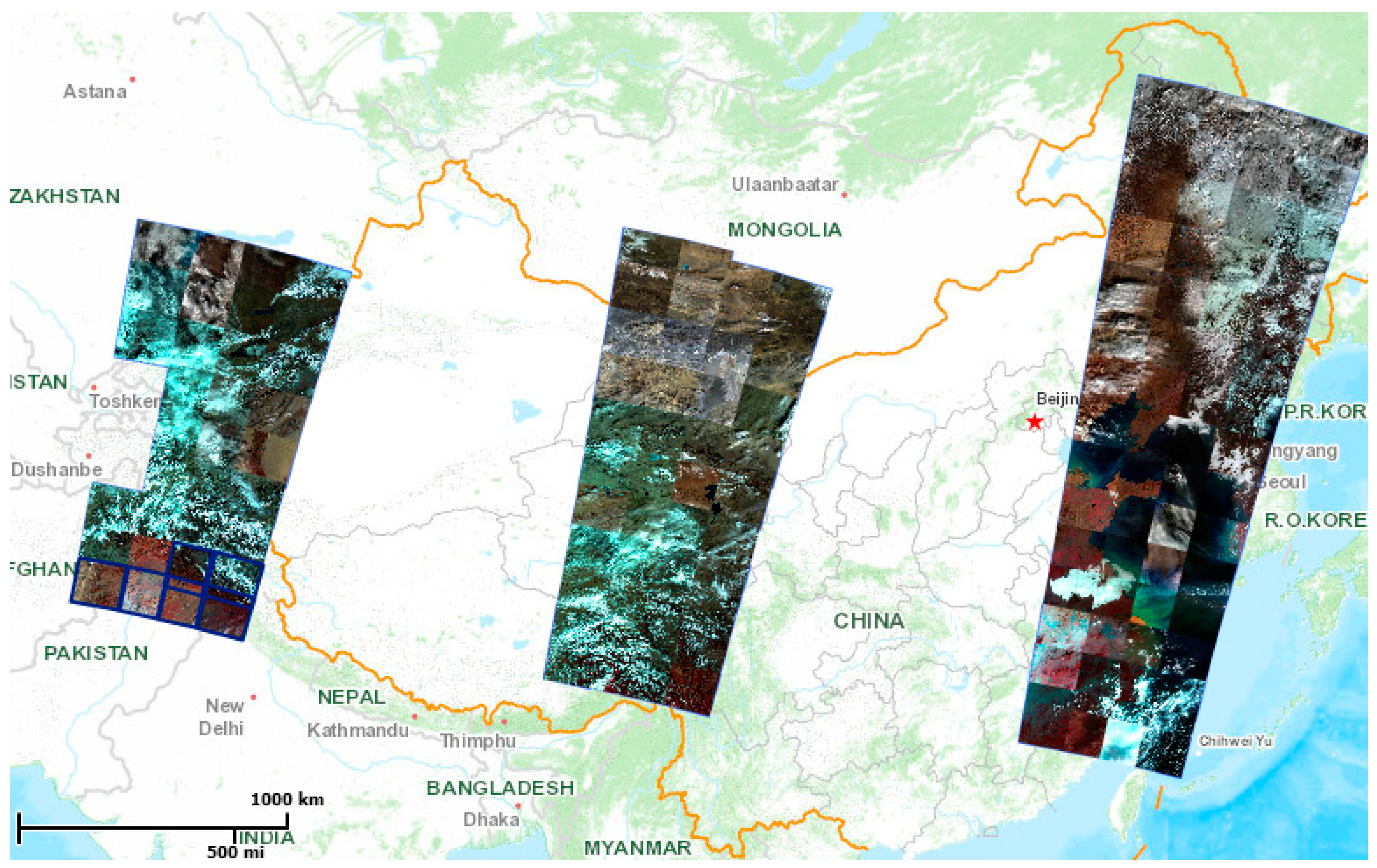
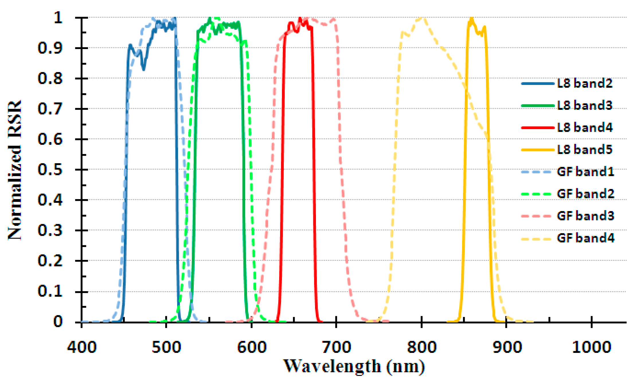
Both Gaofen-1 and Landsat-8 satellites are on sun-synchronous orbits, with an inclination of 98.2°, and their nominal altitudes are 650 km and 705 km, respectively. Similar orbits mean that all the image data over a given location should be collected within 30 min of each other on the same day for the two satellites. Gaofen-1 WFVs are high-resolution push-broom cameras with their spatial resolution of 16 × 24 m (see Table 1). Configured with four cameras, the swath could reach up to ~800 km, resulting in a re-visiting period of four days. Figure 1 shows the footprint of the four cameras in China in a single day, which clearly reveals their superiority in data coverage. There are four spectral bands between visible to NIR, which are quantified over 10-bit digital number (DN). The ground resolution of OLI is 30 m, which is the same as the previous Landsat TM/ETM+ data. The radiometric performance of OLI has been improved with the data quantified in 12-bit. The swath of OLI is 185 km, making the overpass period four times longer than that of Gaofen-1 WFV. The spectral range of the analogous Landsat-8 OLI bands is similar to the WFV, except for a wider bandwidth in NIR (see Table 1). The normalized relative spectral response (RSR) profiles for the two instruments are plotted in Figure 2. In short, Gaofen-1 WFV and Landsat-8 OLI only have small differences in acquisition time within 30 min (see Table 2), band spectral ranges, and ground resolution, thus the well-calibrated OLI appears to be a suitable reference instrument to cross-calibrate WFV observations.

Table 1.
Comparison of the parameters between Gaofen-1 WFV (Wide Field of View) and Landsat-8 OLI (Operational Land Imager).
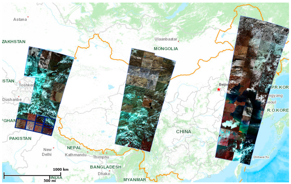
Figure 1.
Footprint of Gaofen-1 WFVs in China in a single day (4-12-2013). With the combination of four cameras on-board Gaofen-1 satellite, the swath of WFV could reach to ~800 km.
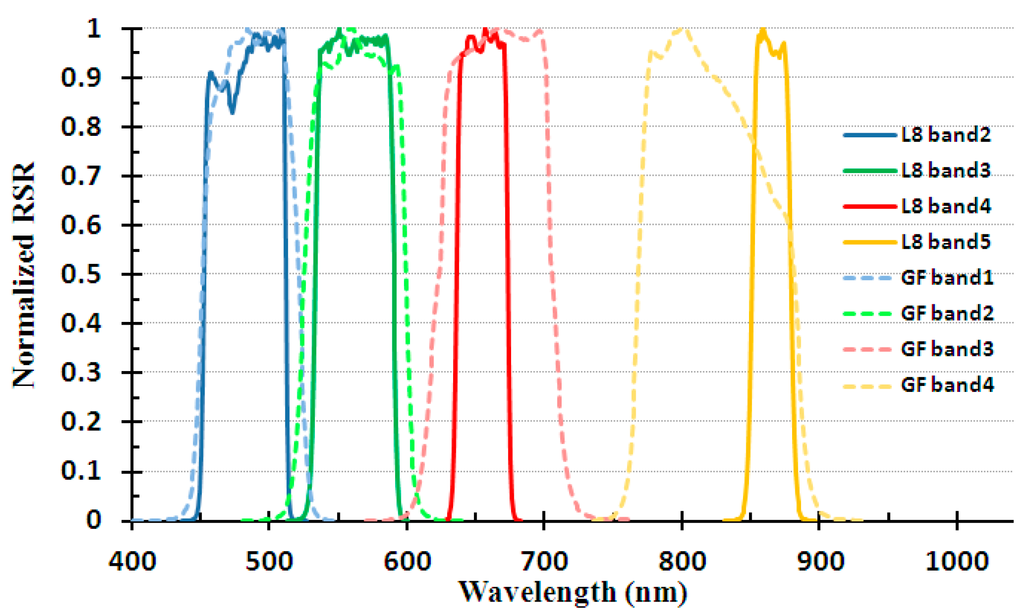
Figure 2.
Comparison of the RSR (Relative Spectral Response) profiles between Gaofen-1 WFV3 and Landsat-8 OLI.
Table 2.
Gaofen-1 WFV3 and Landsat-8 OLI image pairs used in this study.
Landsat-8 OLI and Gaofen-1 WFV3 image pairs with quasi-synchronous acquisition time, large dynamic range (with various surface features) and minimal cloud coverage were selected in this study for both cross calibration and validation. The general information is listed in Table 2. Landsat-8 OLI images were downloaded from United States Geological Survey (USGS, http://glovis.usgs.gov/) and Gaofen-1 WFV data were obtained from CCRSDA (http://www.cresda.com/n16/index.html). To minimize the differences in surface and atmospheric conditions between the observations from reference and target instruments, all WFV–OLI image pairs were acquired within 30 min apart from each other. In addition, visual examinations were conducted to avoid large aerosol changes within these selected image pairs. Changes in sun angle could be corrected with the conversion to TOA reflectance, and a more detailed treatment of the calibration method is given below. Note that reflectance refers to the hemispherical directional reflectance factor (HDRF) throughout this paper [16,17].
The USGS spectral library (splib06a, [18]) was used in this study to correct the potential difference in spectral response caused by different types of surface materials (see details below). The library achieves more than 1300 spectra with spectral range from UV to mid-infrared. The spectral samples were collected from a variety of minerals, plants and manmade materials, assuring that most remotely detected spectral features could find its corresponding spectrum in the library.
3. Method
3.1. Cross Calibration
Remote sensors often respond linearly to the incoming signal. Thus, the quantified standard DNs can be converted to TOA spectral radiance () using the radiance rescaling gains and bias. As for WFV, for a given band ,
where is the band-specific rescaling multiplier and is the band-specific bias. The radiance is then converted to TOA reflectance by
where is the solar zenith angle, is the Earth–Sun distance in Astronomical Units [2], and is the exo-atmospheric solar irradiance (), which can be calculated as follow:
where (non-dimensional) is the normalized spectral response function of the corresponding band, is the continuous exo-atmospheric solar irradiance [19], and are the lower and upper bounds of the spectral range for band .
Meanwhile, the OLI data can be converted to TOA planetary reflectance using reflectance rescaling coefficients provided in the product’s metadata file (MTL file) (http://landsat.usgs.gov/Landsat8_Using_Product.php). The following equation (Equation (4)) is used to convert the quantified and calibrated standard product pixel values () to TOA reflectance with a correction for the sun angle:
where and are the band-specific rescaling multiplier and bias from the metadata, respectively, and is the solar elevation angle.
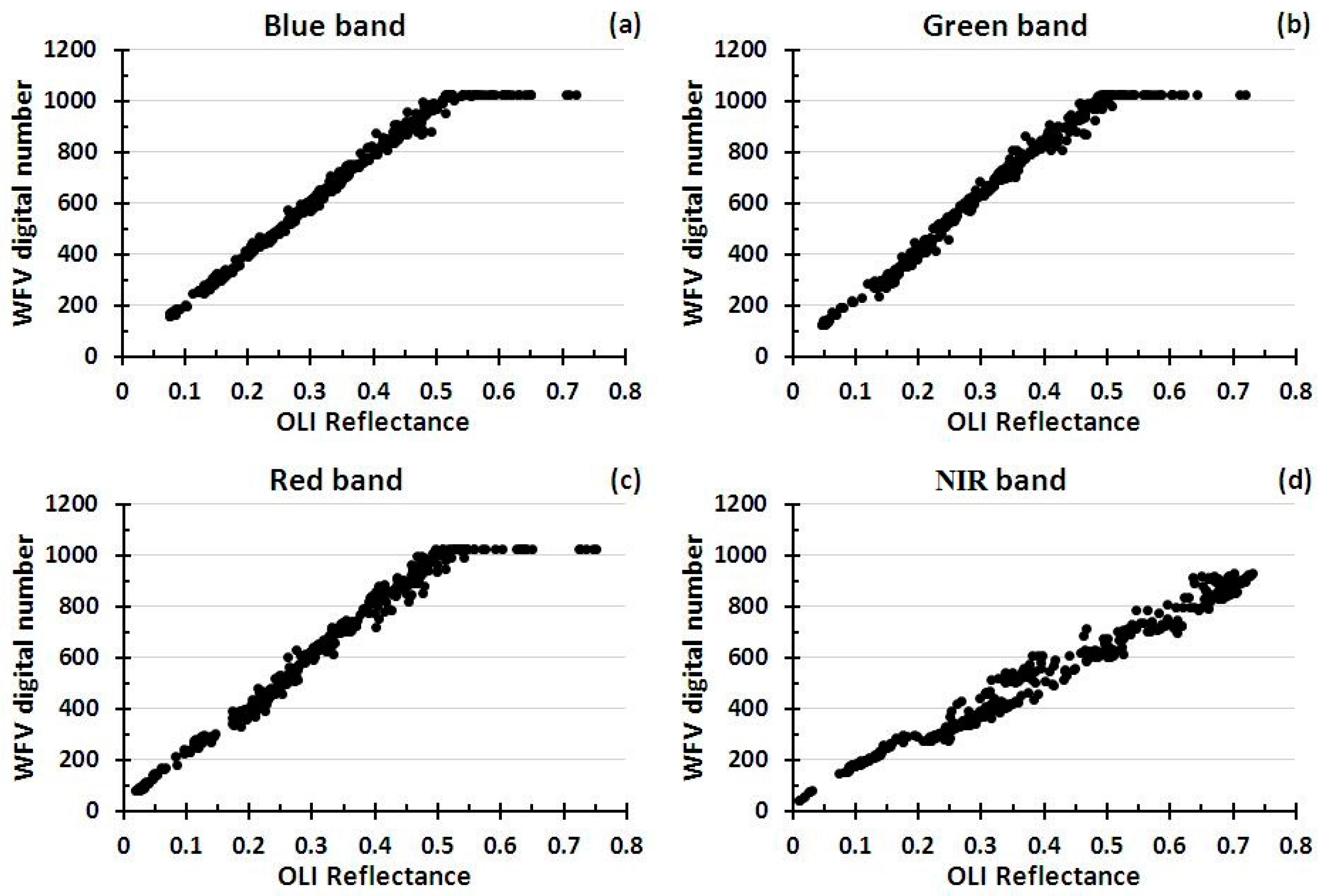
Figure 3 plots the randomly selected Landsat-8 OLI TOA reflectance against Gaofen-1 WFV3 DNs, with each symbol on the plot correspond to mean values of one pair of homogeneous ROIs in the two instruments (see method of ROI selection below). It shows that the WFV3 DNs increase monotonically with the elevated OLI reflectance for the four bands over a wide reflectance coverage (0–0.5). Note that all the image pairs were used to give an objective view for the saturation of the two instruments. The tight linear relationship between WFV3 and OLI signals further confirms the feasibility of using the well performed OLI to cross calibrate the recently launched WFV cameras. Additionally, the results also show that the WFV3 tends to saturate at ~1000 of DN, thus WFV3 data with DN > 1000 were excluded in this study, and the same for other three WFVs.
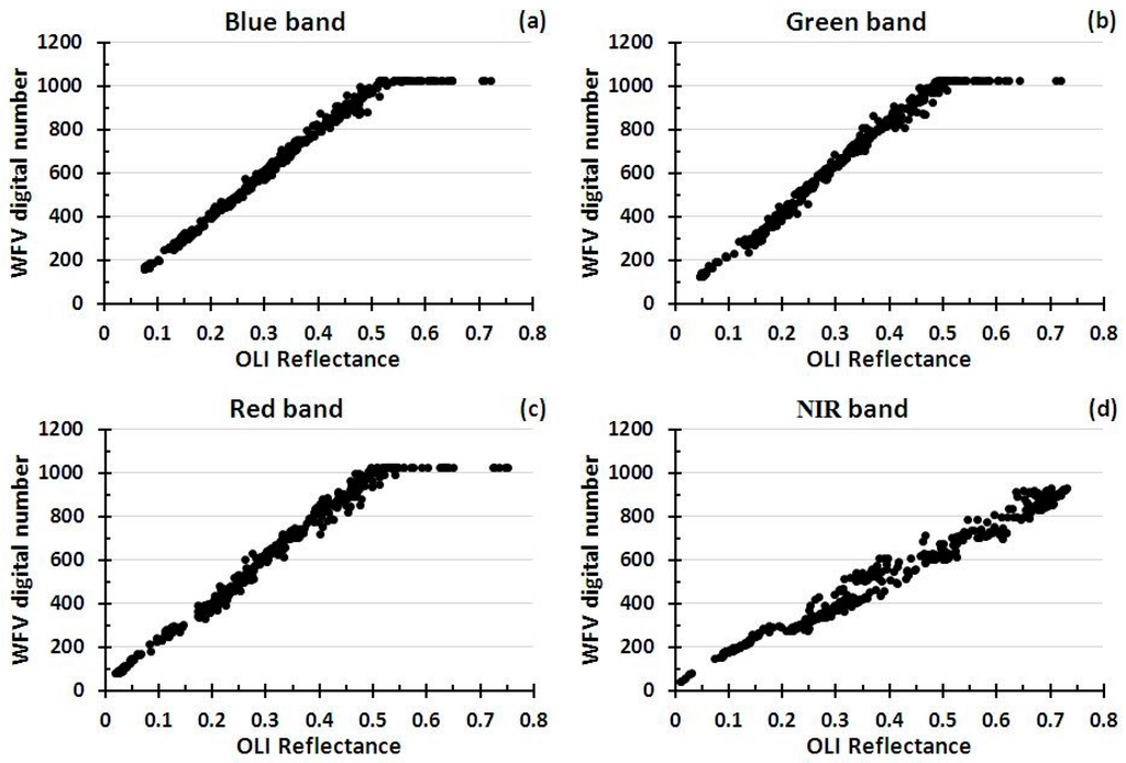
Figure 3.
Landsat-8 OLI reflectance plotted against Gaofen-1 WFV3 digital number (DNs) for the four spectral bands of WFV3: (a) Blue band; (b) Green band; (c) Red band; and (d) NIR band. The WFV3 DNs increases monotonically with the elevated OLI reflectance over a large reflectance coverage (0–0.5). Note that the 10-bit WFV data saturate at ~1000.
Since the data of the two sensors were acquired within 30 min apart, the changes in surface reflectance and the atmospheric conditions were not significant in such a short period. Given the similarity of the spectral bands between the two instruments, the signals received by the target (WFV) and reference sensor (OLI) are the same after accounting for the differences in spectral response, which could be expressed as:
where is the modified TOA reflectance of OLI data, with the spectral and illumination differences between OLI and WFV adjusted; is the spectral band adjustment factor to adjust the differences in relative spectral response profiles and exo-atmospheric solar irradiance between corresponding OLI and WFV spectral bands. The factor varies between different atmospheric transmittances and surface reflectance [12]. With Equations (1)–(4), Equation (5) can be rewritten as:
The objective of cross calibration is to generate calibration coefficients (rescaling gains and offsets ) by using TOA reflectance of Landsat-8 OLI and digital number of Gaofen-1 WFV.
For the reference sensor of OLI, essential coefficients are provided in the metadata file and the DNs can be easily converted to radiance and reflectance. In addition, the information of solar angles is provided in the metadata files of the two types of instruments. Therefore, if the only unknown parameter in Equation (6) is given, calibration coefficients could be obtained using a linear regression between the left side of Equation (6) and digital number of Gaofen-1 WFV on the right side. Thus, to yield cross calibration coefficients for WFV cameras, two critical issues need to be addressed:
- Find sufficient calibration sites (e.g., WFV–OLI matching windows) to establish a statistically meaningful linear fit.
- Determine the spectral band adjustment factor .
3.2. Calibration Sites Selection
The Landsat-8 OLI and Gaofen-1 WFV differ in their along- and across-track pixel sampling. A feature concurrently observed by these sensors is represented by slightly different numbers of image pixels because of the differences in spatial resolution, viewing geometry and sensor scanning times. This makes it difficult to establish direct comparisons on a point-by-point basis. A typical solution is to manually delineate large homogenous areas (or region of interest, ROIs), with the mean statistics of these areas used for both target and reference sensors [12,20,21,22,23]. However, relatively large variations may exist over those visually selected ROIs (say as much as 10 DNs), leading to potential uncertainties in the calibration coefficients. Furthermore, the manual method often suffers from the limitation in data coverage of the two sensors. Thus, an objective and automatic method is proposed in this study to address this challenge. In short, if the coefficient of variation (CV, calculated by standard deviation and mean value, that is stdev/mean) within a window is small enough (<1%), the surface in this window could be considered as homogenous. In practice, a window size of 4 × 3 pixels for OLI image was used, which was close to an area of 5 × 4 window in WFV. The selection of such window sizes is to minimize the variations within the individual windows where the surface changes could be neglected. Additionally, CV with 1% was used as the threshold to determine the potential homogenous regions. The steps of the method are as follows:
- The WFV–OLI image pairs were clipped into the same geographic area with an exclusion of clouds and cloud shadows.
- For each data pair, more than 100,000 random points were generated within the Landsat-8 OLI reflectance image. The random points were based on various combinations of latitudes and longitudes. Then, 4 × 3 windows centered at these points were selected, where the CV were calculated for each window.
- For OLI windows with CV < 1%, the corresponding 5 × 4 windows at the same location were found in the raw WFV image. If the CV for the WFV window is also <1%, the corresponding windows in WFV and OLI were selected as a ROI for further analysis.
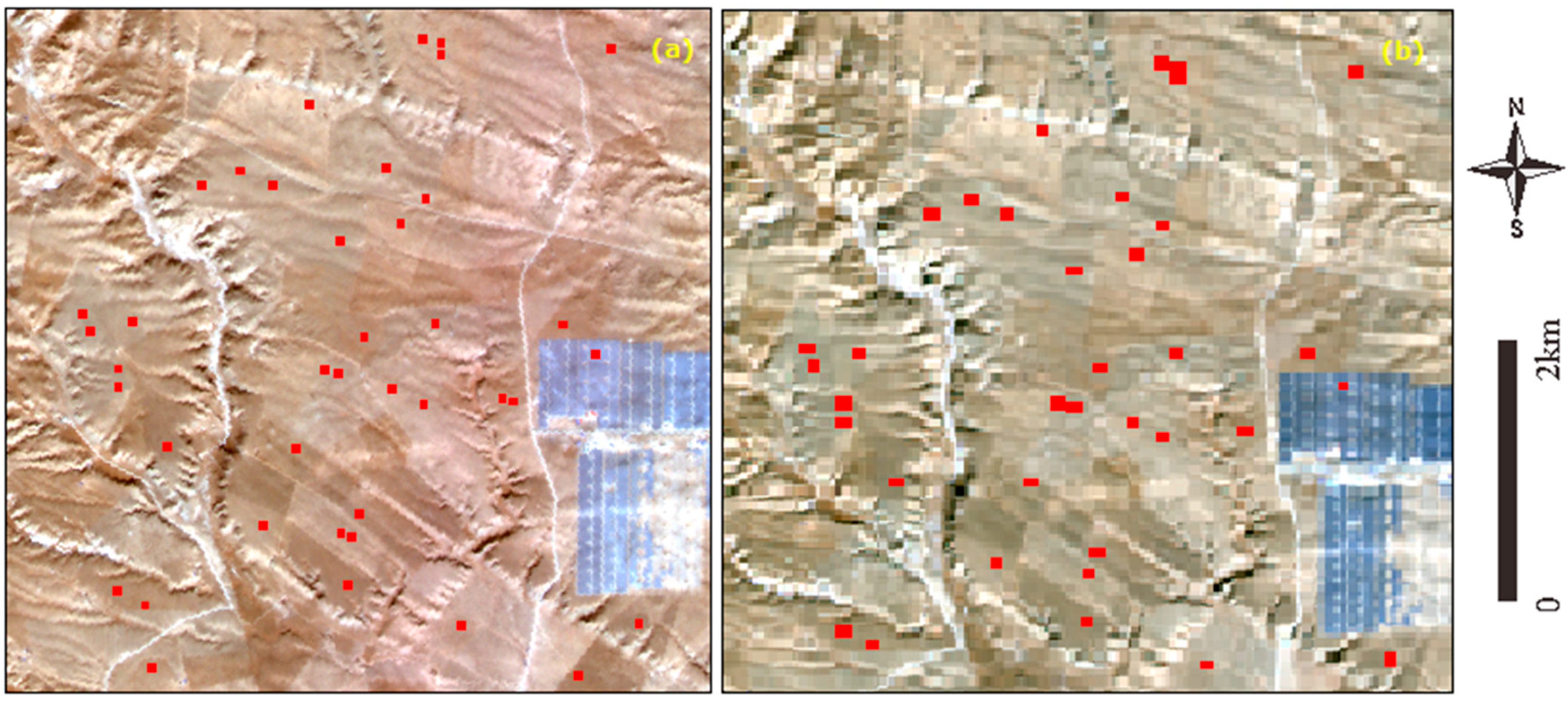
The steps were repeated for four bands of the two instruments (see Figure 4), and for all image pairs used for calibration (see Table 2). The mean values of all the homogenous calibration sites were then estimated for both WFV and OLI images, representing and in Equation (6). A linear regression was conducted to generate calibration coefficients of WFV. As the image pairs covered various surface features, dynamic ranges of the randomly calibration sites (or ROIs) should be sufficient for radiometric calibration.

Figure 4.
An example to show the selected calibration sites (red points) in concurrently collected Gaofen-1 WFV3 (a) and Landsat-8 OLI (b) images.
3.3. Adjustment of the Spectral Band Differences
Figure 2 shows the differences in relative spectral response profiles between corresponding (analogous) spectral bands.
In order to adjust the spectral band differences, first the definition of TOA reflectance is used in cross-calibration. For a given band , reflectance can be defined as:
The only unknown coefficient is the incident continuous spectral reflectance (non-dimensional). Since the incident spectral reflectance of the two sensors is assumed to be the same, the spectral adjustment factor can be defined as:
As normalized spectral response function for the sensors is provided by the manufacturer, the spectral adjustment factor only depends on the incident continuous spectral reflectance .
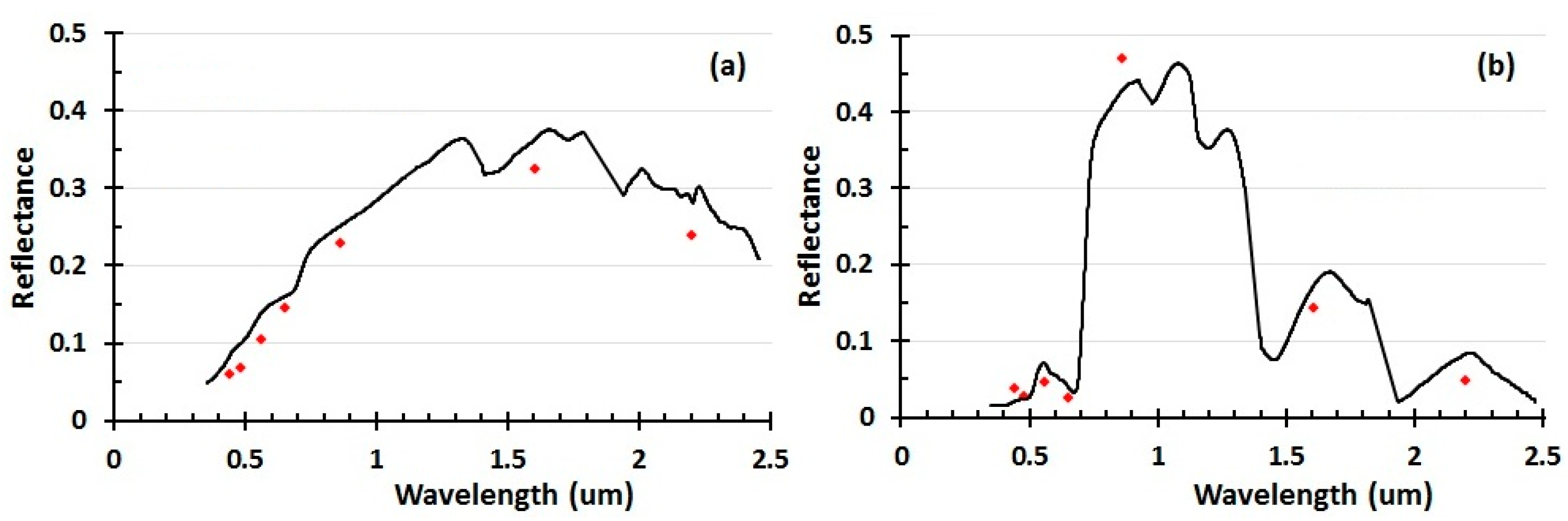
To estimate spectral adjustment factors for different ROIs is not trivial, as changes significantly over different surface conditions, leading to varied for the selected calibration sites. Besides, it seems impossible to obtain accurate for these calibration sites since they were selected randomly. Fortunately, similar spectrum could be found in some of the predefined spectral library, such as the USGS spectral library. After atmospheric correction through FLAASH module in ENVI4.8, the surface reflectance for each Landsat-8 OLI image could be obtained. The key parameters used in the FLAASH module are selected as follows: Mid-Latitude Winter for atmospheric model, Rural for aerosol model (because the selected images is located far away from urban or industrial sources), and 2-Band (K-T) for the aerosol retrieval; the initial visibility was chosen as 20–40 km depending on the image quality. As the hyper-spectral data in the USGS spectral library were collected from numerous surface conditions, the most approximate spectrum can be found to match the atmospherically corrected OLI reflectance correspondingly. In practice, minimum mahalanobis distance was used to determine the similarity between the OLI reflectance and continuous spectral data in the library. Figure 5 demonstrates two typical examples of the matched OLI reflectance (points) and hyper-spectral data (curves) of the USGS library for different surface types. The spectral shapes and magnitudes between the two different measurements are close to each other, suggesting that the hyper-spectral data matches very well to the OLI reflectance, which could be used to calculate the spectral adjustment factors for the corresponding OLI pixels. As such, for all of the selected calibration sites could be estimated using the above method. It should be noted that the only purpose of the atmospheric correction for OLI images was spectrum matching, and the input of the cross calibration equation in Equation (6) is TOA reflectance.
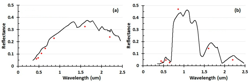
Figure 5.
Examples to show the mean reflectance of atmospherically corrected Landsat-8 OLI (red points) in two ROIs and their matched spectrum in the USGS spectral library (curves): (a) desert; and (b) vegetation.
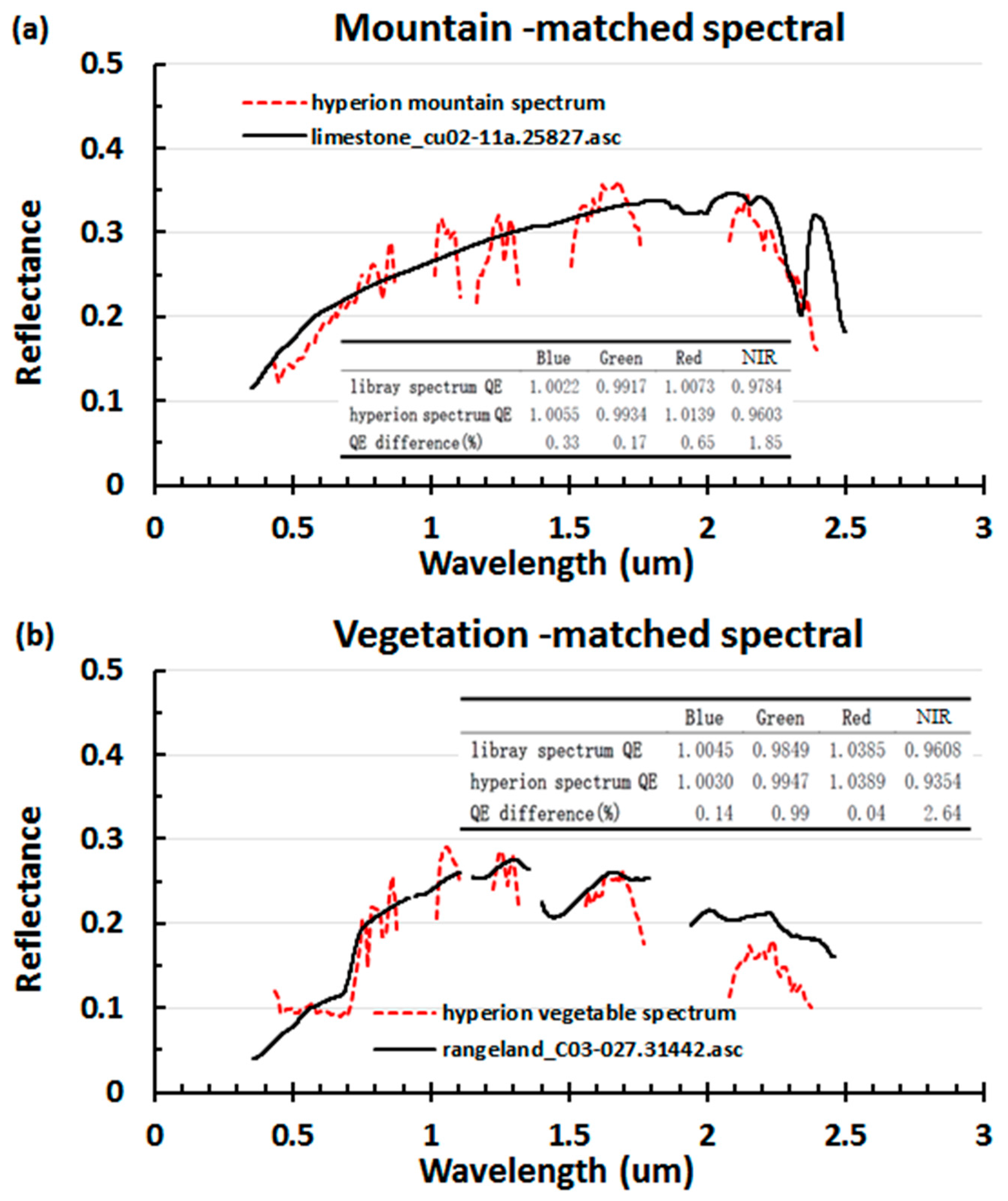
Theoretically, simultaneously measured in situ hyper-spectral data or hyperspectral images (such as Hyperion) should be used to calculate [24,25]. While in practice, to obtain sufficient concurrent spectral measurements for randomly selected calibration sites of a large coverage is very difficult. As a solution in this study, atmospherically corrected surface reflectance of Landsat-8 OLI was used to find the “most approximate” hyperspectral data in the USGS spectral library, with which the can be calculated. In order to do the atmospheric correction, the MODTRAN4 radiation transfer code incorporated in FLAASH module of ENVI4.8 software was used, which is considered to be a good solution for atmospheric corrections for terrestrial applications [26]. As long as the spectral shape is similar, the spectral matching and estimation should be immune to the residual errors caused by atmospheric correction. In addition, the accuracy of the USGS-estimated can be partially validated with sporadic Hyperion images. Concurrently collected OLI and Hyperion images were downloaded and ROIs with CV < 1% in the OLI image were selected. Then, the corresponding could be estimated using either the matched USGS spectral library or the geo-matched Hyperion data. As for two typical surface features (see Figure 6), the spectral shapes are similar for the two independent measurements (USGS library and Hyperion), and the differences between the two are <1% for blue to red bands and <3% for NIR bands, respectively. ROIs of other surface types also show similar results, suggesting that the use of USGS spectral library in this study is valid.
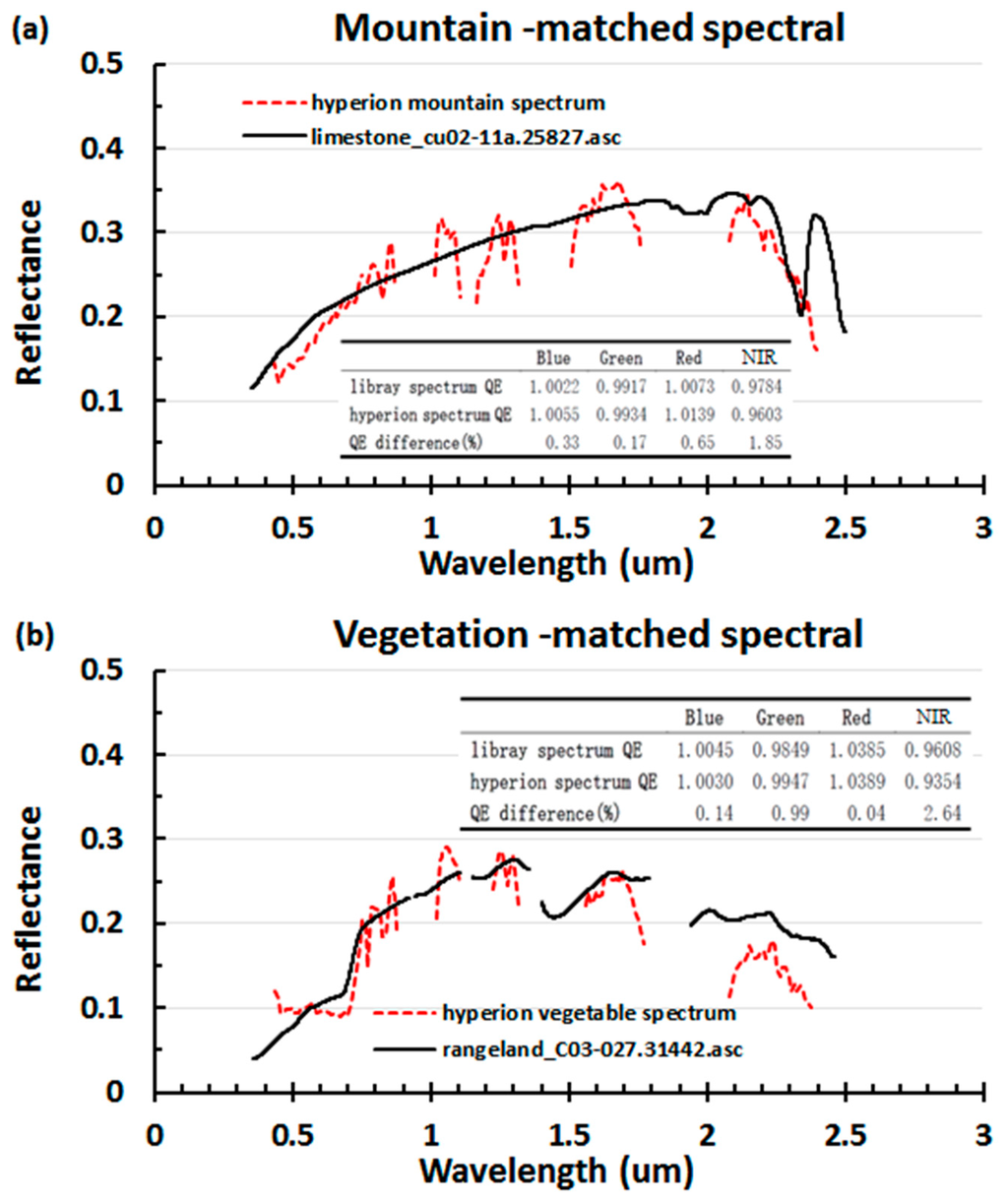
Figure 6.
The comparisons between the ROI matched spectrum in the USGS library and those of from the concurrently collected Hyperion image for two typical surface features, (a) for mountain; and (b) for vegetation, respectively.
4. Results and Validations
4.1. Results of cross Calibration
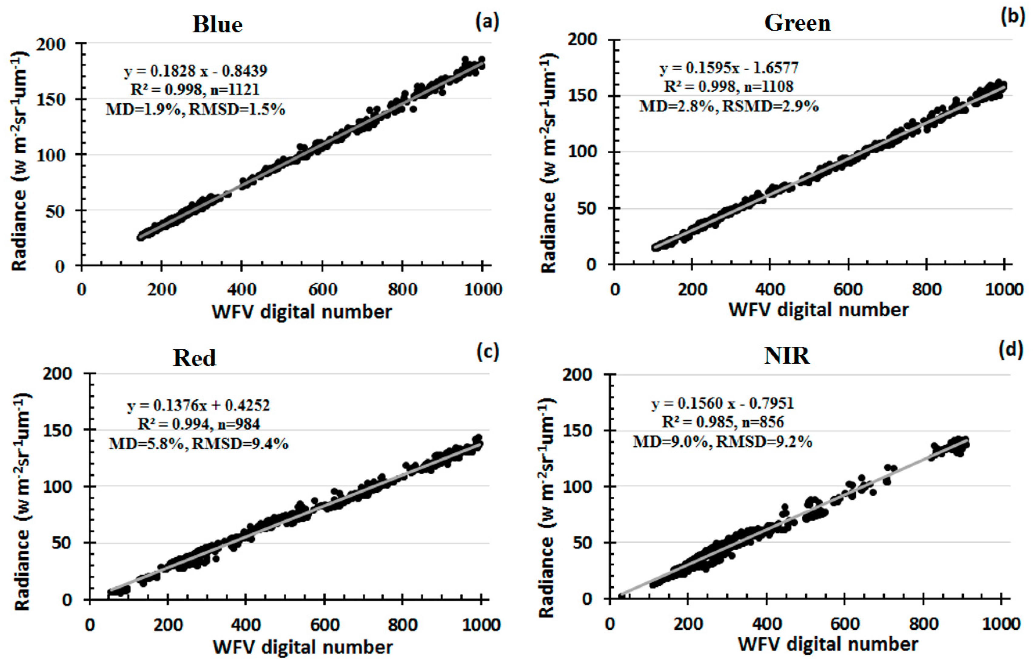
With sufficient calibration sites (from all five selected image pairs, see Table 2) and close estimates of spectral adjustment factors, a linear regression based on Equation (6) could yield cross calibration coefficients (both gains and offsets) for Gaofen-1 WFV cameras. Figure 7 plots the left side of Equation (6) (or adjusted OLI radiance) and DNs of WFV3 for all four spectral bands. Within a large dynamic range, the >800 points for each band are aligned along the fitting line, suggesting that the performance of the linear fits are satisfactory and the regression coefficients should be valid. Tests of the hypothesis of zero gain and offset has been rejected for all the bands (using SPSS software), with a significant level of <0.01. Additionally, the mean relative difference (MD) and root mean square root mean difference (RMSD) between the linear relations estimated radiance using DN of WFV and the adjusted OLI radiance were very small for each band (see Figure 7). Note that, when randomly selecting half of the points, the produced coefficients were almost identical to the current form.
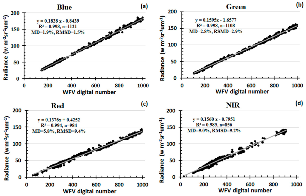
Figure 7.
TOA radiance of selected calibration sites from Landsat-8 OLI plotted against the digital number of Gaofen-1 WFV3: (a) Blue band; (b) Green band; (c) Red band; and (d) NIR band. Linear fits between them resulted in cross calibration coefficients for the WFV instrument. Note that the RSR differences between the two sensors were adjusted.
Using the same cross calibration method of WFV3, the radiometric calibration coefficients for the other three WFV cameras (WFV1, WFV2 and WFV4) were also generated. Table 3 compares the officially provided (old) and the newly-generated (new) gains and offsets for all of the four WFV instruments, with the differences between the two sets of calibration coefficients evaluated. Generally, the cross-calibrated gains in green and red bands show small differences to the old gains, with <6% differences for four cameras and almost identical gains for WFV1. However, large discrepancies could still be observed in blue and NIR bands. The blue band shows new/old gain ratios of 1.16 for WFV2 and 1.17 for WFV3, respectively, and ratio of 1.15 is observed in the NIR band of WFV4. Furthermore, the ratio for NIR band of WFV2 even reached 1.41.
Table 3.
Cross-calibrated gains and offsets (new) for four WFV sensors of Gaofen-1 satellites, also listed are the officially provided calibration coefficients (old). Differences between the two sets of calibration coefficients were calculated.
In addition, large differences exist between the officially provided offset and that of the re-calibrated, which can be observed in almost all spectral bands for the four WFV instruments. Table 3 lists the differences between the new and the old offsets (see column “Difference”), and the corresponding digital numbers are also calculated (Difference/new gain). The absolute values of old gains appear to be much larger than their cross-calibrated counterparts across different spectral bands and instruments. For example, the old offset of the red band in WFV2 is 15.3820 () larger than the newly-yielded offset, corresponding to 80.4 digital counts when the new gain is used. Overall, the offset differences were generally larger than 15 DNs, with only two exceptions in blue (1.9 DNs) and red (5.0 DNs) bands of WFV1, respectively.
4.2. Validations
Concurrent radiometrically calibrated TOA reflectance of Landsat 8 OLI images, after correction of the spectral response difference with WFV, was considered as the ground truth to validate the performance of the newly-produced calibration coefficients. Note that the image pairs for validation are not the same as that were used for cross calibration (see Table 2), and the surface and atmospheric conditions were assumed the same for each images pairs.
To calculate the difference between the cross-calibrated Gaofen-1 WFV3 and Landsat-8 OLI reflectance in a statistically meaningful way, over 1000 random points from concurrent WFV–OLI image pairs were selected. Then the difference (in percentage) of the reflectance between the two sensors was calculated for each point, and the accuracy statistics were based on the results of all the random selected points. Figure 8 plots the mean differences and their associated standard deviations for different reflectance ranges of the four spectral bands. For comparison, the differences between WFV3 reflectance calibrated with official (old) coefficients and OLI reflectance are also plotted in Figure 8. The detailed data are listed in Table 4.
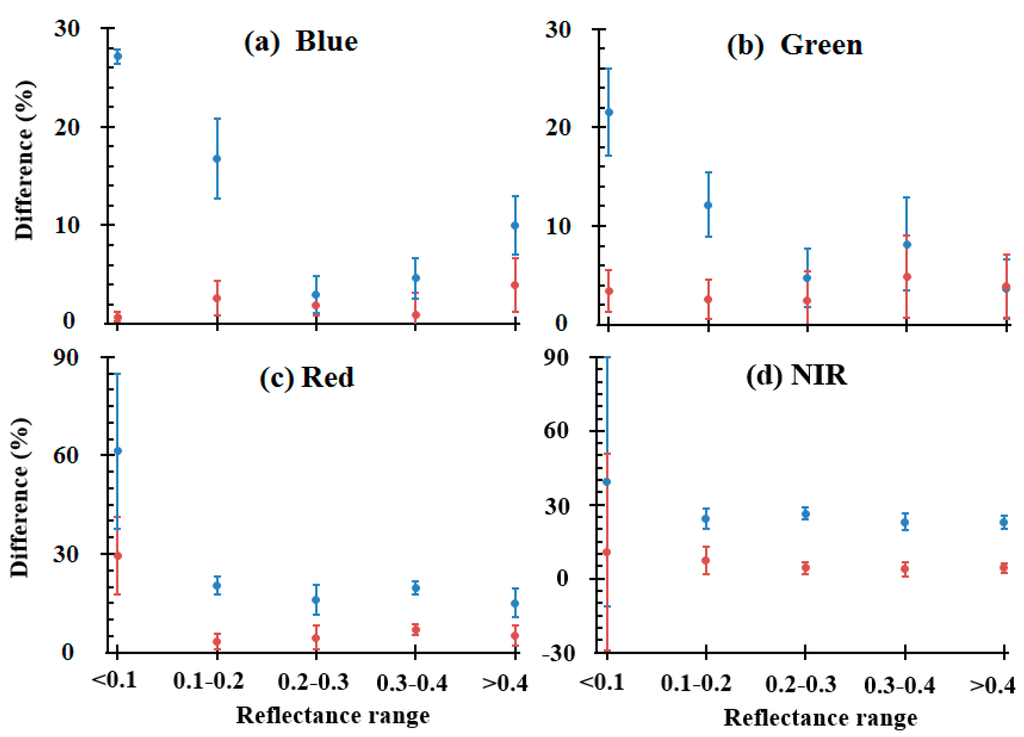
Figure 8.
Differences between the cross calibrated WFV3 reflectance and radiometrically calibrated Landsat-8 OLI data for different reflectance ranges of four bands (in red, points and bars represent mean and standard deviation, respectively): (a) Blue band; (b) Green band; (c) Red band; and (d) NIR band. For comparison, the differences using the officially provided calibration coefficients of WFV cameras were also plotted (in blue). The RSR differences between the two sensors were adjusted.
Table 4.
The differences between the radiometrically calibrated Landsat-8 OLI and WFV3 reflectance in different reflectance ranges, the calculations were conducted using both new and old calibration coefficients of WFV3. The last column estimated the improvements of WFV3 after cross calibration. Note that the RSR differences between the two sensors were adjusted.
The cross-calibrated reflectance agrees very well with the OLI reflectance, with the mean differences between the two sensors <5% for most of the reflectance ranges of the four spectral bands. Since the radiometric calibration error of Landsat-8 OLI reflectance is <3% [14], the uncertainty of the newly-calibrated WFV reflectance should be within 8%. When compared with the results of the old calibration coefficients, the improvements are between 1% and 26% for difference bands and reflectance ranges, and the overall improvement of the cross calibration is 13.67% for all four spectral bands. However, the differences and standard deviations at low reflectance (0–0.1) of red and NIR bands are relatively larger than other bands. The surface type associates with low reflectance in red and NIR bands is likely to be water, as the water absorbs most of the solar radiances in these spectral ranges [27]. The radiance interactions with the air and water surface were not considered in this study, which may explain the large discrepancies in these two bands. Additional water-target based cross calibration method is required to improve the performance in the low reflectance ranges of the two bands [28]. In addition, half of the validation points were randomly selected, and the uncertainty estimates were very similar to the current form.
To visualize the improvements of cross calibration, four-band spectrum from typical surface features are plotted (Figure 9). For water surface, large gaps can be observed in all of the four spectral bands between WFV reflectance calibrated with official coefficients and OLI reflectance. In contrast, WFV reflectance calibrated with new coefficients appears to be much closer to OLI reflectance in terms of both spectral shapes and magnitudes. The reflectance of vegetation and desert using new coefficients is also much closer to the OLI reflectance, suggesting that WFV cameras are able to have similar observations as OLI when the new calibration coefficients are applied.
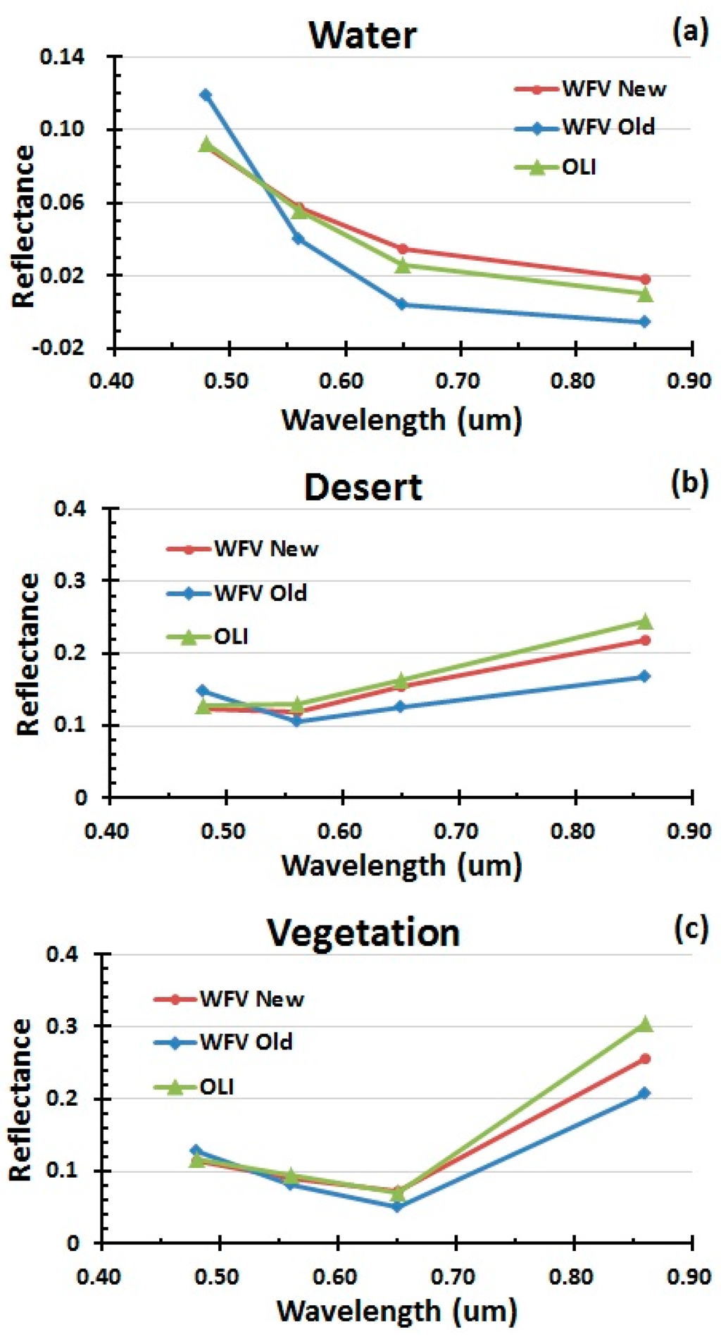
Figure 9.
Comparison of the reflectance between Landsat 8 OLI and Gaofen-1 WFV under typical surface conditions: (a) water; (b) desert; and (c) vegetation. Both cross calibrated (new) and officially coefficients calibrated (old) WFV reflectance were plotted. The cross calibrated WFV agreed much better with the OLI reflectance.
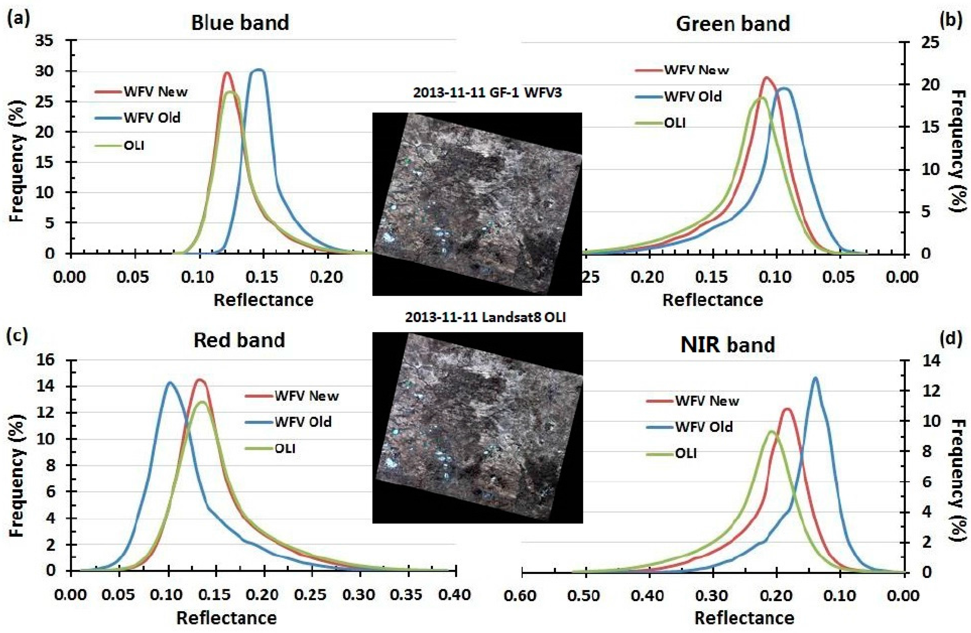
To further validate the reflectance distributions of the cross-calibration coefficients, reflectance histograms for different bands of one typical OLI-WFV image pair were generated. Figure 10 shows the histogram comparisons for the four bands. Similar to the point-to-point and typical surface feature comparisons, differences between WFV and OLI has considerably decreased when new calibration coefficients are used, with the reflectance histograms matching very well in blue to red bands. Nevertheless, the relative larger uncertainties of the cross-calibration coefficients at the low reflectance range (see above analysis and Figure 8) may have led to the mismatched histogram in NIR band.
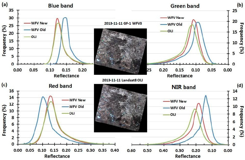
Figure 10.
Comparison of the reflectance histograms in one WFV–OLI image pair for four bands: (a) Blue band; (b) Green band; (c) Red band; and (d) NIR band. Both cross calibrated (new) and officially calibrated (old) WFV reflectance were included.
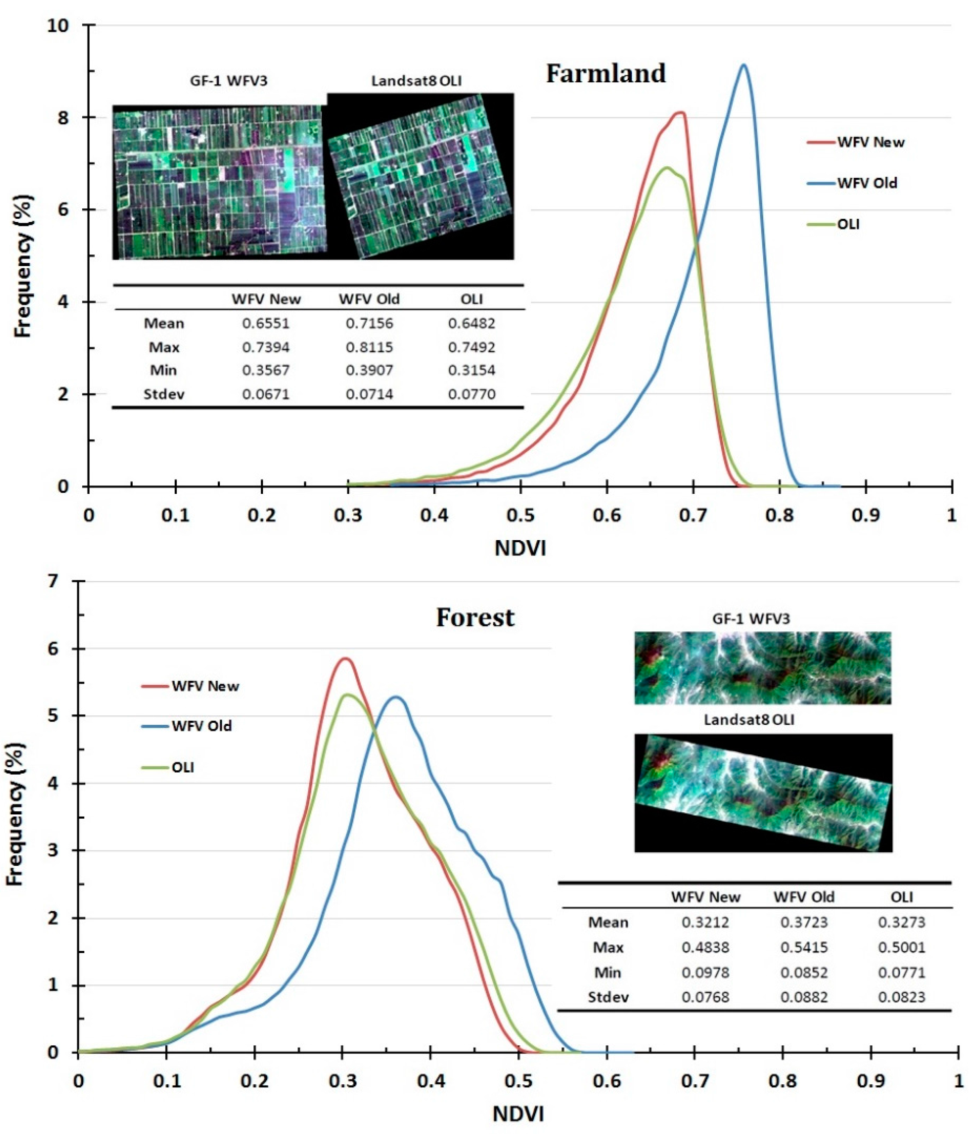
To explore the application of the cross-calibration results, Normalized Difference Vegetation Index (NDVI) of Gaofen-1 WFV camera were validated, where ( is the TOA reflectance [12]). Figure 11 compares the histograms and statistics of NDVI for WFV and OLI in farmland and forest, where both new and old calibration results of WFV are included. Clearly, NDVI results using newly-calibrated coefficients are more consistent with the OLI than those calculated with the officially provided coefficients (see Figure 11), and the statistics (including maximum, minimum and mean values) and histograms are much closer to the Landsat-8 OLI estimates for the two different types of vegetation.

Figure 11.
Comparison of the histograms and statistics of NDVI for WFV and OLI in typical farmland and forest, where both cross calibrated (new) and officially calibrated data (old) for WFV were calculated.
5. Discussion
With data collected by Landsat-8 OLI as reference, Gaofen-1 WFV instruments were re-calibrated using a novel cross calibration scheme. The reflectance estimated using the officially provided calibration coefficients showed large differences from the concurrent OLI images. In comparison, the radiometric performance of the cross-calibrated WFV cameras has improved significantly, as the spectral shapes, reflectance magnitudes and distributions, as well as the estimated vegetation index (NDVI) agreed very well with those of the tandem Landsat-8 OLI measurements. We attribute the success of the cross-calibration to two factors: (1) An objective method to select sufficient homogenous calibration sites, where good linear regressions could be established with large dynamic ranges; (2) Continuous hyper-spectral data in the USGS spectral library used to estimate the factors to adjust differences in the relative spectral response profiles between the reference and target sensors.
To guarantee the homogeneity of the selected calibration sites, a small window size of 4 × 3 pixels for Landsat-8 OLI was used to geo-match the window in WFV images to assure minimal variations within each site, as a larger window could result in a higher likelihood of with-in site heterogeneity, which could propagate into the cross calibration coefficients. The threshold of 1% for CV was a compromise between the uncertainties of linear regressions and the number of calibration sites, as smaller thresholds could result in less data coverage, and larger values often lead to more potential uncertainties. To test the rationality of the use of 1% [29], Gaussian noise with a standard deviation of 1% were added to the selected sites for both OLI and WFV instruments. Results show that the difference of each band between the noise-added and the presented coefficients were within 0.3% for gain and <0.15 for offset, respectively, suggesting that the uncertainty resulted from the 1% CV criteria can be ignored.
Although the spectral ranges of Gaofen-1 WFV cameras are similar to the analogous wavelengths of Lansat-8 OLI (especially for the blue and green bands, see Table 1), the relative spectral response varies, resulting in different reflectance even for the same target between the two sensors. Thus, the correction of RSR differences appears to be a critical step in the cross calibration method. Using the USGS spectral library, we estimated the ranges of RSR adjustment factors () for different types of surface features, where the data were classified (or chartered) following same convention of the USGS library. The range of changes significantly among different surface types and spectral bands, with the maximum and minimum values observed in the red (0.8908) and green (1.3929), respectively (Table 5). In other words, the reflectance differences for the same target observed by the two sensors could reach ~40%, suggesting the crucial role of RSR adjustments in cross calibration between OLI and WFV instruments.
Table 5.
The range of RSR adjustment factors for different surface features, which were estimated using the USGS spectral library, the chapters were followed the same convention of the library.
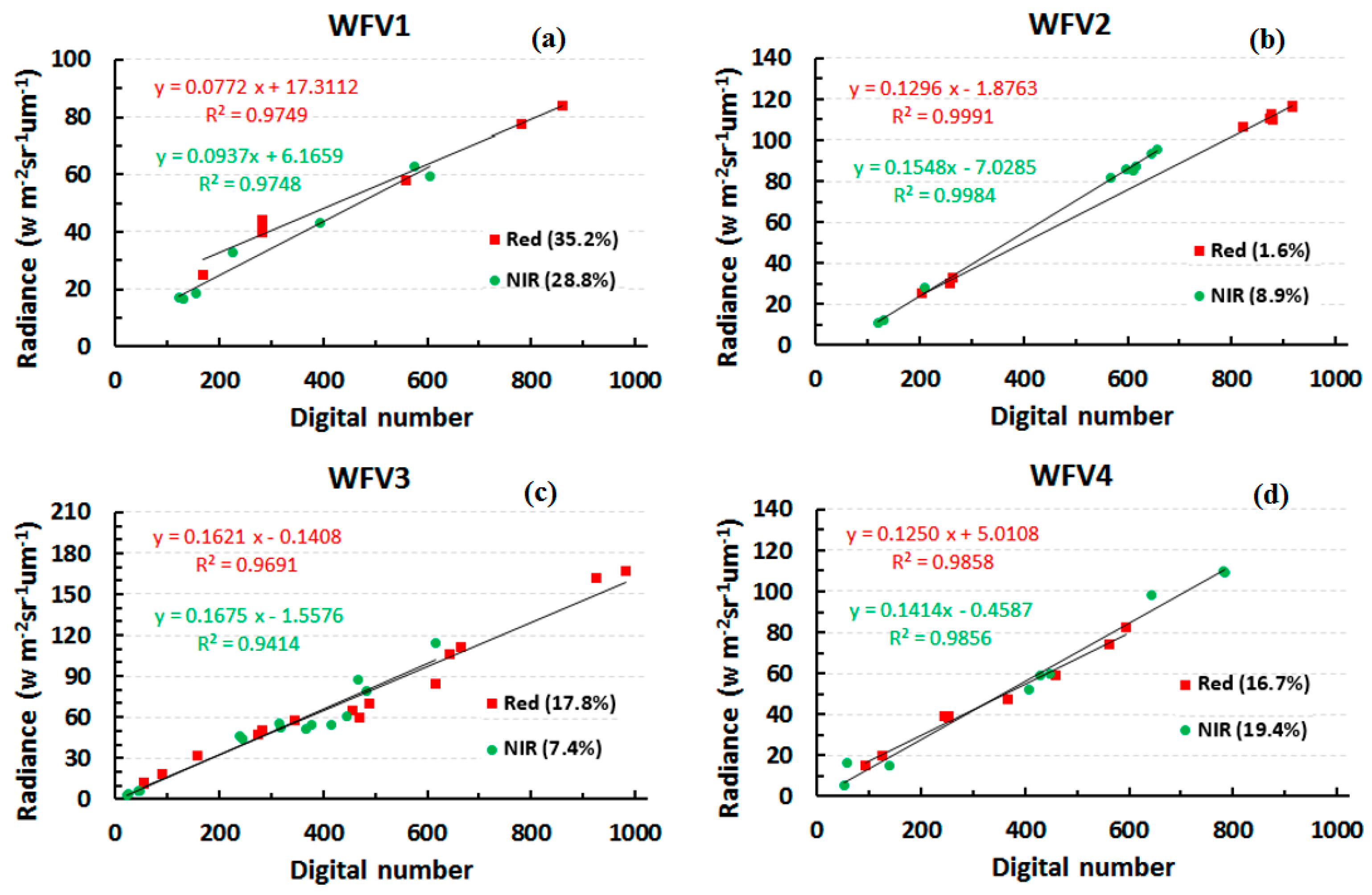
Why was Landsat-8 OLI selected as the reference rather than other accurately calibrated instruments? For example, MODIS instruments (Terra and Aqua) have demonstrated stable calibrations over the last decades [3], and have similar spectral bands with those of WFV. However, the one order of differences in the ground resolutions (250–500 m for MODIS) may lead to potential uncertainties to the calibration results. To compare, the two 250 m MODIS bands (red and NIR) were also used to cross calibrate the analogues WFV bands, where the ROIs were manually selected following the similar method as described by Chander et al. [10] and the differences in spectral responses were also adjusted with the USGS spectral library. As shown in Figure 12, although the performance of the linear regressions is acceptable for all of the four WFV sensors, the differences in gains between the MODIS- and OLI-derived coefficients appear to be too large. The differences in gains for the red and NIR bands between the two methods even reach up to >30% for a certain WFV band. Given the accurate calibration of the OLI data [15] and the high agreement of its cross calibrated WFV reflectance (differences <5% for any given bands, see Figure 8 and Table 4), the calibration coefficients with MODIS are likely to be problematic.
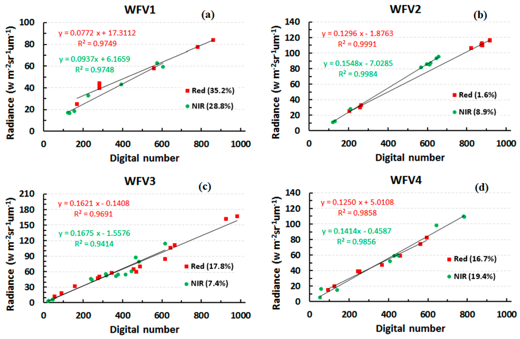
Figure 12.
Cross calibration results using Moderate Resolution Imaging Spectroradiometer (MODIS) 250 m bands, where the homogenous ROIs were manually selected and the differences in spectral responses were adjusted. The differences between the MODIS- and OLI-cross calibrated gains (in percentage) for each band are also shown in the parentheses. (a) WFV1; (b) WFVV2; (c) WFVV3; (d) WFVV4.
For the predecessors of Landsat ETM+, the SLC failures will lead to difficulties in ROI selection. Moreover, the mission has exceeded its designed life (5 years) and can terminate at any time, thus the newly-launched OLI appears to be more appropriate as it can be used in the future for radiometric degradation correction of WFVs. The Gaofen-1 WFV cameras have already been collecting data for nearly three years, yet optical remote sensors often suffer from signal degradations after a certain period of operation [30]. The method in this study can be used frequently to monitor and correct the potential reflectance biases caused by sensor degradation of WFV cameras, as long as a stable reference data can be obtained. This is particularly true for the instruments on-board Landsat series satellites [5]. Furthermore, the Chinese government has approved CHEOS to continue launching another four or five satellites as complementary missions for Gaofen-1 [31]. The proposed method here can be used in the future to provide accurate and consistent observations for these planned missions.
Of the four WFV cameras onboard Gaofen-1 satellite, two of them are close-nadir view (WFV2 and WFV3) and the other two are of off-nadir view (WFV1 and WFV4). The large view angle of the two latter instruments may lead to relatively longer atmospheric path and thus larger path radiance than the OLI. When the view angle increase from 0° to 40°, the atmospheric path radiance can increase by 15%~30% depending on the different aerosol conditions [32]. Additionally, many bi-directional effects may also occur with large sensor zenith angles. Therefore, the uncertainty of the calibration coefficients derived for WFV1 and WFV4 in this study could be larger than the other two close-nadir instruments, and a more sophisticated method is required to solve the large view angle associated problems [32].
6. Conclusions
A simple cross calibration method has been proposed and implemented to radiometrically cross calibrate the Gaofen-1 WFV cameras using simultaneously collected Landsat-8 OLI data. An objective method was proposed to select sufficient homogeneous calibration sites with a large dynamic coverage for both the reference and target instruments. Then, the atmospherically corrected OLI reflectance for each calibration site was used to match the hyper-spectral data in USGS spectral library. The adjustment factor estimated by the matched spectrum was then used to correct the spectral band (or response) differences between the two sensors. Compared with the officially provided coefficients, the performance of the cross calibrated coefficients improved significantly. The newly calibrated reflectance showed small difference (<5%) with the calibrated OLI reflectance for the four spectral bands over a large reflectance range. Similar consistencies between the cross-calibrated WFV and OLI were also found for their reflectance distributions and vegetation index statistics. Considering the ~3% calibration uncertainty of OLI, the errors of the newly-calibrated WFV reflectance (at least for close-nadir instruments) should be within 8%. Although with much improvements over the original coefficients, more sophisticated method and thus higher calibration accuracy may be required for quantitative remote sensing applications in the future.
Landsat series of satellites have been providing consistent long term global observations, and on-board and vicarious calibrations for these instruments are performed constantly to guarantee their high accuracy in radiometric calibration. Because of availability of Landsat data, the approach developed here can be easily extended to future satellite missions of China or other countries to obtain valid radiometric calibration coefficients.
Acknowledgments
This work was supported by the National Natural Science Foundation of China (NO. 41401388, 41571344, 41576175, and 41301463) and the Fundamental Research Funds for the Central Universities and the open-fund projects of LIESMARS (Wuhan University). We thank the USGS for providing Landsat data and spectral library.
Author Contributions
Juan Li carried out most of the data processing and prepared the manuscript draft; Lian Feng came up with the idea and helped organized the research; Xiaoping Pang and Xi Zhao helped to outline the manuscript structure; and Weishu Gong helped to prepare the manuscript.
Conflicts of Interest
The authors declare no conflict of interest.
References
- Hu, X.; Liu, J.; Sun, L.; Rong, Z.; Li, Y.; Zhang, Y.; Zheng, Z.; Wu, R.; Zhang, L.; Gu, X. Characterization of CRCS Dunhuang test site and vicarious calibration utilization for Fengyun (FY) series sensors. Can. J. Remote Sens. 2010, 36, 566–582. [Google Scholar] [CrossRef]
- Chander, G.; Markham, B.L.; Helder, D.L. Summary of current radiometric calibration coefficients for Landsat MSS, TM, ETM+, and EO-1 Ali sensors. Remote Sens. Environ. 2009, 113, 893–903. [Google Scholar] [CrossRef]
- Xiong, X.; Barnes, W. An overview of MODIS radiometric calibration and characterization. Adv. Atmos. Sci. 2006, 23, 69–79. [Google Scholar] [CrossRef]
- Hu, Z.; Ge, G.; Liu, C.; Chen, F.; Li, S. Structure of Poyang lake wetland plants ecosystem and influence of lake water level for the structure. Resour. Environ. Yangtze Basin 2010, 19, 597–605. [Google Scholar]
- Gregg, W.W.; Casey, N.W. Global and regional evaluation of the SeaWiFS chlorophyll data set. Remote Sens. Environ. 2004, 93, 463–479. [Google Scholar] [CrossRef]
- Han, X.; Chen, X.; Feng, L. Four decades of winter wetland changes in Poyang lake based on Landsat observations between 1973 and 2013. Remote Sens. Environ. 2015, 156, 426–437. [Google Scholar] [CrossRef]
- Feng, L.; Hu, C.; Chen, X.; Zhao, X. Dramatic inundation changes of China’s two largest freshwater lakes linked to the Three Gorges Dam. Environm. Sci. Technol. 2013, 47, 9628–9634. [Google Scholar] [CrossRef] [PubMed]
- Lawrence, M.G. The relationship between relative humidity and the dewpoint temperature in moist air: A simple conversion and applications. Bull. Am. Meteorol. Soc. 2005, 86, 225–233. [Google Scholar] [CrossRef]
- Hooker, S.B.; Esaias, W.E.; Feldman, G.C.; Gregg, W.W.; McClain, C.R. An Overview of SeaWiFS and Ocean Color; National Aeronautics and Space Administration, Goddard Space Flight Center: Greenbelt, MD, USA, 1992. [Google Scholar]
- Chander, G.; Meyer, D.J.; Helder, D.L. Cross calibration of the Landsat-7 ETM+ and EO-1 Ali sensor. IEEE Trans. Geosci. Remote Sens. 2004, 42, 2821–2831. [Google Scholar] [CrossRef]
- Shang, G.-P.; Shang, J.-C. Causes and control countermeasures of eutrophication in Chaohu lake, China. Chin. Geogr. Sci. 2005, 15, 348–354. [Google Scholar] [CrossRef]
- Teillet, P.; Barker, J.; Markham, B.; Irish, R.; Fedosejevs, G.; Storey, J. Radiometric cross-calibration of the Landsat-7 ETM+ and Landsat-5 TM sensors based on tandem data sets. Remote Sens. Environ. 2001, 78, 39–54. [Google Scholar] [CrossRef]
- Yang, G.; Ma, R.; Zhang, L.; Jiang, J.; Wei, S.; Zhang, M.; Zeng, H. Lake status, major problems and protection strategy in China. J. Lake Sci. 2010, 22, 799–810. [Google Scholar]
- Doerffer, R.; Schiller, H. The MERIS case 2 water algorithm. Int. J. Remote Sens. 2007, 28, 517–535. [Google Scholar] [CrossRef]
- Barsi, J.A.; Markham, B.L. Early Radiometric Performance Assessment of the Landsat-8 Operational Land Imager (OLI). In Proceedings of the SPIE Optical Engineering + Applications; International Society for Optics and Photonics, San Diego, CA, USA, 26–29 AUG 2013.
- Odongo, V.O.; Hamm, N.A.S.; Milton, E.J. Spatio-temporal assessment of Tuz Gölü, Turkey as a potential radiometric vicarious calibration site. Remote Sens. 2014, 6, 2494–2513. [Google Scholar] [CrossRef]
- Schaepman-Strub, G.; Schaepman, M.; Painter, T.; Dangel, S.; Martonchik, J. Reflectance quantities in optical remote sensing—Definitions and case studies. Remote Sens. Environ. 2006, 103, 27–42. [Google Scholar] [CrossRef]
- Gons, H.J.; Rijkeboer, M.; Ruddick, K.G. A chlorophyll-retrieval algorithm for satellite imagery (medium resolution imaging spectrometer) of inland and coastal waters. J. Plankton Res. 2002, 24, 947–951. [Google Scholar] [CrossRef]
- Thuillier, G.; Hersé, M.; Foujols, T.; Peetermans, W.; Gillotay, D.; Simon, P.; Mandel, H. The solar spectral irradiance from 200 to 2400 nm as measured by the solspec spectrometer from the atlas and EURECA missions. Sol. Phys. 2003, 214, 1–22. [Google Scholar] [CrossRef]
- Chander, G.; Coan, M.J.; Scaramuzza, P.L. Evaluation and comparison of the IRS-P6 and the Landsat sensors. IEEE Trans. Geosci. Remote Sens. 2008, 46, 209–221. [Google Scholar] [CrossRef]
- Thome, K. Absolute radiometric calibration of Landsat 7 ETM+ using the reflectance-based method. Remote Sens. Environ. 2001, 78, 27–38. [Google Scholar] [CrossRef]
- Teillet, P.; Barsi, J.; Chander, G.; Thome, K.J. Prime Candidate Earth Targets for the Post-Launch Radiometric Calibration of Space-Based Optical Imaging Instruments; Optical Engineering Applications; International Society for Optics and Photonics: San Diego, CA, USA, 2007. [Google Scholar]
- Kneubühler, M.; Schaepman, M.; Thome, K.J. Long-term vicarious calibration efforts of meris at railroad valley playa (NV)—An update. In Proceedings of the 4th Workshop on Imaging Imaging Spectroscopy-New Quality in Environmental Studies, Warsaw, Poland, 27–29 April 2005; pp. 617–626.
- Chander, G.; Mishra, N.; Helder, D.L.; Aaron, D.B.; Angal, A.; Choi, T.; Xiong, X.; Doelling, D.R. Applications of spectral band adjustment factors (SBAF) for cross-calibration. IEEE Trans. Geosci. Remote Sens. 2013, 51, 1267–1281. [Google Scholar] [CrossRef]
- Henry, P.; Chander, G.; Fougnie, B.; Thomas, C.; Xiong, X. Assessment of spectral band impact on intercalibration over desert sites using simulation based on EO-1 hyperion data. IEEE Trans. Geosci. Remote Sens. 2013, 51, 1297–1308. [Google Scholar] [CrossRef]
- Luo, D.; Wu, X.; Li, S.; Hu, C.; Zhou, W. Investigate study on tp pollution load of Poyang lake by water and salt balance. J. Lake Sci. 2011, 47, 336–343. [Google Scholar]
- Feng, L.; Hu, C.; Chen, X.; Cai, X.; Tian, L.; Gan, W. Assessment of inundation changes of Poyang lake using MODIS observations between 2000 and 2010. Remote Sens. Environ. 2012, 121, 80–92. [Google Scholar] [CrossRef]
- Hu, C.M.; Muller-Karger, F.E.; Andrefouet, S.; Carder, K.L. Atmospheric correction and cross-calibration of Landsat-7/ETM+ imagery over aquatic environments: A multiplatform approach using SeaWiFS/MODIS. Remote Sens. Environ. 2001, 78, 99–107. [Google Scholar] [CrossRef]
- Hamm, N.A.S.; Atkinson, P.M.; Milton, E.J. A per-pixel, non-stationary mixed model for empirical line atmospheric correction in remote sensing. Remote Sens. Environ. 2012, 124, 666–678. [Google Scholar] [CrossRef]
- Mobley, C.D. Estimation of the remote-sensing reflectance from above-surface measurements. Appl. Opt. 1999, 38, 7442–7455. [Google Scholar] [CrossRef] [PubMed]
- Xu, W.; Gong, J.; Wang, M. Development, application, and prospects for Chinese land observation satellites. Geo-Spat. Inf. Sci. 2014, 17, 102–109. [Google Scholar] [CrossRef]
- Feng, L.; Li, J.; Gong, W.; Zhao, X.; Chen, X.; Pang, X. Radiometric cross-calibration of Gaofen-1 WFV cameras using Landsat-8 OLI images: A solution for large view angle associated problems. Remote Sens. Environ. 2016, 174, 56–68. [Google Scholar] [CrossRef]


© 2016 by the authors; licensee MDPI, Basel, Switzerland. This article is an open access article distributed under the terms and conditions of the Creative Commons Attribution (CC-BY) license (http://creativecommons.org/licenses/by/4.0/).