Abstract
Analysis of urban distribution and its expansion using remote sensing data has received increasing attention in the past three decades, but little research has examined spatial patterns of urban distribution and expansion with buffer zones in different directions. This research selected Hangzhou metropolis as a case study to analyze spatial patterns and dynamic changes based on time-series urban impervious surface area (ISA) datasets. ISA was developed from Landsat imagery between 1991 and 2014 using a hybrid approach consisting of linear spectral mixture analysis, decision tree classifiers, and post-processing. The spatial patterns of ISA distribution and its dynamic changes in eight directions—east, southeast, south, southwest, west, northwest, north, and northeast—at the temporal scale were analyzed with a buffer zone-based approach. This research indicated that ISA can be extracted from Landsat imagery with both producer and user accuracies of over 90%. ISA in Hangzhou metropolis increased from 146 km2 in 1991 to 868 km2 in 2014. Annual ISA growth rates were between 15.6 km2 and 48.8 km2 with the lowest growth rate in 1994–2000 and the highest growth rate in 2005–2010. Urban ISA increase before 2000 was mainly due to infilling within the urban landscape, and, after 2005, due to urban expansion in the urban-rural interfaces. Urban expansion in this study area has different characteristics in various directions that are influenced by topographic factors and urban development policies.
1. Introduction
Rapid population migrations from rural to urban regions and improved economic conditions in China have resulted in unprecedented urban expansion rates in the past three decades [1,2,3,4,5,6]. Unfortunately, urbanization generates serious environmental problems such as air pollution, urban heat island (UHI), and poor water quality, and produces challenges in urban planning and management [7,8,9,10,11]. Therefore, obtaining timely urban distribution and dynamic change data is necessary to examine the urban-environmental interactions and relationships [6,12,13,14]. In the past four decades, many studies have been conducted to explore technology/methods to accurately map urban land-use/cover distributions and detect their dynamic changes [15,16,17,18,19].
In metropolises or big cities, Landsat imagery has long been the primary data source for detecting urban expansion because of its long-term data availability at medium spatial and spectral resolutions and at no cost [3,8,15,19,20,21,22,23,24]. In general, change detection can be based on spectral responses (e.g., spectral bands, vegetation indices, image transforms), spatial features (textures, objects), and classified features [25,26,27,28,29,30]. However, previous studies have indicated that directly mapping and detecting urban expansion is often difficult due to the complexity of urban landscapes and the limitation in remote sensing data [25,31,32].
Urban land-cover change has its own characteristics: urban expansion is often dispersed in different locations with relatively small patch sizes, and urban landscape is usually a mosaic of different land covers such as trees, grass, shrubs, buildings, parking lots, roads, and water [31]. In particular, the spectral confusion between impervious surface areas (ISAs) and other land covers such as bare soils and water/wetlands [25] results in poor accuracy in urban land-cover change detection. However, ISA is regarded as a valuable attribute in exploring urban expansion and the data can be extracted from multispectral remote sensing data [20,32,33,34,35].
In urban relevant studies, ISA is generally defined as any man-made surfaces (e.g., buildings, parking lots, streets, highways) that water cannot infiltrate [32]. A large number of publications have proposed improvements of ISA extraction using different sensors or resolution images (e.g., QuickBird, IKONOS, Landsat, ASTER, MODIS, DMSP-OLS, VIIRS-DNB) [20,32,33,34,35,36,37,38,39,40]. The ISA mapping approaches can be based on pixel (e.g., thresholding, supervised classification), subpixel, and objects, depending on the spatial resolution of the remotely sensed data [34]. The major approaches for mapping ISA distribution have been summarized in previous literature reviews, e.g., [32,34].
Because vegetation indices or vegetation abundance have high correlations with ISA [41], they are often used to estimate ISA through regression analysis [42,43]. Since Ridd [44] proposed in 1995 the V–I–S (vegetation–impervious surface–soil) conceptual model for explaining composition of urban landscapes, much research has been conducted to develop approaches to extract ISA data [32,34]. In general, ISA can be assumed as a linear combination of high-albedo and low-albedo objects that can be unmixed from multispectral images using linear spectral mixture analysis (LSMA) [34]. High-albedo objects are the land covers that have high spectral signature values, such as bright building roofs whereas low-albedo objects are the land covers that have low spectral values such as some roads and parking lots with dark colors. When using the LSMA-based approach for mapping ISA distribution, one critical step is to distinguish ISA from other land covers in the high-albedo and low-albedo fractional images, which have been examined in previous literature, e.g., [21,33].
Much previous research has indicated that spatial patterns of different urban land covers (e.g., ISA, vegetation, water) have various effects on regulating UHI [10,41,45,46,47]. This requires examining the different spatial patterns within urban regions and different urban expansion features in urban-rural frontiers in different directions because of the impacts from topographic factors and different land covers. Previous research mainly focused on the analysis of spatial patterns of urban land use/cover change [33,48] but rarely examined the spatial patterns and urban expansions in different directions [20]. Therefore, this paper selected Hangzhou metropolis as a case study to examine urban spatial patterns and expansion rates using a buffer zone–based approach in different directions at the temporal scale. The analysis of urban ISA distribution and expansion using the buffer zone at 2 km intervals from the urban center to a distance of 50 km in different directions and temporal scale can provide better understanding of ISA incremental patterns within urban landscape and urban-rural frontiers. Meanwhile, the impacts of topography and policies on urbanization were discussed. The new contribution of this research is to better understand how different directions and temporal scale influence urbanization patterns and rates, which are needed to make better decisions for urban planning and management.
2. Study Area
Hangzhou metropolis was selected to examine spatiotemporal patterns of urbanization between 1991 and 2014. Located in the coastal region of east China, Hangzhou has flat terrain in the northeast and east, and mountainous areas in the west and south (see Figure 1). Hangzhou has a subtropical monsoon climate with four distinct seasons: hot and humid summer, cold and moist winter, and mild temperatures in spring and fall. The average annual temperature is 17.5 °C, average relative humidity is 70.3%, and average annual precipitation is 1454 mm [49]. The population increased rapidly, from 5.8 million persons in 1990 to 8.8 million persons in 2013. Gross domestic product (GDP) increased from 18.9 billion RMB (Chinese yuan) in 1990 to 334 billion RMB in 2013 [50]. GDP in Hangzhou accounts for 31.4% of GDP in Zhejiang Province according to 2013 statistics [50]. As the capital of Zhejiang Province and the center in economy, culture, finance, and traffic, Hangzhou has been an ideal study area for examining urban dynamics during the past two decades.
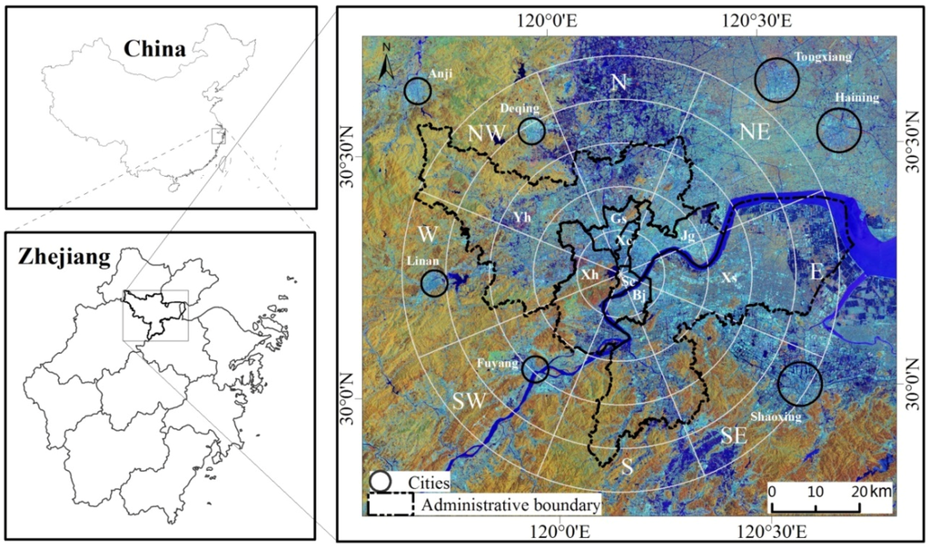
Figure 1.
Study area Hangzhou metropolis, a coastal region in Zhejiang province, China, and the strategy of analyzing impervious surface distribution and its dynamic change with the buffer zone-based approach in different directions. (There are eight administrative units: Yh–Yuhang; Xs–Xiaoshan; Xh–Xihu; Jg–Jianggan; Bj–Binjiang; Gs–Gongshu; Sc–Shangcheng; Xc–Xiacheng. The circles are shown at 10 km intervals for simplification).
Hangzhou metropolis covers eight administrative units—Shangcheng, Xiacheng, Gongsu, Binjiang, Xihu, Jianggan, Yuhang, and Xiaoshan—with a total area of 3068 km2. The administrative boundaries have been modified several times in the past three decades because of rapid urbanization. In the 1980s, the total area of Hangzhou was only 430 km2 with a population of about 5 million. The limitation in land availability made the administration unit expand to 683 km2 in 1996 by incorporating six townships within Xiaoshan and Yuhang counties into Hangzhou. Considering the flat topography on the east side and mountainous regions on the west side, Hangzhou city government proposed the urban expansion policy “urban expansion at the east side and tourism to the west” in 2000 to solve the dilemma of urban expansion space. In March 2001, the administrative area was further expanded from 683 km2 to 3068 km2 by incorporating Xiaoshan and Yuhang counties [51], and a new urban core was established in the southern part of Hangzhou metropolis.
3. Methods
3.1. Data Collection and Preprocessing
Landsat multitemporal imagery with L1T (systematic precision and terrain corrected) products (path/row: 119/39) between 1991 and 2014 was used in this research (Table 1). Six spectral bands with 30 m spatial resolution were used; the thermal band was not used due to its coarse spatial resolution. No image-to-image registration is needed among the multitemporal Landsat images after checking the geometric accuracy among them. In addition, no atmospheric calibration was conducted for these images because we used the individual imagery separately in a hybrid approach for mapping ISA distribution. The ASTER Global Digital Elevation Model (GDEM) data with 30 m spatial resolution was used to examine the impacts of topographic factors on ISA distribution and its dynamic change. The QuickBird images were used for collection of reference data for accuracy assessment of the ISA mapping results. Meanwhile, the boundary file of administrative units was used to analyze the ISA density at the administrative unit scale.

Table 1.
Datasets used in this research.
3.2. Mapping ISA Distribution
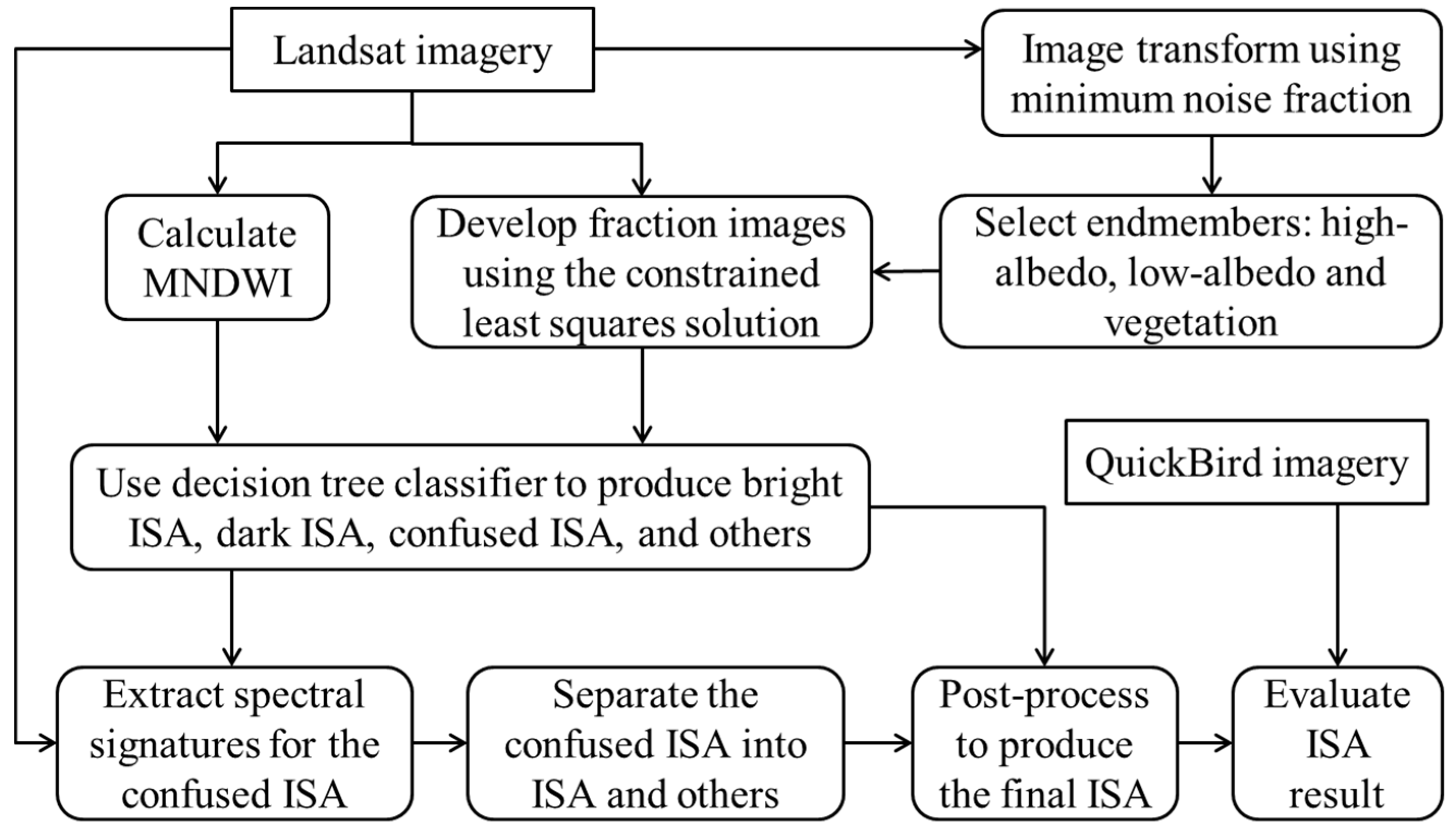
Developing accurate ISA distribution for each date is critical for further examining urban expansion over time. Figure 2 illustrates the hybrid approach to map ISA distribution. The major steps include (1) producing fractional images from Landsat multispectral imagery using the LSMA approach; (2) calculating the modified normalized difference water index (MNDWI) and using it in the decision tree classifier to separate water from other land covers; (3) using the decision tree classifier to produce bright ISA, dark ISA, confused ISA and others based on MNDWI and three fractional images; (4) modifying the confused ISA pixels into ISA and others using cluster analysis (i.e., ISODATA unsupervised classification); and (5) conducting post processing and evaluate the results.

Figure 2.
Framework of mapping impervious surface distribution from Landsat multispectral image. (Note: MNDWI, modified normalized difference water index; ISA, impervious surface area; final ISA is the combination of bright ISA, dark ISA, and other ISA separated from the confusion).
Previous studies have shown that ISA can be accurately extracted from multispectral imagery using the LSMA-based approach [33,34]. One critical step in this approach is to identify representative endmembers. The endmembers can be identified from the scatterplots between spectral bands or transformed components. Previous research has indicated that the transformed components contain the majority of information in the first three components, and the endmembers can be better identified from the components than from spectral bands. Although different transform algorithms such as principal component analysis and minimum noise fraction (MNF) are available, MNF is regarded as an effective approach to extract the majority of information [21,22,34]. In this research, the Landsat multispectral imagery was transformed into a new dataset using MNF. Three endmembers—high-albedo object, low-albedo object, and vegetation—were selected from the scatterplots of the three MNF components [23,41]. A constrained least squares solution was used to unmix the multispectral image into three fraction images and one error image. A detailed description of the LSMA approach can be found in many publications, e.g., [21,52].
Since the high-albedo fraction image contains bright ISA and bare soils, and the low-albedo fraction image contains dark ISA, water/wetland, and shadows, it is critical to remove the non-ISA pixels from the high-albedo and low-albedo fraction images before they are combined to generate an ISA image [33,35]. Because MNDWI is regarded as an effective method to separate water from other land covers [53], this index and the three fraction images were used in a decision tree classifier to extract bright and dark ISA categories [16]. However, some confusion exists among ISA, shallow water, moist soils, and shadows; thus, the multispectral values of these confused classes were retrieved and a cluster analysis (ISODATA) was used to classify the spectral signatures into 30 clusters. The analyst separated them into ISA or others through visual interpretation.
This hybrid approach was used to map ISA distributions separately for the years between 1991 and 2014. In order to further improve ISA mapping performance, the time series ISA distribution data were further examined by checking areas that appeared to have changed between two image dates. For example, generally speaking, if the pixels were ISA in 2010, they should be ISA in 2014; if not, these pixels were visually examined and modified if needed. Sometimes this assumption is not true due to redevelopment of urban areas; that is, the reconstruction of old residential areas might convert urban ISA to grass (a new park).
The final results were evaluated using high spatial resolution QuickBird images from 2010 and 2014. In this research, 300 points were selected using the stratified random sampling technique; that is, the minimum number for ISA was 100 in order to analyze the accuracy of the 2010 and 2014 ISA results. Each point was examined using the QuickBird images, and an error matrix was produced for the ISA images. Overall accuracy (OA), producer accuracy (PA), and user accuracy (UA) were calculated [54]. ISA results in other years were not evaluated due to the lack of reference data, but the accuracies can be assumed similar using this approach [33].
3.3. Spatiotemporal Analysis of ISA Distribution and Its Dynamic Change
3.3.1. Analysis of Spatial Patterns of ISA Distribution and Its Dynamic Change at Pixel Level and Administrative Unit Scale
In order to better understand the ISA distribution patterns, the pixel-based ISA images with a 30 × 30 m cell size were aggregated into fractional ISA images with a cell size of 1 × 1 km; thus, ISA abundance and patterns can be clearly shown through the transition of the fraction values from urban core to rural regions.
Based on time series ISA datasets, the ISA amount and density within administrative units were calculated so we could understand the temporal ISA change at administrative unit scale.
where Di is the ISA density at the ith administrative unit, ISAi is the total ISA area in the ith administrative unit (km2), and Ai is the total area of the ith administrative unit (km2).
Pixel-based change detection is often based on the comparison of classified images at different dates [25]. This research also used the classification-based comparison approach to examine ISA expansion based on the developed ISA images between 1991 and 2014. Average annual ISA change rate (km2/year) was calculated to analyze urbanization rates at temporal scale.
where ISA(t2) and ISA(t1) represent ISA amounts in subsequent (t2) and prior (t1) years, respectively.
3.3.2. Analysis of Spatial Patterns of ISA Distribution and Its Dynamic Change Using the Buffer Zone-Based Approach in Different Directions
The buffer zone-based approach has been used to analyze spatial patterns of land-cover change, including urbanization [20], but previous research mainly analyzed overall spatial patterns within zones without taking different directions into account. Because the spatial patterns of urbanization may be influenced by external factors such as topography, traffic networks, and hydrological networks, it is necessary to examine urban expansion patterns at different aspects. Therefore, we divided this study area into eight directions—east, southeast, south, southwest, west, northwest, north, and northeast—with buffer zones of 2 km intervals within a radius of 50 km (see Figure 1). The objective of using the combination of buffer zones and eight directions is to better understand whether the urban ISA increase is due to infilling within the urban region or expansion into the urban-rural frontier, and where different patterns of urban expansion or infilling occurred in which year or time period. The ISA amounts within the buffer zones in different directions were calculated. Because the buffer zones increase in size as the distances from the urban center increase, it is necessary to remove the impacts of buffer zone size on the ISA amount. The ISA density in a buffer zone is also calculated with Equation (1), but the area is based on each buffer zone. The area for each buffer ring (Aj) is defined as:
where j is the number of each circle, and r is the radius of each circle, from 2, 4, 6, …, to 50 km.
3.4. Impacts of Topography on Urban ISA Distribution and Dynamic Change
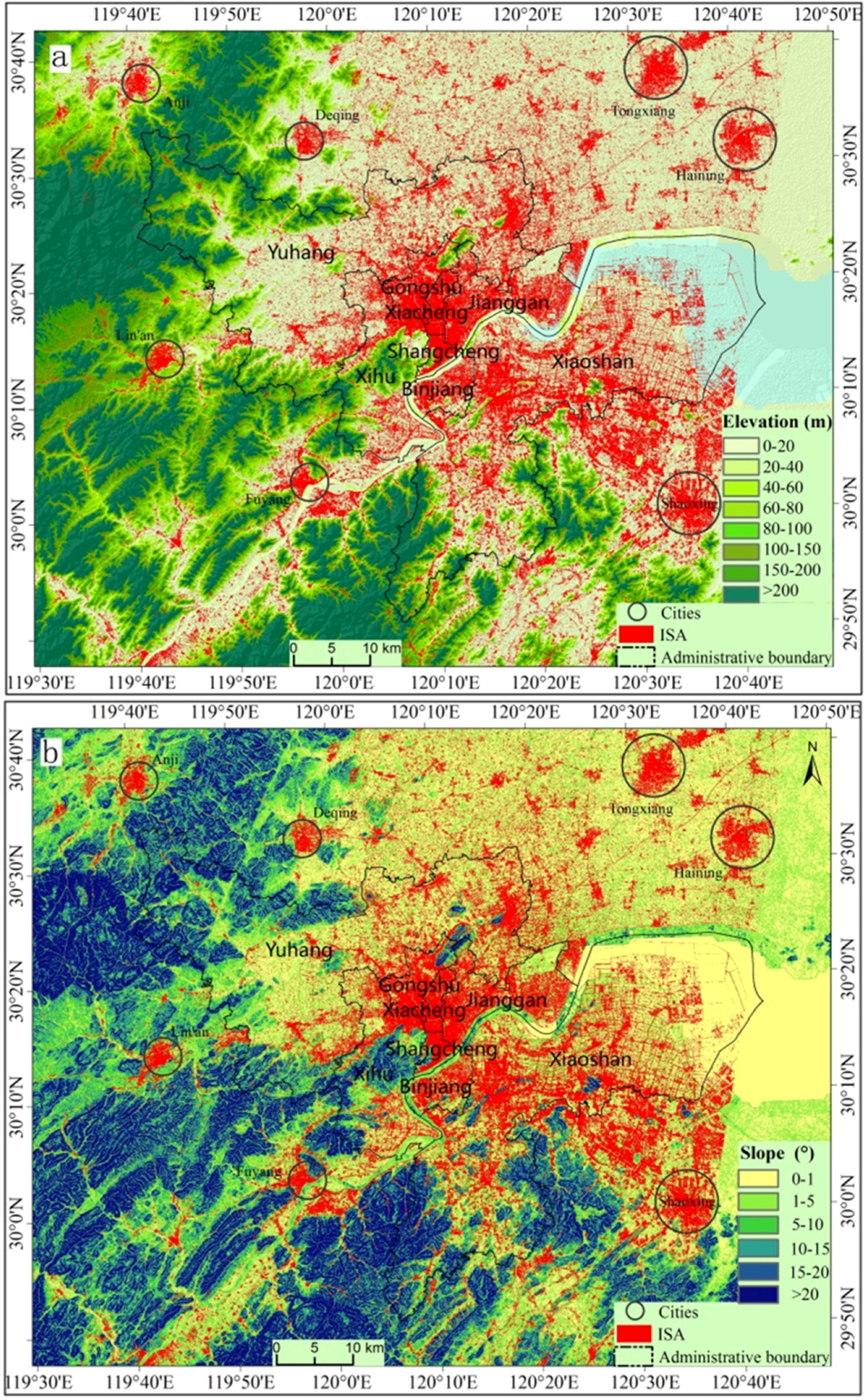
Topography may be an important factor in constraining urban land-cover distribution and its dynamic change, but previous research has not paid much attention to it. In this research, we examined the impacts of elevation and slope on ISA distribution and dynamic change in Hangzhou metropolis. The ASTER GDEM data were used to calculate elevation and slope. Elevation ranges were grouped into six levels: <20, 20–40, 40–60, 60–80, 80–100, and >100 meters; slope ranges were grouped into four levels: <5, 5–10, 10–15, and >15 degrees. The ISA amount for each elevation or slope level was calculated based on ISA data in each given year and grouped elevation or slope images.
4. Results
4.1. Analysis of ISA Distribution and Its Dynamic Change at Pixel Scale
The hybrid approach for mapping ISA distribution produces an OA of over 95% according to the accuracy assessment results for 2010 and 2014 (Table 2). The other dates of ISA results are believed to have similar accuracy using this approach [33], although no accuracy assessment can be conducted because of the difficulty in collecting reference data for historical remote sensing data. These results with high accuracy provide the required data source for further examining the spatial patterns of ISA dynamic change.
Table 2.
Accuracy assessment results of impervious surface area (ISA) mapping of Hangzhou metropolis in 2010 and 2014.
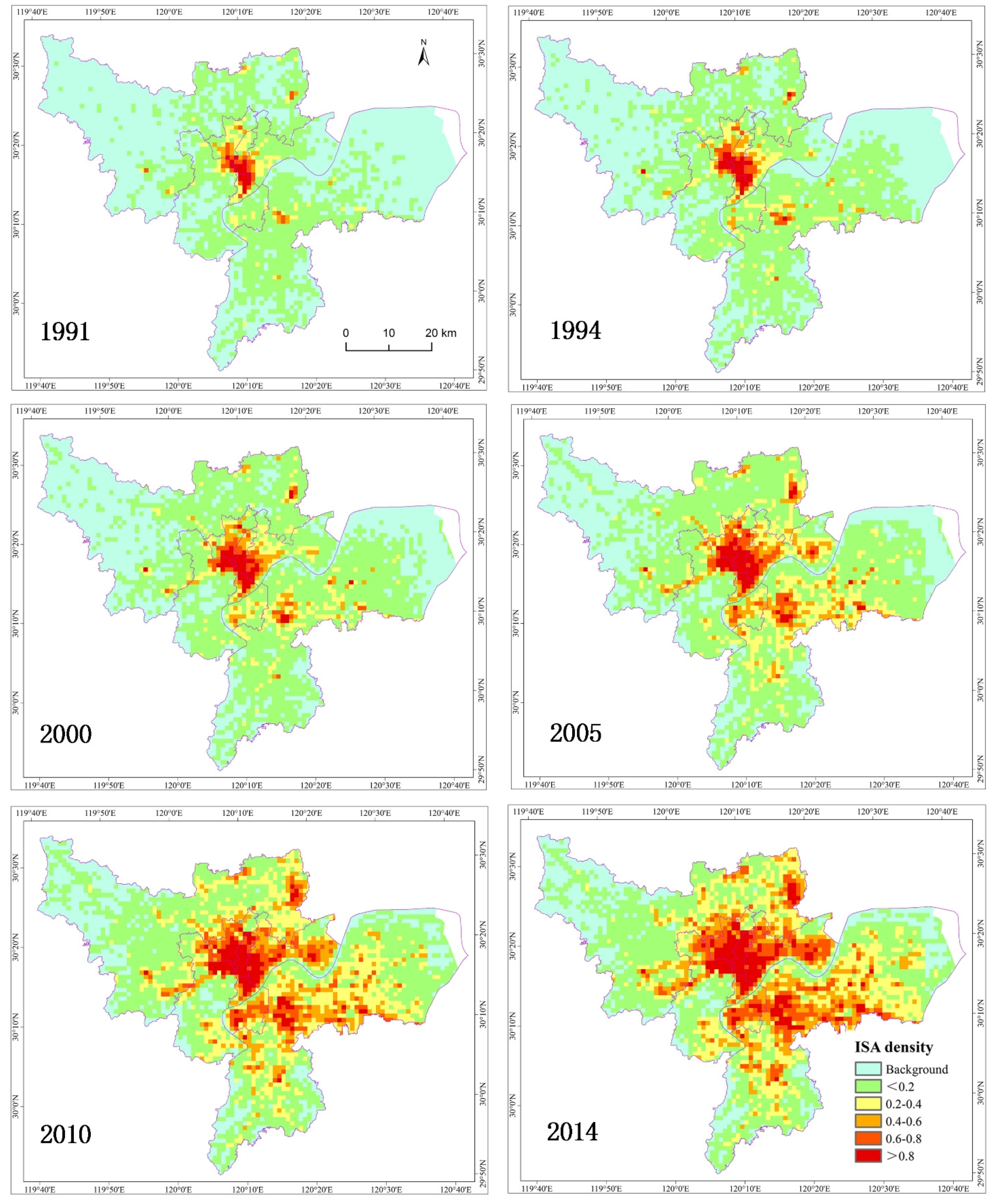
The spatial distributions of ISA density in different years (Figure 3) indicate their different spatial patterns in the past two decades. Overall, the transition of ISA distribution is obvious, from high density in the urban core to low density in rural areas. There was only a single urban core before 2000, but, after 2000, ISA expansion increased rapidly and a new urban core appeared in the southern part—Xiaoshan district. As shown in Figure 4, the ISA expansion was mainly located in the eastern part with flat terrains, due to constraints of mountainous regions in the western part. Before 2000, much ISA increase was in the urban region from infilling open spaces, but in the last 10 years, ISA increase was in the frontiers, especially in the eastern part.

Figure 3.
Comparison of impervious surface area (ISA) density distributions (cell size of 1 km2) at temporal scale showing the ISA transition patterns from urban core to rural regions in Hangzhou metropolis, 1991–2014.
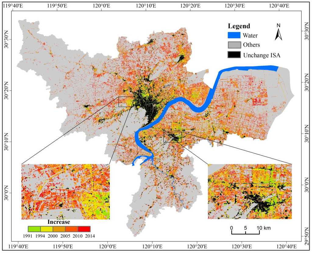
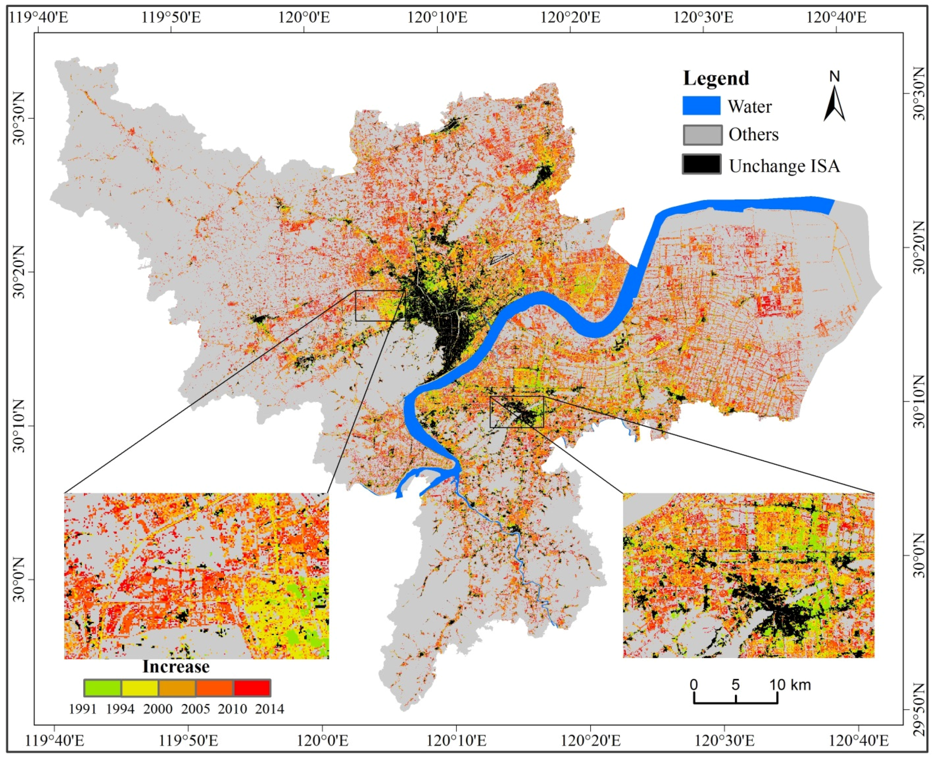
Figure 4.
Dynamic change in impervious surface area (ISA) in Hangzhou metropolis during the change detection periods between 1991 and 2014.
4.2. Analysis of ISA Distribution and Its Dynamic Change at Administrative Units
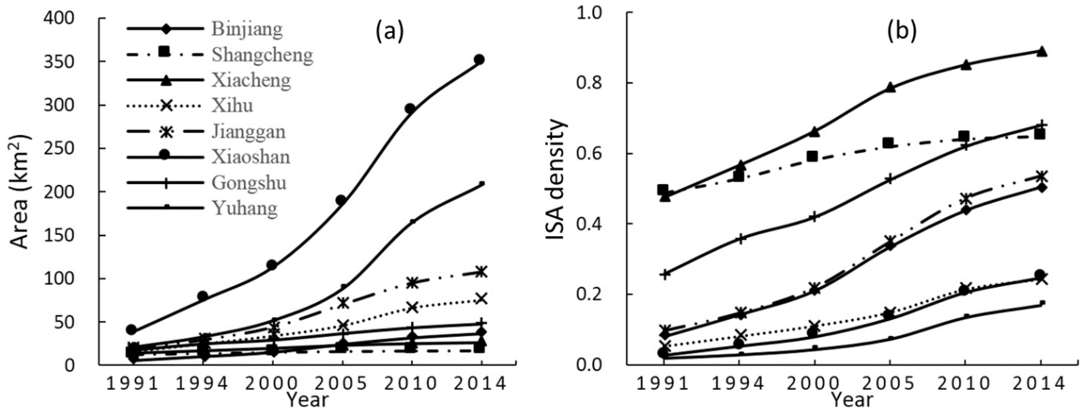
The expansion trends of ISA amounts and densities at administrative units over time (Figure 5) show that Xiaoshan in the southeast and Yuhang in the northwest are the two largest administrative units and have the highest urban expansion areas (see Figure 5a). These two units were merged into Hangzhou metropolis in 2001 because of the constraints of land availability in Hangzhou city. The Xihu district in the southwest and Jianggan district on the east side are two middle size areas and have much smaller ISA amounts than Xiaoshan and Yuhang, but higher than the four small core districts—Binjiang, Shangcheng, Xiacheng, and Gongsu. Xiaoshan and Yuhang have large expanses of land available for urban sprawl, Xihu has limited land available due to West Lake and mountainous areas, and Jianggan has limited land available due to water bodies (river and ocean on the east side). The ISA increases in the four core districts were due to infilling in the urban regions. However, Yuhang and Xiaoshan had the lowest ISA densities in Hangzhou metropolis due to their large agricultural and mountainous areas, while Xihu had low density due to mountains and the lake. It is reasonable that the urban core regions (e.g., Binjiang, Shangcheng, and Gongshu) have higher ISA densities than urban-rural regions (e.g., Yuhang, Xiaoshan) (see Figure 5b). Overall, the ISA density obviously increased for each district from 1991 to 2014.

Figure 5.
Impervious surface area (ISA) amount and density for each administrative unit in Hangzhou metropolis showing the ISA growth over time (Note: (a) represents the trend of ISA amount over time; (b) represents the trend of ISA density over time).
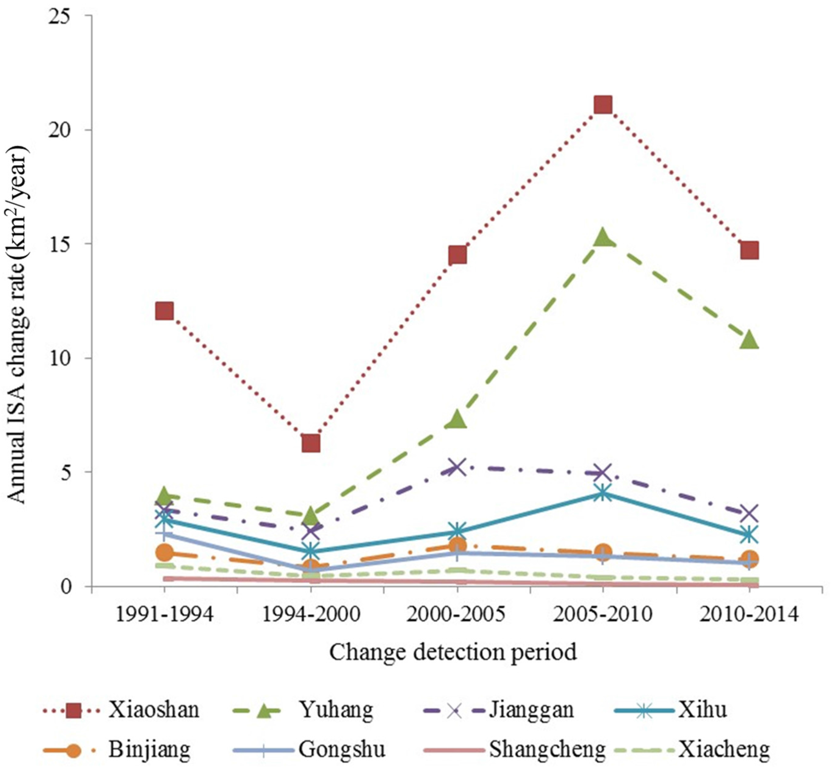
Overall, ISA in Hangzhou metropolis increased rapidly from 146 km2 in 1991 to 868 km2 in 2014 (Table 3). Since entering the 21st century, annual ISA growth rate has been over 33 km2 and as high as 49 km2 in 2005–2010; in contrast, it was only 16 km2 in 1994–2000. There are eight districts in Hangzhou metropolis (see Figure 1). Xiaoshan, located at the east and south sides with flat terrain, has the highest annual ISA growth rate, followed by Yuhang, with flat terrain in the north and northeast and mountains in the west. The core urban regions in Binjiang, Gongshu, Shangcheng, and Xiacheng have very low ISA growth rates (see Figure 6).
Table 3.
Summary of ISA amounts and annual growth rates in Hangzhou metropolis, 1991–2014.
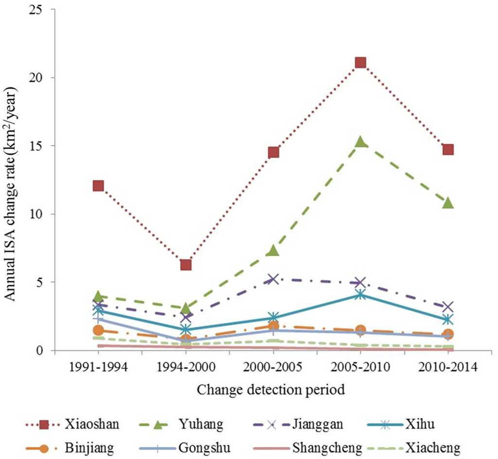
Figure 6.
Comparison of annual growth rates of impervious surface area (ISA) at administrative units of Hangzhou metropolis in different change detection periods.
4.3. Analysis of ISA Distribution at Buffer Zone Scale in Different Directions
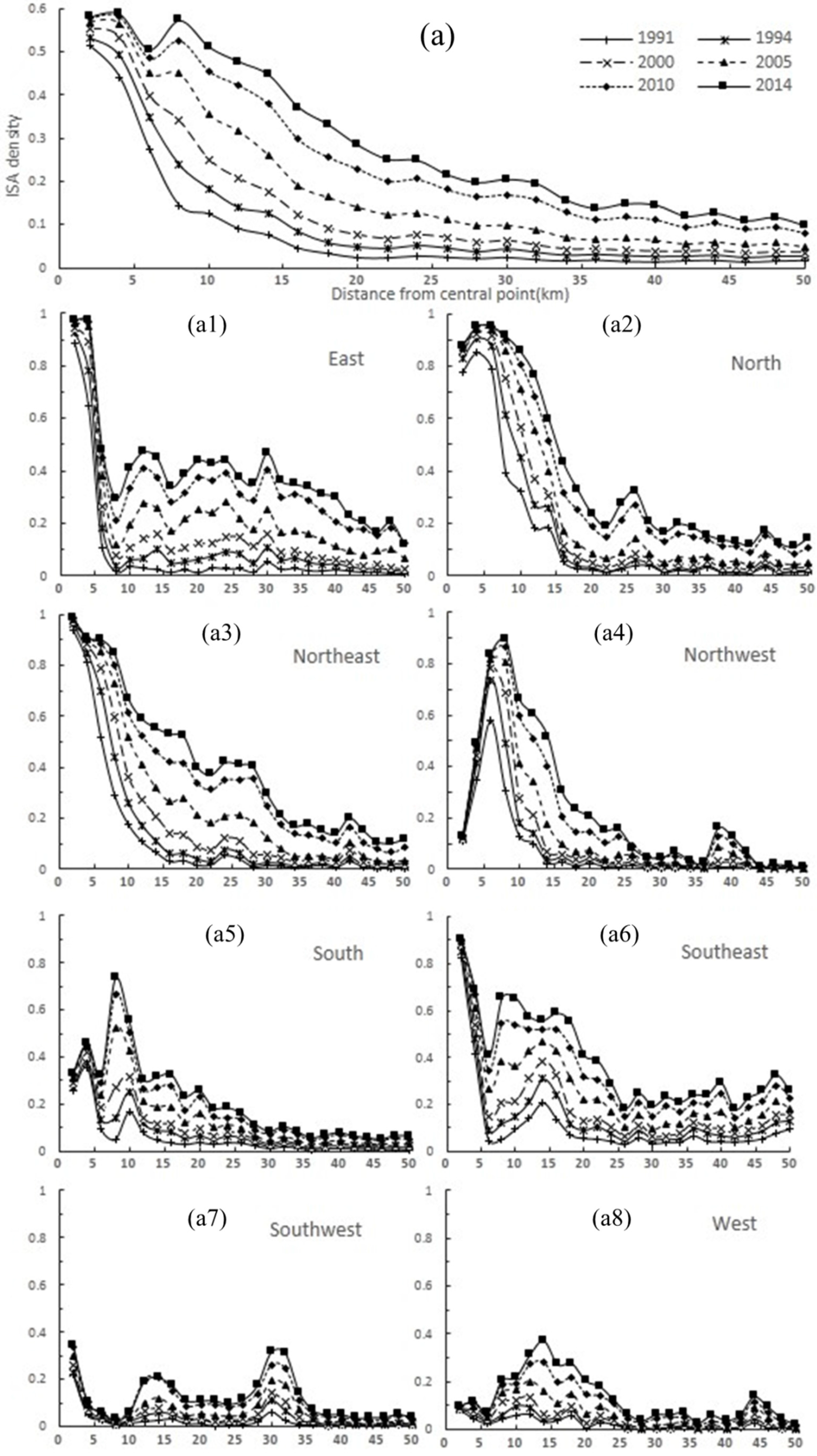
Overall, the ISA distributions had similar trends between 1991 and 2000; that is, ISA density had the highest value within a distance of 4 km from the urban center, decreased gradually until 16 km, and then appeared stable with small density values beyond that distance (see Figure 7a). After 2005, the ISA distribution had a V shape at about 6 km from the urban center, reached a peak around 8 km, and decreased gradually until a distance of around 34 km. Overall, the ISA density for each buffer zone increased. Within a distance of 4 km from the urban center, the density increase value was small, from 0.52 to 0.58 between 1991 and 2014. The highest ISA density increase appeared at distance range of 8–16 km, with increases from 0.12 to 0.58 at around 8 km and 0.05 to 0.37 at 16 km. The ISA density remained stable with low values at 20–50 km between 1991 and 2014 but had the highest increase between 2005 and 2010 for all distance from 6 to 50 km. This result indicates that, before 2000, the major urbanization occurred within a 16 km radius of the urban center, and, after 2000, especially after 2005, urbanization occurred extensively between 6 and 50 km (see Figure 7a).

Figure 7.
Comparison of impervious surface area (ISA) densities at temporal scale in eight directions at 2 km intervals within a radial distance of 50 km from the urban core of Hangzhou metropolis, China (Note: (a) represents the trend of ISA density distribution of entire study area over time; (a1–a8) represent the trend of ISA density distribution at different directions: East—(a1); North—(a2); Northeast—(a3); Northwest—(a4); South—(a5); Southeast—(a6); Southwest—(a7); and West—(a8)).
Analysis of Figure 7a is based on the ISA values of buffer zones at 2 km intervals from the urban center to a distance of 50 km from 1991 to 2014, but this result did not reflect the spatial patterns of ISA density distributions in different directions. Therefore, Figure 7a1–a8 illustrates the ISA density distribution in eight directions in order to understand different spatial patterns of ISA density distribution in various regions.
For east direction with flat terrain (in Figure 7a1), ISA had very high density within the distance of 4 km from the urban center but decreased sharply to the lowest density at 8 km. ISA density was low (less than 0.2) between 8 and 50 km before 2000, but increased considerably to over 0.3 in the distance of 8–40 km in 2014, and the ISA increase was especially fast in this distance range between 2000 and 2010, implying rapid urbanization in the past decade in this direction. In the north direction (Figure 7a2) with flat terrain, ISA density had high values within 6 km, decreased to a valley out to 22 km, and increased gradually to a small peak at 26 km before 2005. ISA density was low from 15 to 50 km, but ISA increased considerably after 2005, especially in the distance of 16 to 50 km between 2005 and 2010, implying that major urbanization occurred in this direction. In the northeast direction (Figure 7a3), high ISA was located within 8 km, decreased gradually to a valley at 22 km, and increased to a small peak at 25 km. Before 2000, ISA was very low between 14 and 50 km. A high ISA increase occurred within 10–32 km between 2000 and 2010, implying rapid urbanization in this region during this period.
In the northwest direction (Figure 7a4), ISA was very low within 6 km but increased sharply to a peak within 6–10 km in 1991–2014. ISA density decreased sharply to its lowest value at 14 km in 1991–2000, and another small peak occurred at 38 km. After 2005, ISA was very low in the distance range of 28–36 km and beyond 44 km due to constraints of mountains in this direction (see Figure 1). In the south direction (Figure 7a5), there were peaks at 4 km and 10 km before 2000, but after that, a higher peak occurred at 8 km. ISA density had small values from 14 to 50 km before 2000. Since 2000, ISA increased at 12–30 km, implying the urbanization occurred in distance range of 6–26 km, especially in 6–12 km, between 2000 and 2010. The mountains limited ISA expansion beyond 30 km. In the southeast (Figure 7a6), very high ISA density appeared within 4 km, decreased sharply to a valley at 6 km, then increased gradually to a peak at 14 km in 1991–2005, and remained at high ISA density from 10 to 24 km in 2010–2014. Because Shaoxing city is located within 42–50 km in this direction, ISA values remained relatively high for the entire distance to 50 km.
Toward the southwest (Figure 7a7) and west (Figure 7a8), ISA density was low because of mountains. In the southwest, there was a peak around 30–32 km due to growth of Fuyang city (see Figure 1), and another small peak at 14 km. In the west direction, a peak occurred at 14 km after 2010. The major southwest urbanization occurred at 12–16 km and 28–34 km in 2005–2010, and the major west urbanization happened between 10 and 24 km in 2010–2014.
This analysis, based on Figure 7a1–a8, indicates different spatial patterns of ISA density in each direction. Major ISA increases were mainly located in the east and northeast directions where there is flat terrain. These different ISA distribution patterns may also be influenced by human-induced factors such as different policies during the years between 1991 and 2014, in addition to constraints of topography.
4.4. Analysis of ISA Dynamic Change at Buffer Zone Scale in Different Directions
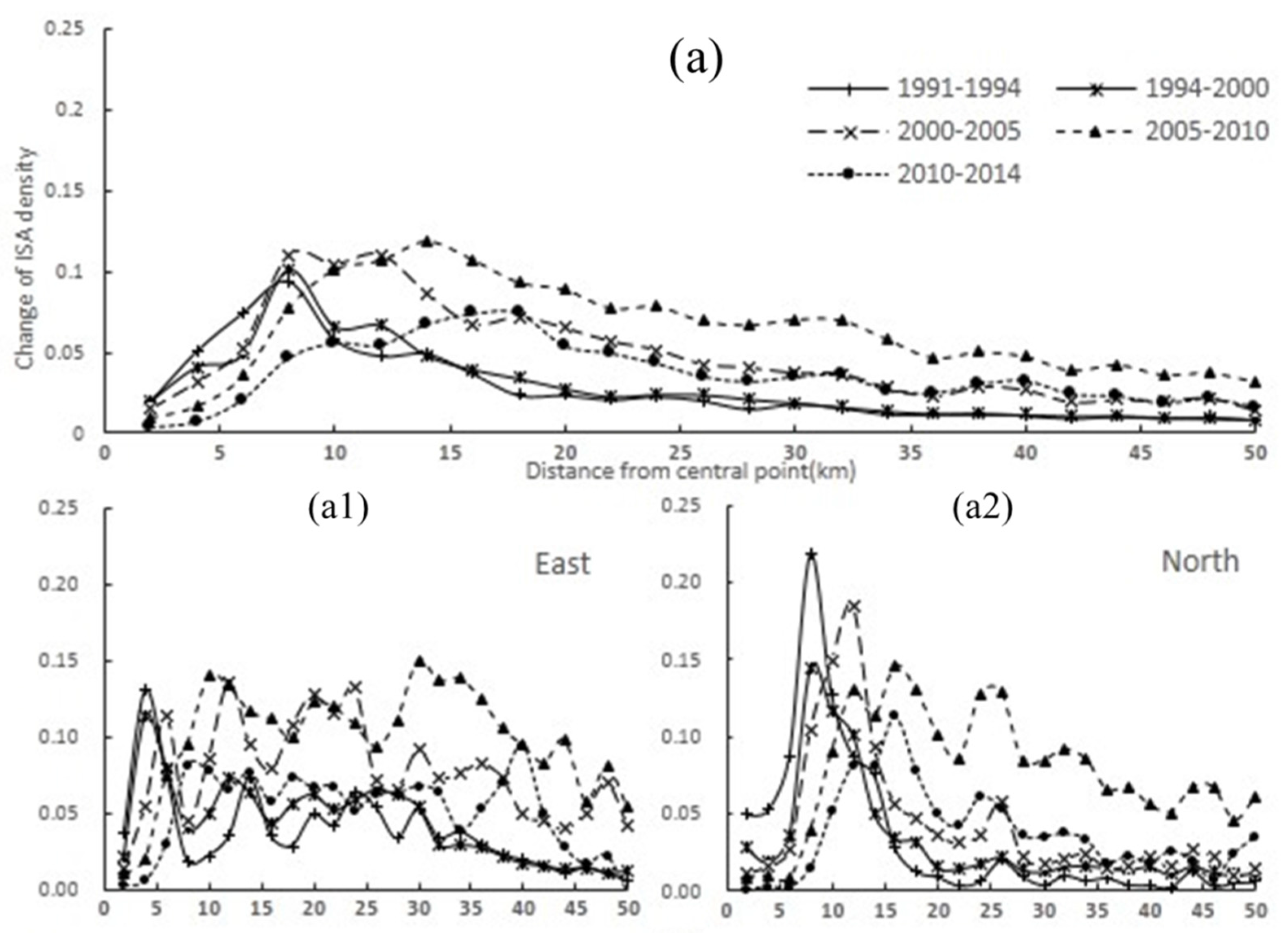
In order to explore the spatial distribution of urban expansion in different directions, Figure 8 provides ISA density change at buffer zones within the change detection periods in eight directions. It indicates that the regions within 8 km from the urban center had higher growth values of ISA density from 1991 to 1994 than in other time periods. The regions within 8–14 km had higher ISA density values from 2000 to 2005, and the regions within 14–50 km had higher values in 2005–2010 (Figure 8a). In 1991–2000, major ISA density growth occurred in the distance range of 4–16 km with the highest at 8 km, implying that major ISA expansion was located in the urban core in this period. In 2000–2005, major ISA density increase occurred between 6 and 26 km, with the highest value in the 8–12 km range; in 2005–2010, the increase was in the distance range of 8–36 km with the highest ISA density growth at 14 km; and in 2010–2014, major ISA density growth occurred within 8–24 km, with the highest at 18 km (see Figure 8a). This indicates that urbanization began in the urban core and shifted gradually to urban-rural frontiers. This result implies that, before 2000, major ISA increase was due to infilling within the urban landscape, and, after 2000, the ISA increase was mainly due to urban expansion into the frontier areas.


Figure 8.
Comparison of impervious surface area (ISA) density change among different change detection periods in eight directions at 2 km intervals within a 50 km radius from Hangzhou metropolis urban center (Note: (a) represents the trend of ISA density change of entire study area over time; (a1–a8) represents the trend of ISA density change at different directions: East—(a1); North—(a2); Northeast—(a3); Northwest—(a4); South—(a5); Southeast—(a6); Southwest—(a7); and West—(a8)).
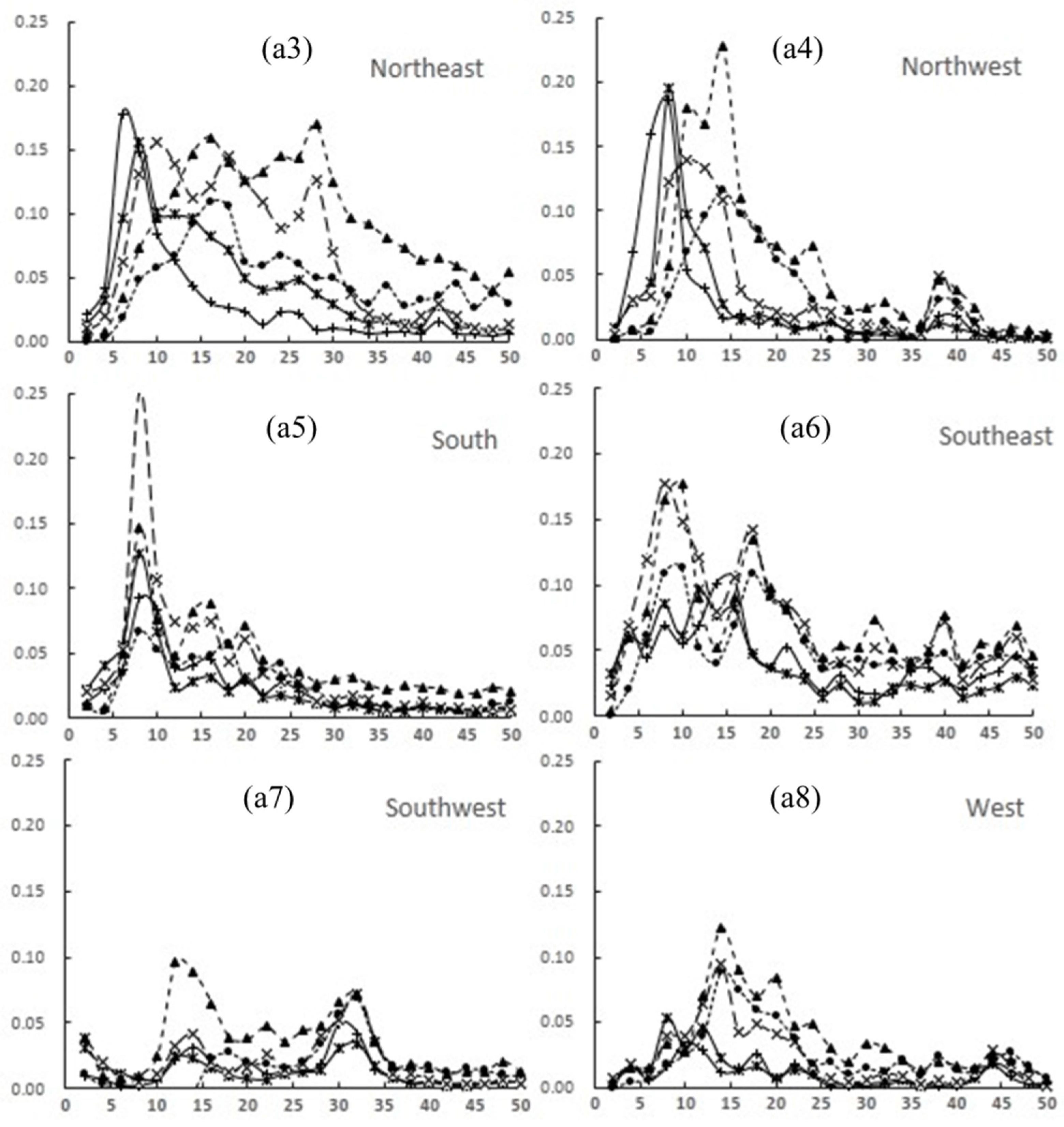
The ISA density change had obviously different spatial patterns in various directions as shown in Figure 8. In the east direction (in Figure 8a1), high ISA density change occurred in the urban core area within 4 km in 1991–2000, the peak shifted to the 20–24 km buffer in 2000–2005, and to the distances of 10–12 km and 30 km in 2000–2010. Overall, the period of 2005–2010 had the highest ISA change, especially from 26 to 50 km in this direction. In the north direction (in Figure 8a2), the peak occurred at 8 km before 2000, and shifted to 12 km in 2000–2005. Within 14–50 km, the highest ISA density value appeared in 2005–2010 compared to the other periods. On the northeast side (in Figure 8a3), the peak was at 6 km before 2000, shifted to 8–10 km in 2000–2005, and to 14–30 km in 2005–2010. In the northwest, the peak was around 8 km before 2005, and shifted to 14 km in 2005–2010. In the south direction, the highest ISA change was located at 8 km for each change detection period, especially in 2000–2005. In the southeast, the highest ISA density changes occurred at basically the same distance, 8–10 km, during the entire study period but especially in 2000–2010. Another high ISA density change was located in 18 km in 2000–2010. In the southwest and west directions, the major ISA increase was at 14 km in 2005–2010. Figure 8 indicates that before 2000, the annual ISA density change was mainly in the east, north, northeast, and northwest directions within a distance range of 5–10 km; with the exception of the northwest, it shifted to 10–30 km in 2000–2005 and farther from the urban center out to 50 km in 2005–2010. In contrast, on the south and west sides, very limited ISA change occurred beyond 25 km. The high ISA changes in the east, northeast, and north were mainly due to flat terrain, and the low ISA changes toward the west and southwest were mainly due to constraints of mountainous terrain.
4.5. Analysis of Topographic Impacts on Urban Expansion
Table 4 summarizes the ISA amount and corresponding percent for different elevation and slope groups for the years between 1991 and 2014. It indicates that majority of ISA amount is distributed in elevation values of less than 20 m, the total ISA amount increased from 211.6 km2 in 1991 to 1400.9 km2 in 2014, and the percent of ISA amount in this group accounting for total ISA amount remain similar, only slight increase from 91.2% in 1991 to 92.3% in 2014. Overall, the ISA amount and percent decreased as elevation increased in the given year. From 1991 to 2014, the ISA amount for each elevation group increased, but the increment became small as elevation increased at the same time period; that is, ISA was expanded in different elevation groups, but the expansion rate became less and less as elevation increased. This implies that urban expansion mainly occurred in the regions with relatively low elevations; and elevation was a constraint factor in urbanization.
Table 4.
Comparison of the relationship of ISA with elevation and slope in Hangzhou metropolis at various time intervals, 1991–2014.
The similar situation is for the slope groups; that is, the majority of ISA amount is located in the areas with slope values of less than 5 degrees, i.e., the area increased from 217.6 km2 in 1991 to 1481.6 km2 in 2014, and the percent increased from 93.8% in 1991 to 97.7% in 2014. As the slope increased, the ISA amount and corresponding percent decreased in the given year. Overall, the ISA amount in each slope group increased from 1991 to 2014, and the increment became less as the slope increased. This means that ISA was expanded from each slope group, but mainly located in the regions with small slopes.
The relationship between ISA amount and elevation or slope groups indicates that the urban expansion is mainly located in the flat terrain areas, and elevation and slope are important constraint factors in urban expansion. This is confirmed in Figure 9, that the majority of ISA is located in the flat regions in north and east sides, but ISA distribution and expansion is constrained by the mountainous regions in west and south sides.

Figure 9.
Impacts of topographic factors—elevation (a) and slope (b) on impervious surface area (ISA) distribution (Note: ISA data were developed from the 2014 Landsat 8 OLI imagery, and elevation and slope are from ASTER GDEM data.)
5. Discussion
5.1. Improvement of ISA Mapping Performance
Urban classification is usually based on training samples using pixel-based classification approaches [55,56], but the confusion between ISA and other land covers (e.g., bare soils, water/wetland) often results in poor classification accuracy for detailed urban land-cover classification [16,18,34,56]. The relatively coarse spatial resolution images (e.g., the common remote sensing data of Landsat imagery) worsen the detailed urban land-cover classification due to mixed pixel problem and complex urban land-cover composition [18,31,57]. Previous research has proven the LSMA-based approach can effectively extract ISA [16,22,33,58], and we further modified the previous approach and produced ISA distribution with overall accuracy of 95% using a hybrid approach consisting of LSMA, vegetation index, decision tree classifier, and cluster analysis. This research indicated that the hybrid approach is effective for producing accurate ISA distribution, which is especially necessary for examining urban expansion [33,34]. One critical step is to solve the confusion between some ISA pixels and other land covers such as bare soils and wetlands that have spectral signatures similar to bright and dark ISAs. This research used MNDWI to separate dark ISA and water/wetland and the analyst’s knowledge to further separate the ISA from other land covers in the confused class. This research indicated that complete separation of ISA from other land covers is still very difficult and a human expert is needed to further separate them in the post-processing stage.
Analysis of land-cover spatial distribution is often based on pixel-based results [59] but might not show the spatial patterns of a land cover [17]. This research aggregated the ISA results from the pixel level at a cell size of 30 × 30 m to fractional values at a cell size of 1 × 1 km to show clearly the ISA transition from the urban core to rural areas. This implies the necessity of developing fractional ISA distribution, especially when medium or coarse spatial resolution images are used for ISA mapping [17,36,60]. The availability of very high spatial resolution images such as QuickBird, Pleiades, and Worldview with half-meter spatial resolution provides a new platform for accurately producing ISA data, which can be used to calibrate the medium or coarse spatial resolution images [36,60].
5.2. Examination of ISA Expansion and Roles of the Buffer Zone–Based Approach
Previous research only examined overall land-cover change without exploring the detailed change of spatial patterns in different directions from the urban core [20]. This research not only provided the overall ISA change at pixel scale, but also examined the ISA spatial patterns in eight directions and at distances using the buffer zone–based approach. This kind of analysis provided much rich information about ISA spatial pattern change and is valuable for explaining why different geographic locations have different urbanization patterns and rates. Through the analysis of ISA density distribution and its dynamic change using buffer zones in different directions between 1991 and 2014, we can better understand the urbanization characteristics; that is, the ISA increase in urban core is mainly due to the infilling of open space or redevelopment of old urban landscapes, and the ISA increase in urban-rural frontier is mainly due to the urban expansion through the conversion of agriculture lands to built-up areas. Through this research, we can better understand the history of urbanization from urban regions to rural areas with different stages having their own urbanization patterns and rates. This kind of data source or information is especially useful for understanding the effects of previously implemented policies on urbanization patterns and paces.
Previous research has indicated that rapid increase of ISA can aggravate the pollution density in a lake or river [61], and the results in this research will be useful to examine the impacts of urbanization on water quality in West Lake, which is a famous tourism site in Hangzhou. In addition, urbanization can result in UHI, and spatial patterns of different ISA expansion directions can intensify the UHIs in those directions [9,10,47,62,63]. Therefore, the spatial patterns of ISA expansion in this research will be valuable for use in examining UHI spatial patterns in Hangzhou metropolis. The buffer zone approach in different directions may provide new insights for examining the relationships between urbanization and UHI, and more research is needed in the future.
5.3. Effects of Topographic Factors and Policies on Urban Expansion Patterns
China’s overall ISA growth rate was faster before 2000 compared to later [64], but Hangzhou metropolis had a higher ISA growth rate after 2000 compared to before. This is because the city’s urban traffic network construction project promoted ISA expansion into the urban-rural frontiers. After 2010, the metropolis had a development strategy that enhanced the optimization of inner city function and structure and improved intensive use of its land, resulting in a relatively lower ISA expansion rate in 2010–2014 than in 2005–2010. This implies the important role of policies in urban expansion; that is, a new policy may considerably promote urban expansion speed in the short term. This kind of policy may result in improved economic conditions; thus, good economic condition is often an important factor in fast urban expansion [65].
Population and economic conditions are often regarded as the major factors influencing urbanization patterns and rates [20,57]. However, these factors may not directly influence urban expansion; instead, other factors such as policies, topography, hydrology, and land availability are important but are difficult to quantify [57] when examining their relationships with urbanization rates and spatial patterns. At the same time, urban expansion does not simply occur in a single city. It is often influenced by neighboring cities, especially satellite cities surrounding a big city, as in Hangzhou metropolis (see Figure 1). More research is needed to examine the different roles of external factors on urbanization in order to provide scientific foundations for better urban planning and management.
6. Conclusions
This research selected Hangzhou metropolis as a case study to examine spatial patterns of ISA distribution and its dynamic change in administrative units and radial buffer zones in different directions using multitemporal Landsat imagery between 1991 and 2014. The following conclusions can be obtained from this research:
- (1)
- The hybrid approach can effectively extract ISA distribution with an overall accuracy of over 95%, and both producer and user accuracies of over 91%. This approach provided the fundamental data sources for examining urban dynamic change over time.
- (2)
- ISA in Hangzhou metropolis increased from 146 km2 in 1991 to 868 km2 in 2014. Annual ISA growth rates were between 15.6 km2/year and 48.8 km2/year with the lowest growth rate in 1994–2000 and the highest growth rate in 2005–2010.
- (3)
- Urban expansion has various rates and patterns at different distances from the urban center in various directions between 1991 and 2014. Topographic factors, especially slope, are important constraints influencing spatial patterns of urban distribution and expansion.
- (4)
- Policies may be important factors influencing urbanization patterns and rates, but they are difficult to quantify.
Acknowledgments
This study was financially supported by Zhejiang A & F University’s Research and Development Fund for the talent startup project (2013FR052).
Author Contributions
Longwei Li conducted data collection and processing. Dengsheng Lu designed the research procedure, conducted result analysis, and wrote the manuscript. Wenhui Kuang joined preparation of the manuscript.
Conflicts of Interest
The authors declare no conflicts of interest.
References
- Yin, J.; Yin, Z.; Zhong, H.; Xu, S.; Hu, X.; Wang, J.; Wu, J. Monitoring urban expansion and land use/land cover changes of Shanghai metropolitan area during the transitional economy (1979–2009) in China. Environ. Monit. Assess. 2011, 177, 609–621. [Google Scholar] [CrossRef] [PubMed]
- Liu, Z.; He, C.; Zhang, Q.; Huang, Q.; Yang, Y. Extracting the dynamics of urban expansion in China using DMSP-OLS nighttime light data from 1992 to 2008. Landsc. Urban Plan. 2012, 106, 62–72. [Google Scholar] [CrossRef]
- Schneider, A. Monitoring land cover change in urban and peri-urban areas using dense time stacks of Landsat satellite data and a data mining approach. Remote Sens. Environ. 2012, 124, 689–704. [Google Scholar] [CrossRef]
- Wang, L.; Li, C.; Ying, Q.; Cheng, X.; Wang, X.; Li, X.; Hu, L.; Liang, L.; Yu, L.; Huang, H.; et al. China’s urban expansion from 1990 to 2010 determined with satellite remote sensing. Chin. Sci. Bull. 2012, 57, 2802–2812. [Google Scholar] [CrossRef]
- Schneider, A.; Chang, C.; Paulsen, K. The changing spatial form of cities in Western China. Landsc. Urban Plan. 2015, 135, 40–61. [Google Scholar] [CrossRef]
- He, C.; Liu, Z.; Tian, J.; Ma, Q. Urban expansion dynamics and natural habitat loss in China: A multiscale landscape perspective. Glob. Chang. Biol. 2014, 20, 2886–2902. [Google Scholar] [CrossRef] [PubMed]
- Srinivasan, V.; Seto, K.C.; Emerson, R.; Gorelick, S.M. The impact of urbanization on water vulnerability: A coupled human–environment system approach for Chennai, India. Glob. Environ. Chang. 2013, 23, 229–239. [Google Scholar] [CrossRef]
- Schneider, A.; Mertes, C.M. Expansion and growth in Chinese cities, 1978–2010. Environ. Res. Lett. 2014, 9. [Google Scholar] [CrossRef]
- Yuan, F.; Bauer, M.E. Comparison of impervious surface area and normalized difference vegetation index as indicators of surface urban heat island effects in Landsat imagery. Remote Sens. Environ. 2007, 106, 375–386. [Google Scholar] [CrossRef]
- Myint, S.W.; Zheng, B.; Talen, E.; Fan, C.; Kaplan, S.; Middel, A.; Smith, M.; Huang, H.; Brazel, A. Does the spatial arrangement of urban landscape matter? Examples of urban warming and cooling in Phoenix and Las Vegas. Ecosyst. Health Sustain. 2015, 1. [Google Scholar] [CrossRef]
- Xu, H.; Lin, D.; Tang, F. The impact of impervious surface development on land surface temperature in a subtropical city: Xiamen, China. Int. J. Climatol. 2013, 33, 1873–1883. [Google Scholar] [CrossRef]
- Xian, G. Satellite remotely-sensed land surface parameters and their climatic effects for three metropolitan regions. Adv. Space Res. 2008, 41, 1861–1869. [Google Scholar] [CrossRef]
- Wu, J.; He, C.; Huang, G.; Yu, D. Urban Landscape Ecology: Past, Present, and Future. In Landscape Ecology for Sustainable Environment and Culture; Fu, B., Jones, K.B., Eds.; Springer Science & Business Media: Dordrecht, The Netherlands, 2013; Chapter 3; pp. 37–53. [Google Scholar]
- Fan, P.; Xie, Y.; Qi, J.; Chen, J.; Huang, H. Vulnerability of a coupled natural and human system in a changing environment: Dynamics of Lanzhou’s urban landscape. Landsc. Ecol. 2014, 29, 1709–1723. [Google Scholar] [CrossRef]
- Michishita, R.; Jiang, Z.; Xu, B. Monitoring two decades of urbanization in the Poyang Lake area, China through spectral unmixing. Remote Sens. Environ. 2012, 117, 3–18. [Google Scholar] [CrossRef]
- Zhang, C.; Chen, Y.; Lu, D. Mapping the land-cover distribution in arid and semiarid urban landscapes with Landsat Thematic Mapper imagery. Int. J. Remote Sens. 2015, 36, 4483–4500. [Google Scholar] [CrossRef]
- Zhang, C.; Chen, Y.; Lu, D. Detecting fractional land-cover change in arid and semiarid urban landscapes with multitemporal Landsat Thematic Mapper imagery. GISci. Remote Sens. 2015, 52, 700–722. [Google Scholar] [CrossRef]
- Myint, S.W.; Gober, P.; Brazel, A.; Grossman-Clarke, S.; Weng, Q. Per-pixel versus object-based classification of urban land cover extraction using high spatial resolution imagery. Remote Sens. Environ. 2011, 115, 1145–1161. [Google Scholar] [CrossRef]
- Sexton, J.O.; Song, X.; Huang, C.; Channan, S.; Baker, M.E.; Townshend, J.R. Urban growth of the Washington, D.C.–Baltimore, MD metropolitan region from 1984 to 2010 by annual Landsat-based estimates of impervious cover. Remote Sens. Environ. 2013, 129, 42–53. [Google Scholar] [CrossRef]
- Kuang, W.; Chi, W.; Lu, D.; Dou, Y. A comparative analysis of megacity expansions in China and the U.S.: Patterns, rates and driving forces. Landsc. Urban Plan. 2014, 132, 121–135. [Google Scholar] [CrossRef]
- Lu, D.; Weng, Q. Use of Impervious Surface in Urban Land Use Classification. Remote Sens. Environ. 2006, 102, 146–160. [Google Scholar] [CrossRef]
- Wu, C.; Murray, A.T. Estimating impervious surface distribution by spectral mixture analysis. Remote Sens. Environ. 2003, 84, 493–505. [Google Scholar] [CrossRef]
- Li, X.; Gong, P.; Liang, L. A 30-year (1984–2013) record of annual urban dynamics of Beijing City derived from Landsat data. Remote Sens. Environ. 2015, 166, 78–90. [Google Scholar] [CrossRef]
- Powell, S.; Cohen, W.B.; Yang, Z.; Pierce, J.D.; Alberti, M. Quantification of impervious surface in the Snohomish Water Resources Inventory Area of Western Washington from 1972 to 2006. Remote Sens. Environ. 2008, 112, 1895–1908. [Google Scholar] [CrossRef]
- Lu, D.; Li, G.; Moran, E. Current situation and needs of change detection techniques. Int. J. Image Data Fusion 2014, 5, 13–38. [Google Scholar] [CrossRef]
- Lu, D.; Mausel, P.; Brondízio, E.; Moran, E. Change Detection Techniques. Int. J. Remote Sens. 2004, 25, 2365–2407. [Google Scholar] [CrossRef]
- Bhagat, V.S. Use of remote sensing techniques for robust digital change detection of land: A review. Recent Pat. Space Technol. 2012, 2, 123–144. [Google Scholar] [CrossRef]
- Coppin, P.; Jonckheere, I.; Nackaerts, K.; Muys, B.; Lambin, E. Digital change detection methods in ecosystem monitoring: A review. Int. J. Remote Sens. 2004, 25, 1565–1596. [Google Scholar] [CrossRef]
- Hansen, M.C.; Loveland, T.R. A review of large area monitoring of land cover change using Landsat data. Remote Sens. Environ. 2012, 122, 66–74. [Google Scholar] [CrossRef]
- Im, J.; Jensen, J.R.; Tullis, J.A. Object-based change detection using correlation image analysis and image segmentation. Int. J. Remote Sens. 2008, 29, 399–423. [Google Scholar] [CrossRef]
- Lu, D.; Weng, Q. Spectral Mixture Analysis of the Urban Landscapes in Indianapolis with Landsat ETM+ Imagery. Photogramm. Eng. Remote Sens. 2004, 70, 1053–1062. [Google Scholar] [CrossRef]
- Weng, Q. Remote sensing of impervious surfaces in the urban areas: Requirements, methods, and trends. Remote Sens. Environ. 2012, 117, 34–49. [Google Scholar] [CrossRef]
- Lu, D.; Moran, E.; Hetrick, S. Detection of Impervious Surface Change with Multitemporal Landsat Images in an Urban-rural Frontier. ISPRS J. Photogramm. Remote Sens. 2011, 66, 298–306. [Google Scholar] [CrossRef] [PubMed]
- Lu, D.; Li, G.; Kuang, W.; Moran, E. Methods to extract impervious surface areas from satellite images. Int. J. Digit. Earth 2014, 7, 93–112. [Google Scholar] [CrossRef]
- Weng, Q. Remote Sensing of Impervious Surfaces; CRC Press: Boca Raton, FL, USA, 2007; p. 488. [Google Scholar]
- Guo, W.; Lu, D.; Wu, Y.; Zhang, J. Mapping impervious surface distribution with integration of SNNP VIIRS-DNB and MODIS NDVI data. Remote Sens. 2015, 7, 12459–12477. [Google Scholar] [CrossRef]
- Zhang, H.; Lin, H.; Zhang, Y.; Weng, Q. Remote Sensing of Impervious Surfaces in Tropical and Subtropical Areas; CRC Press: Boca Raton, FL, USA, 2015; p. 174. [Google Scholar]
- Xian, G.; Homer, C. Updating the 2001 National Land Cover Database Impervious Surface Products to 2006 using Landsat Imagery Change Detection Methods. Remote Sens. Environ. 2010, 114, 1676–1686. [Google Scholar] [CrossRef]
- Mountrakis, G.; Li, L. Enhancing and replacing spectral information with intermediate structural inputs: A case study on impervious surface detection. Remote Sens. Environ. 2011, 115, 1162–1170. [Google Scholar] [CrossRef]
- Yang, F.; Matsushita, B.; Fukushima, T.; Yang, W. Temporal mixture analysis for estimating impervious surface area from multi-temporal MODIS NDVI data in Japan. ISPRS J. Photogramm. Remote Sens. 2012, 72, 90–98. [Google Scholar] [CrossRef]
- Weng, Q.; Lu, D.; Schubring, J. Estimation of land surface temperature–vegetation abundance relationship for urban heat island studies. Remote Sens. Environ. 2004, 89, 467–483. [Google Scholar] [CrossRef]
- Bauer, M.E.; Loffelholz, B.C.; Wilson, B. Estimating and mapping impervious surface area by regression analysis of Landsat imagery. In Remote Sensing of Impervious Surfaces; Weng, Q., Ed.; CRC Press: Boca Raton, FL, USA, 2008; pp. 3–19. [Google Scholar]
- Kaspersen, P.S.; Fensholt, R.; Drews, M. Using Landsat Vegetation Indices to Estimate Impervious Surface Fractions for European Cities. Remote Sens. 2015, 7, 8224–8249. [Google Scholar] [CrossRef]
- Ridd, M.K. Exploring a V-I-S (vegetation-impervious surface-soil) model for urban ecosystem analysis through remote sensing: Comparative anatomy for cities. Int. J. Remote Sens. 1995, 16, 2165–2185. [Google Scholar] [CrossRef]
- Weng, Q.; Liu, H.; Lu, D. Assessing the Effects of Land Use and Land Cover Patterns on Thermal Conditions Using Landscape Metrics in City of Indianapolis, United States. Urban Ecosyst. 2007, 10, 203–219. [Google Scholar] [CrossRef]
- Weng, Q.; Lu, D. A Sub-pixel Analysis of Urbanization Effect on Land Surface Temperature and its Interplay with Impervious Surface and Vegetation Coverage in Indianapolis, United States. Int. J. Appl. Earth Obs. Geoinf. 2008, 10, 68–83. [Google Scholar] [CrossRef]
- Fan, C.; Myint, S.W.; Zheng, B. Measuring the spatial arrangement of urban vegetation and its impacts on seasonal surface temperatures. Prog. Phys. Geogr. 2015, 39, 199–219. [Google Scholar] [CrossRef]
- Lu, D.; Hetrick, S.; Moran, E.; Li, G. Detection of urban expansion in an urban-rural landscape with multitemporal QuickBird images. J. Appl. Remote Sens. 2010, 4. [Google Scholar] [CrossRef] [PubMed]
- Hangzhou City Climate Characteristics. Available online: http://www.hangzhou.gov.cn/main/zjhz/hzlj/2007/zsh/T232609.shtml (accessed on 20 May 2015).
- Zhejiang Statistical Bureau. Zhejiang Statistical Yearbook; China Statistics Press: Beijing, China, 2014. (In Chinese)
- Hangzhou City Administrative Division Adjustment. Available online: http://www.people.com.cn/GB/shizheng/19/20010312/415229.html (accessed on 20 May 2015).
- Mustard, J.F.; Sunshine, J.M. Spectral analysis for earth science: Investigations using remote sensing data. Remote Sens. Earth Sci. Man. Remote Sens. 1999, 3, 251–307. [Google Scholar]
- Xu, H. A study on information extraction of water body with the modified normalized difference water index (MNDWI). J. Remote Sens. 2005, 5, 589–595. [Google Scholar]
- Congalton, R.G.; Green, K. Assessing the Accuracy of Remotely Sensed Data: Principles and Practices, 2nd ed.; CRC Press: Boca Raton, FL, USA, 2008. [Google Scholar]
- Lu, D.; Weng, Q. A Survey of Image Classification Methods and Techniques for Improving Classification Performance. Int. J. Remote Sens. 2007, 28, 823–870. [Google Scholar] [CrossRef]
- Lu, D.; Weng, Q. Urban Classification Using Full Spectral Information of Landsat ETM+ Imagery in Marion County, Indiana. Photogramm. Eng. Remote Sens. 2005, 71, 1275–1284. [Google Scholar] [CrossRef]
- Kuang, W.; Liu, J.; Dong, J.; Chi, W.; Zhang, C. The rapid and massive urban and industrial land expansions in China between 1990 and 2010: A CLUD-based analysis of their trajectories, patterns, and drivers. Landsc. Urban Plan. 2016, 145, 21–33. [Google Scholar] [CrossRef]
- Deng, C.; Wu, C. A spatially adaptive spectral mixture analysis for mapping subpixel urban impervious surface distribution. Remote Sens. Environ. 2013, 133, 62–70. [Google Scholar] [CrossRef]
- Lu, D.; Li, G.; Moran, E.; Hetrick, S. Spatiotemporal analysis of land-use and land-cover change in the Brazilian Amazon. Int. J. Remote Sens. 2013, 34, 5953–5978. [Google Scholar] [CrossRef] [PubMed]
- Lu, D.; Tian, H.; Zhou, G.; Ge, H. Regional Mapping of Human Settlements in Southeastern China with Multisensor Remotely Sensed Data. Remote Sens. Environ. 2008, 112, 3668–3679. [Google Scholar] [CrossRef]
- Kuang, W. Evaluating impervious surface growth and its impacts on water environment in Beijing-Tianjin-Tangshan Metropolitan Area. J. Geogr. Sci. 2012, 22, 535–547. [Google Scholar] [CrossRef]
- Kuang, W.; Dou, Y.; Zhang, C.; Chi, W.; Liu, A.; Liu, Y.; Zhang, R.; Liu, J. Quantifying the heat flux regulation of metropolitan land-use/land-cover components by coupling remote sensing-modelling with in situ measurement. J. Geogr. Res. Atmos. 2015, 120, 113–130. [Google Scholar] [CrossRef]
- Kuang, W.; Liu, Y.; Dou, Y.; Chi, W.; Chen, G.; Gao, C.; Yang, T.; Liu, J.; Zhang, R. What are hot and what are not in an urban landscape: Quantifying and explaining the land surface temperature pattern in Beijing, China. Landsc. Ecol. 2015, 30, 357–373. [Google Scholar] [CrossRef]
- Kuang, W.; Liu, J.; Zhang, Z.; Lu, D.; Xiang, B. Spatiotemporal dynamics of impervious surface areas across China during the early 21st century. Chin. Sci. Bull. 2013, 58, 1691–1701. [Google Scholar] [CrossRef]
- Lu, D.; Xu, X.; Tian, H.; Moran, E.; Zhao, M.; Running, S. The effects of urbanization on net primary productivity in Southeastern China. Environ. Manag. 2010, 46, 404–410. [Google Scholar] [CrossRef] [PubMed]
© 2016 by the authors; licensee MDPI, Basel, Switzerland. This article is an open access article distributed under the terms and conditions of the Creative Commons by Attribution (CC-BY) license (http://creativecommons.org/licenses/by/4.0/).