Article

Novel Approach to Unsupervised Change Detection Based on a Robust Semi-Supervised FCM Clustering Algorithm

1
School of Remote Sensing and Information Engineering, Wuhan University, No. 129 of Luoyu Road, Wuhan 430079, China
2
Joint Spatial Information Research Laboratory of Wuhan University and Hong Kong Polytechnic University, Wuhan University, No. 129 of Luoyu Road, Wuhan 430079, China
3
School of Environment Science and Spatial Informatics, China University of Mining and Technology, Xuzhou 221116, China
*
Author to whom correspondence should be addressed.
Remote Sens. 2016, 8(3), 264; https://doi.org/10.3390/rs8030264
Submission received: 20 November 2015 / Revised: 20 January 2016 / Accepted: 11 March 2016 / Published: 22 March 2016

Abstract

:
This study presents a novel approach for unsupervised change detection in multitemporal remotely sensed images. This method addresses the problem of the analysis of the difference image by proposing a novel and robust semi-supervised fuzzy C-means (RSFCM) clustering algorithm. The advantage of the RSFCM is to further introduce the pseudolabels from the difference image compared with the existing change detection methods; these methods, mainly use difference intensity levels and spatial context. First, the patterns with a high probability of belonging to the changed or unchanged class are identified by selectively thresholding the difference image histogram. Second, the pseudolabels of these nearly certain pixel-patterns are jointly exploited with the intensity levels and spatial information in the properly defined RSFCM classifier in order to discriminate the changed pixels from the unchanged pixels. Specifically, labeling knowledge is used to guide the RSFCM clustering process to enhance the change information and obtain a more accurate membership; information on spatial context helps to lower the effect of noise and outliers by modifying the membership. RSFCM can detect more changes and provide noise immunity by the synergistic exploitation of pseudolabels and spatial context. The two main contributions of this study are as follows: (1) it proposes the idea of combining the three information types from the difference image, namely, (a) intensity levels, (b) labels, and (c) spatial context; and (2) it develops the novel RSFCM algorithm for image segmentation and forms the proposed change detection framework. The proposed method is effective and efficient for change detection as confirmed by six experimental results of this study.

Graphical Abstract

1. Introduction

Remote sensing data change detection is the process of identifying land cover changes using remotely sensed imagery of the same scene acquired at different times [1,2]. In past decades, numerous change detection methods were developed, and many have been summarized and reviewed [1,2,3,4,5,6]. The methods can be broadly categorized into either supervised or unsupervised based on the nature of their data processing.
This study focuses on one of the most widely used types of unsupervised change detection methods based on the difference image. From a methodological perspective, difference image-based unsupervised change detection is generally achieved by two pivotal steps: to produce a difference image and to use effective methods for analyzing the difference image and identifying the pixels as changed or unchanged [7,8]. The first step compares two co-registered multi-temporal remotely sensed images to create the difference image, in which different mathematical operators can be used (e.g., image differencing, image rationing, spectral gradient differencing, and change vector analysis [9,10]).
The second step labels the difference image pixels as the changed or unchanged class, by which the change detection map is achieved. Such a classifying problem can be viewed as an image segmentation problem to partition the difference image into two opposite groups [11]. The most widely used method for this issue is thresholding [12,13,14,15]; many popular algorithms can be adopted to determine the decision threshold automatically, such as the Otsu algorithm [13], the Kapur algorithm [13], and the expectation maximization algorithm (EM) [12]. Additionally, several pattern recognition or machine learning methods have been used to discriminate changed and unchanged pixels, such as the support vector machine [16], the active contour model [17], the dual-tree wavelet transform [18], and the artificial neural network [19].
Several researchers recently focused on the fuzzy C-means (FCM) algorithm for remote sensing data change detection [20,21,22,23,24]. FCM is the most popular fuzzy clustering method for image segmentation [25]; FCM provides a suitable tool for partitioning the difference image. First, FCM requires no selection or establishment of a probability statistical model for the distributions of changed and unchanged classes; such a lack of requirement indicates good prospects in application. Second, FCM has robust characteristics for ambiguity, and thus is more appropriate for discovering the changed and unchanged classes because the ranges of pixel values of difference image that belong to the changed and unchanged groups usually have overlaps. For example, when the difference image represents the absolute valued difference of two temporal images, an overlapping region is observed on the histogram of the difference image between the changed and unchanged groups [16].
Ghosh et al. [20] used the standard FCM algorithm to perform change detection, attempting to determine a fuzzy segmentation of the difference image. Spatial contextual information has been incorporated into FCM to further enhance the performance in change detection results; this approach is based on the pixels being highly correlated with their neighbors in the spatial domain [23] and on changes that are more likely to occur in connected regions rather than in discrete points [12,26]. Mishra et al. [23] incorporated neighborhood information into the input image using a local similarity measure to make the FCM more robust to small changes. Ma et al. [24] adopted a robust fuzzy local information C-means (FLICM) clustering algorithm to identify the changed regions in the difference image. The FLICM was proposed by Krindis and Chatzis [25] for image segmentation. FLICM is characterized by its use of a novel fuzzy factor that attempts to guarantee noise insensitiveness and image detail preservation. Gong et al. [21] proposed an improved FLICM to classify changed and unchanged classes of the change detection problem. The reformulated FLICM (RFLICM) improves the manner of utilizing spatial information by modifying the fuzzy factor. All of the aforementioned FCM-based algorithms can achieve effective segmenting results for the difference image, but they still have a common limitation: they do not fully exploit another intrinsic characteristic of difference image. The details of the limitations are discussed as follows.
When a difference image denotes the absolute valued difference of two-date images, such a situation indicates that values close to 0 represent areas of no change and magnitudes close to 255 depict areas of change. Following this characteristic, the difference image can be conceptually divided by two thresholds (i.e., one low and one high) into three parts [16,27]: (1) nearly certain part of no change, in which pixels have intensity levels lower than the low threshold; (2) uncertain part, corresponding to the aforementioned overlapping region, in which pixels are associated with intensity levels between the two thresholds; and (3) nearly certain part of change, in which pixels have difference intensity levels higher than the high threshold. The nearly certain change and no-change patterns are associated with a high probability to be changed or unchanged. Their labels (called pseudolabels) give valuable knowledge and can play an important role in the change detection task [16,27,28]. An efficient use of the labeling knowledge may yield more reliable and accurate change detection results. However, the aforementioned FCM-based algorithms only consider the intensity levels and spatial contextual information of the difference image, without considering the valuable pseudolabels of difference image. A possible method to compensate this drawback is to apply the semi-supervised fuzzy clustering algorithm; such a method is applied in different conditions in which data is neither entirely nor accurately labelled [29,30]. The algorithms with partial supervision can exploit both the data structure and the labels of pixels.
Given the above analysis, this paper proposes a novel approach to unsupervised change detection based on a robust semi-supervised FCM clustering algorithm (RSFCM). Its point of departure is to combine difference intensity levels, pseudolabels, and spatial contextual information for the difference image analysis.
The rationale of the proposed method is to first use an adaptive Bayesian thresholding technique to recognize automatically a set of nearly certain patterns. The properly designed RSFCM algorithm is then adopted to solve the change detection issue, which considers the intensity levels, pseudolabels (the labels of the recognized pixels), and spatial context. On the one hand, RSFCM extends the objective function of FCM to include a supervised component, by which pseudolabel knowledge is incorporated into the clustering process of RSFCM. Via labeling information, RSFCM can obtain more accurate membership functions than can the unsupervised FCM algorithms (for instance, the nearly certain change patterns will achieve a higher membership grade of change class). On the other hand, RSFCM defines a novel Markov random field (MRF) model to modify the membership of each pixel, therefore, the robustness of RSFCM to noise and error labels (the labels obtained automatically may have error labels) is enhanced. The labeling knowledge helps to enhance change information and restrain the over-smoothness of membership functions by spatial context; meanwhile, the use of spatial context guarantees noise insensitiveness. Thus, RSFCM is expected to perform better than the previously mentioned FCM-based change detection methods, which mainly consider intensity levels and spatial context.
The proposed change detection technique has the following characteristics: (1) unsupervised, (2) working well on separating overlapping clusters; and (3) integrating the merits of both supervised and unsupervised strategies (to fully exploit the available information from the difference image). The main contributions of this study are as follows:
  • The basic idea, which consists of the synergistic exploitation of the intensity levels, labeling knowledge, and information on spatial context for the difference image analysis;
  • The method of automatically obtaining labeled pixels, the novel RSFCM algorithm for image segmentation, and the framework definition of the proposed change detection technique.
The rest of this paper is structured as follows. The next section details the proposed change detection method and each step involved. Section 3 presents the experimental results on six different real remote sensing datasets to verify the effectiveness of the proposed approach. The conclusions are drawn in Section 4.

2. Methodology

Let X1 and X2 be two co-registered remotely sensed images with the same size of I × J acquired over the same geographical area at two different times t1 and t2. Then, the difference image denoted by X D = { X D ( i , j ) | 1 i I , 1 j J } is obtained by applying the commonly used image differencing technique [12] to X1 and X2. In the case of synthetic aperture radar (SAR) images, the natural log difference is used instead of the direct difference because the log-operator is robust and not sensitive to the speckle noise of SAR images [21]. In particular, the difference image is generated using Equation (1) for optical images and Equation (2) for SAR images:
X D = | X 2 X 1 |
X D = | l o g ( X 2 ) l o g ( X 1 ) |
Let Ω = { w u , w c } be the set of classes to be identified, where w u denotes the class of unchanged pixels, and w c denotes the changed class.
As shown in Figure 1, the proposed RSFCM technique—unlike the most widely used approaches to change detection—synchronously considers the three types of information (intensity levels, labels, and spatial context) from the computed difference image in the process of discriminating changed regions from unchanged regions. This method includes two main steps: First, labeled data points (i.e., the nearly certain patterns) are identified, automatically, by using selective Bayesian thresholding of the difference image histogram. Then, labels of these patterns along with intensity levels and spatial context are inputted into and utilized synergistically by a well-defined RSFCM classifier to produce the change detection map. The RSFCM algorithm enhances the traditional FCM by incorporating both the labeling knowledge and spatial contextual information.
Section 2 is organized as follows. Section 2.1 gives the detailed description of the method to derive the labeled data points. Section 2.2 details the proposed RSFCM algorithm. Finally, Section 2.3 presents the operational procedure of the proposed RSFCM change detection approach.

2.1. Identification of Labeled Patterns

The first step of the proposed change detection method attempts to identify the sets Sc and Su comprising changed and unchanged patterns, the labeling information of which will be used to guide the RSFCM classifier in the second step. The set Sc (Su) should theoretically contain pixels that are associated with the changed (unchanged) class with no uncertainty. However, we are addressing an unsupervised change detection problem where no ground truth information is available. Therefore, we relax the ideal assumption with the more realistic constraint that pixels contained in the sets Sc and Su have a high probability to be changed or remain unchanged as in [16].
In this study, we propose to identify the sets Sc and Su by selectively thresholding the histogram h ( i ρ ) of difference image, where i ρ is the random variable associated with the difference intensity levels in XD. As previously mentioned, different methods can be used to identify the threshold for separating changed pixels from unchanged pixels. In particular, this study particularly uses the threshold selection approach based on Bayesian decision theory [12]. The EM algorithm is adopted to estimate the statistical parameters of changed and unchanged classes, and the Bayesian threshold T0 is then calculated based on Bayes theorem. Additional details of identifying T0 can be found in [12]. The change detection map produced by T0 is affected by the errors that result from the uncertainty that characterizes pixels with an intensity level close to T0 [27]. This problem primarily occurs because of the range overlap of pixel values of the changed and unchanged classes. By contrast, given that threshold T0 is identified based on the Bayesian decision rule for minimum error, it represents a reasonable reference point to derive the sets Sc and Su. Accordingly, the desired sets Sc and Su can be obtained by defining a margin around T0 as follows:
{ S c = { X D ( i , j ) | i ρ ( i , j ) > T c } S u = { X D ( i , j ) | i ρ ( i , j ) < T u }
where i ρ ( i , j ) is the intensity level of the pixel X D ( i , j ) , and Tc and Tu are two T0-induced thresholds that meet the condition Tc > T0 > Tu.
The thresholds Tc and Tu determine the boundaries of the sets Sc and Su, respectively. They should be selected to provide the pixels in Sc and Su with the correct label with high probability. In our case, the labeled patterns (the nearly certain samples) are used to guide the grouping process of RSFCM, and they are not required to completely model the statistics of the changed and unchanged classes. Therefore, we can define a large uncertain region to guarantee that patterns in Sc and Su can be correctly labeled with high probability. The pixel sets with intensity levels that are greater than and smaller than T0 (denoted by Dc and Du, respectively) are expressed as follows:
{ D c = { X D ( i , j ) | i ρ ( i , j ) > T 0 } D u = { X D ( i , j ) | i ρ ( i , j ) < T 0 }
The definition in Equation (3) indicates that Tc determines which Dc patterns fall in Sc, and Tu determines which Du patterns are located in Su. A reasonable strategy to select the Tc and Tu values is to relate them to the statistical characteristics of the Dc and Du sets. To a large extent, mean and variance are two widely used statistical parameters that can characterize a dataset. The Dc and Du means are used to define the sets Sc and Su, respectively, based on the characteristics of our problem. In particular, we express Tc and Tu as Tc = µc and Tu = µu, where µc and µu denote the mean value of Dc and Du, respectively. Therefore, the definition shown in Equation (3) can be rewritten as follows:
{ S c = { X D ( i , j ) | i ρ ( i , j ) > μ c } S u = { X D ( i , j ) | i ρ ( i , j ) < μ u }
An example of the definition in Equation (5) is shown in Figure 2. Labels of the pixels in the sets Sc and Su are assigned as follows according to the properties of difference intensity levels:
y l ( i , j ) = { w c      i f    i ρ ( i , j ) > μ c w u      i f    i ρ ( i , j ) < μ u
where y ( i , j ) l represents the label of X D ( i , j ) . Given that the patterns in Sc and Su are identified automatically, their labels are called pseudolabels. The pseudolabel set is denoted by Y l = { y ( i , j ) l } , and the labeling information of the nearly certain pixels contained in the set Yl will be used to supervise the clustering process of RSFCM.

2.2. Robust Semi-Supervised FCM Clustering Algorithm

This section details with the RSFCM algorithm for analyzing the difference image. Section 2.2.1 reviews the standard FCM briefly. Section 2.2.2 provides the strategy in using the labeling information of the nearly certain samples. Section 2.2.3 presents the scheme of exploiting the spatial context.

2.2.1. FCM Algorithm

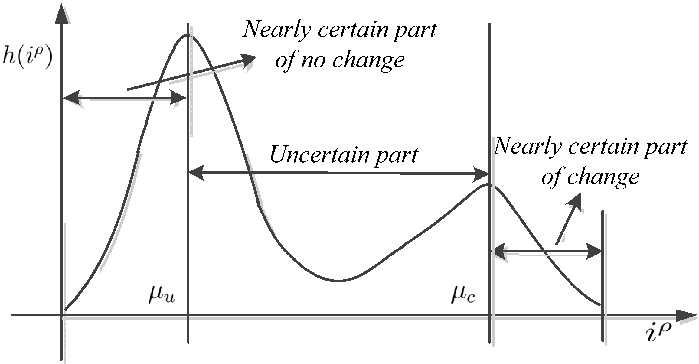
The purpose of the difference image analysis is to discriminate changed regions from unchanged regions. This process belongs to the field of image segmentation. As mentioned in Section 1, changed and unchanged classes in the difference image are not clearly defined, and an ambiguous region exists between these two classes. Therefore, we attempt to solve the change detection problem using fuzzy clustering, because fuzzy set theory [31] provides useful concepts and tools to deal with imprecise information [32]. In fuzzy clustering, difference image patterns are assigned neither to the changed nor the unchanged group but to both groups with certain membership degrees. In particular, the present work applies the properly designed RSFCM to difference image analysis, which is a variation of the standard FCM. The RSFCM description begins with a brief summary of FCM.
FCM was first introduced by Dunn [33] and was later improved by Bezdek [34]. It is an iterative clustering method that attempts to partition a finite collection of N data points into a set of C fuzzy clusters by minimizing the weighting within the group sum of the squared error objective function [25]
J ( U , V ) = n = 1 N k = 1 C u k n m d 2 ( y n , v k )
with the following constraints:
{ k = 1 C u k n = 1 0 u k n 1 n { 1 , , N }
where Y = [ y 1 , y 2 , , y N ] is the dataset to be grouped; C is the cluster number; U is the fuzzy partition matrix (membership functions), such that ukn indicates the membership grade of yn in the kth cluster; m is the weighting exponent in each fuzzy membership; V is the set of the prototypes vk associated with clusters; and d ( y n , v k ) 2 = | | y n v k | | 2 is the squared distance measure (Euclidean norm) between pattern yn and cluster center vk.
The computation of the cluster centers and membership functions is performed as follows:
v k = n = 1 N u k n m y n n = 1 N u k n m
u k n = 1 j = 1 C ( d 2 ( y n , v k ) d 2 ( y n , v j ) ) [ 1 / ( m 1 ) ]
The fuzzy partition matrix U is generally normalized, with its elements falling within [0, 1], and U and V are iteratively updated to approach an optimum solution. The iterative process ends when | | U ( r ) U ( r 1 ) | | < ε is achieved, where U ( r ) and U ( r 1 ) are the partition matrix in the rth and (r − 1)th iteration, respectively, and ε is a small positive threshold predefined manually. More details of FCM can be referenced in [34]. The dataset to be clustered in our problem is the difference image, which is divided into two groups: changed and unchanged. Therefore, N = I × J and C = 2.
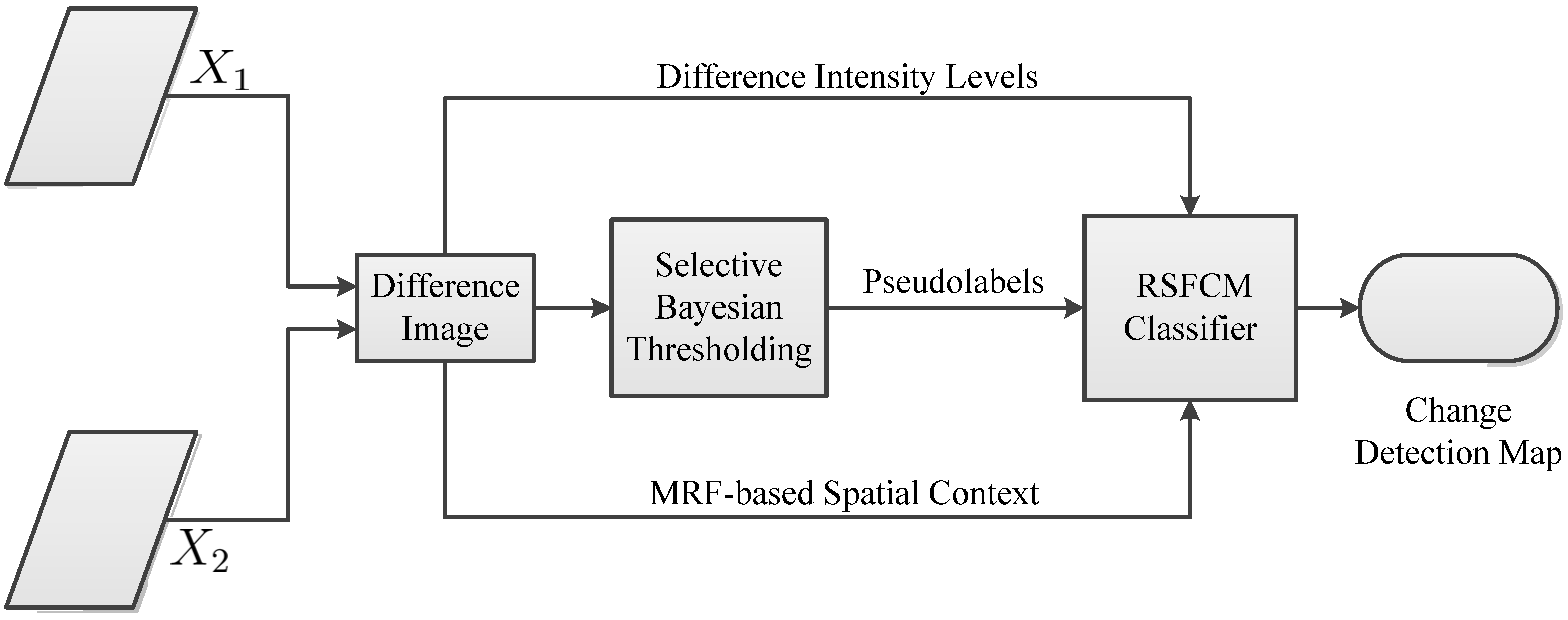
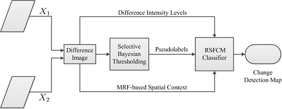
The FCM algorithm provides an appropriate tool to cluster the overlapping changed and unchanged clusters. Nevertheless, given no information on pseudolabels and spatial context, the conventional FCM only uses the difference intensity levels of the difference image pixels. We attempt to integrate these two types of valuable information into FCM to enhance the performance in change detection results, which is more difficult than when only spatial information is incorporated. Strategies to exploit labeling knowledge and information on the mutual influences among image pixels are presented in Section 2.2.2 and Section 2.2.3, respectively.

2.2.2. Strategy for Exploiting Labeling Knowledge

Several techniques have been proposed to enhance FCM performance with the help of partial supervision [29,30,35,36,37]. Bensaid and Bezdek [35] used labeled patterns as seeds to initialize the clusters’ centers. However, the potential of labeled data points has not been fully realized because they have only been used for initializing the cluster prototypes. To fully utilize this potential, labeled patterns are given more weight than the unlabeled ones in [36] when the cluster centers are calculated. Nevertheless, this approach assumes that the labeled patterns all have a correct label; the reassignment of patterns is conducted only for unlabeled patterns. This manner is inappropriate for our condition because the label set Yl, which is obtained automatically, can have noisy elements (error labels). Semi-supervised clustering algorithms based on a modified FCM objective function were discussed in [29,30,37]. These algorithms do not only fully exploit the labeled data points but are also suitable for conditions in which data is neither completely nor perfectly labeled.
Inspired by [30], we propose the approach for incorporating partial supervision into the process of analyzing the difference image, in which the problem of clustering labeled and unlabeled data is explicitly expressed as an augmented objective function. The main idea of this strategy is to use the labeled patterns (the nearly certain patterns) to guide the process of segmenting the difference image to obtain a more accurate membership. The augmented objective function consists of two components. The former is namely the FCM objective function, and it concerns unsupervised clustering. The latter retains the relationship between the pseudolabels and clusters generated by the first component.
The following is the detailed description of the proposed technique for exploiting the pseudolabels. The augmented objective function adopted assumes the following form:
J ( U , V ) = n = 1 N k = 1 C u k n m d 2 ( y n , v k ) + α n = 1 N k = 1 C ( u k n u ˜ k n ) m d 2 ( y n , v k )
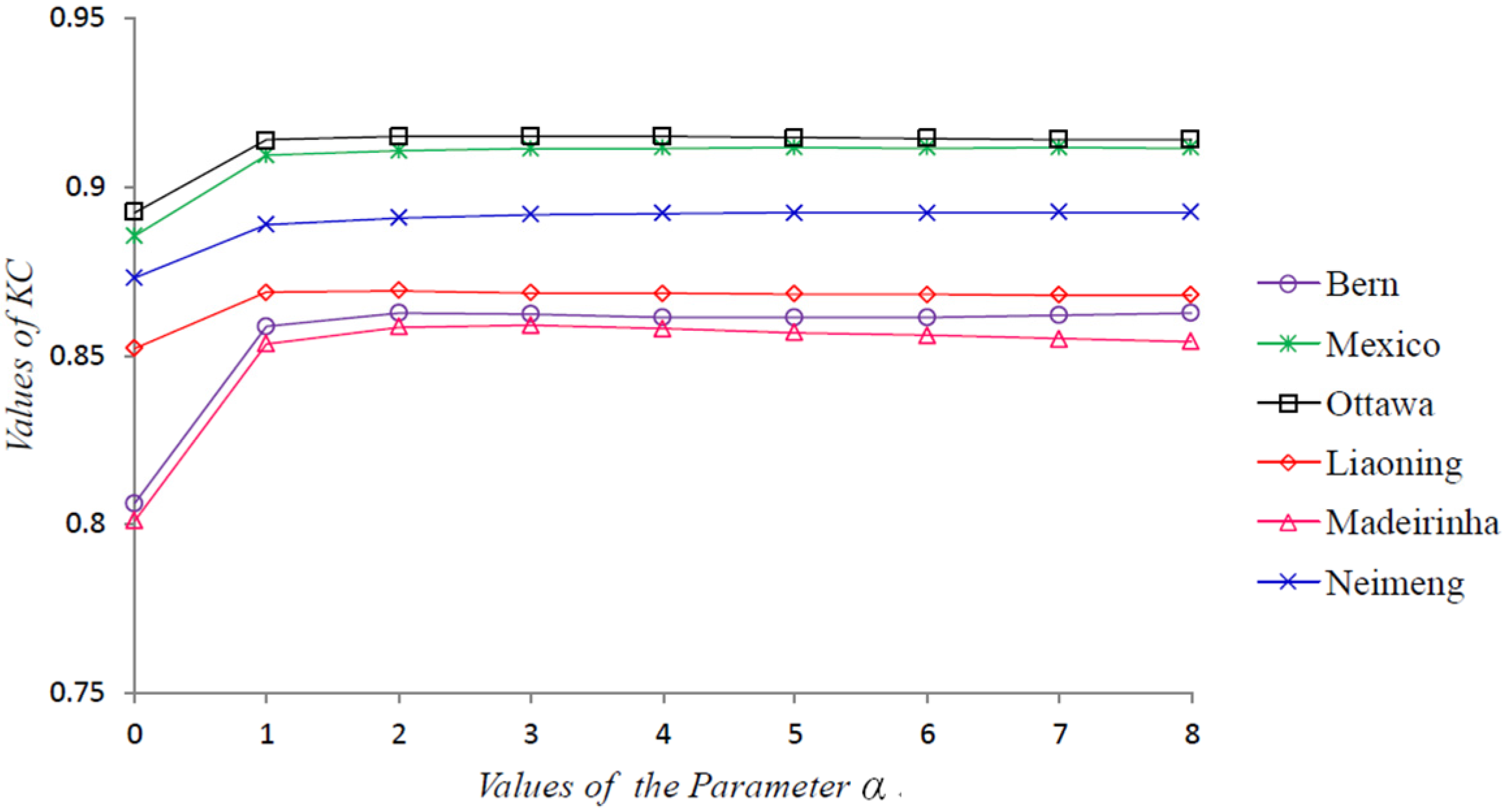
The parameter α is a scaling factor that helps establish a sound balance between the unsupervised and supervised components. Furthermore, the terms u ˜ k n are the optimal membership degrees for the labelled data points, which are derived from the labeling information contained in the set Yl. The matrix U ˜ = [ u ˜ k n ] in Equation (11) helps to optimize the membership for the difference image pixels to the changed and unchanged classes using labeling information ( u ˜ k n ) in contrast to ukn. The second (supervised) term is minimized when the value of ukn becomes close to that of u ˜ k n . Therefore, the membership value ukn is constrained to approach the corresponding u ˜ k n . Ideally, both ukn and u ˜ k n should have the same value.
Using Equation (11), both the hidden and the visible structures of the difference image can be captured. The first term attempts to discover the hidden data structure, whereas the second term considers the visible data structure reflected by the available labels (pseudolabels). The matrix U ˜ is the main part of the second component. The terms u ˜ k n are iteratively computed as follows:
u ˜ k n ( r ) = u ˜ k n ( r 1 ) η Q ( L , U ˜ ) u ˜ k n
where the superscript r refers to consecutive iterations and
Q ( L , U ˜ ) = n = 1 N k = 1 C δ n ( u ˜ k n k n ) 2 , u ˜ k n [ 0 , 1 ]
L = [ l k n ] is a C × N binary matrix used to arrange labeling information, so that l k n = 1 if pattern yn belongs to the kth class and 0 otherwise. The vector δ = [ δ n ] is two valued and specifies whether the data point n is labeled (i.e., δ n = 1 if yn is a labeled pattern and 0 otherwise). Moreover, the parameter η in Equation (12) is a positive learning rate that controls the process of updating the membership grades of U ˜ . By substituting Equation (13) into Equation (12), the learning rule Equation (12) is transformed into the following:
u ˜ k n ( r ) = u ˜ k n ( r 1 ) 2 η δ n ( u ˜ k n ( r 1 ) k n )
Equation (14) optimizes the amount u ˜ k n by exploiting the learning rate η and computed difference. U ˜ is initialized by U(°), which is obtained by applying the standard FCM to the difference image. The iterative process of computing U ˜ terminates when | | U ˜ ( r ) U ˜ ( r 1 ) | | < τ is reached, where τ is a small positive threshold. The resulting matrix U ˜ is used to compute the second term in Equation (11), the difference between U and U ˜ . The process of computing U ˜ is the same process of minimizing Q ( L , U ˜ ) .
After obtaining the matrix U ˜ , an iterative semi-supervised algorithm for minimizing Equation (11) can be derived by evaluating cluster centers and membership matrices that satisfy a zero gradient condition. For simplicity, the weighting exponent m in Equation (11) is set to 2 in this work. The calculation formulas of the cluster centers and membership functions are as follows [30]:
v k = n = 1 N ( u k n 2 + ( u k n u ˜ k n ) 2 ) y n n = 1 N ( u k n 2 + ( u k n u ˜ k n ) 2 )
u k n = α u ˜ k n ( 1 + α ) + 1 ( α / ( 1 + α ) ) s = 1 C u ˜ s n s = 1 C d 2 ( y n , v k ) / d 2 ( y n , v s )
Thus far, the utilization of labeling information (the pseudolabels) is accomplished by the terms u ˜ k n in Equations (15) and (16), and a semisupervised FCM algorithm (SFCM) is presented. However, similar to the conventional FCM, SFCM is also sensitive to noise and outliers because it does not consider information on spatial context. Moreover, the SFCM performance can be affected to a certain extent by the noisy (error) labels contained in the set Yl. Local spatial information is introduced into SFCM, as presented in Section 2.2.3, to enhance the robustness of SFCM to noise pixels and error labels.

2.2.3. Strategy for Utilizing Information on Spatial Context

This section proposes a technique for incorporating information on spatial context in SFCM, by which the RSFCM clustering algorithm is developed. The developed technique does not improve the SFCM by modifying its objective function as in [21,
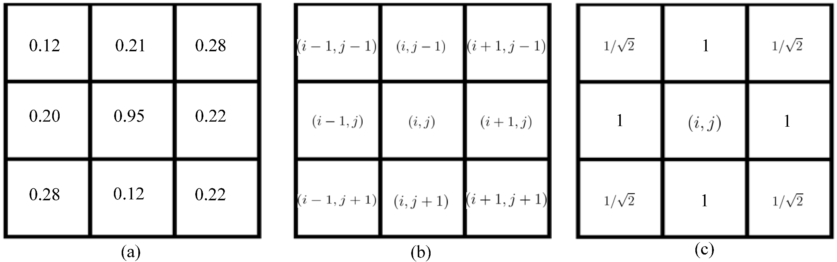
25]. Instead, it focuses on the modification of the membership in each iteration process. The aim of the modification is to discourage unlikely or undesirable configurations in the SFCM membership functions, such as a high membership value immediately surrounded by low values of the same class (Figure 3a).
A Markov random field (MRF) provides an opportune tool to introduce information on the mutual influences among image pixels in a powerful and formal manner, and it has been widely used for the change detection problem [7,12,26,38,39]. We call a random field an MRF if and only if some property of each site (pixel) is related only to the neighborhood ones and has no relationship with the other ones in a field (an image) [39]. Thus, the complexity of utilizing the spatial contextual information can be largely simplified by passing from a global model to a model of the local image properties (i.e., adopting the MRF method). An important issue of MRF model is the energy function, by which the abstract MRF expression is converted into a computable expression.
The SFCM algorithm is improved in this work based on the MRF-based spatial context, which is incorporated into the SFCM membership by adding a new spatial energy term. We then use X D ( i , j ) to denote the data points of the difference image, where (i, j) represents the pixel coordinates.
First, we present the conventional local MRF energy function because it has a basic relationship with the proposed scheme for the utilization of spatial context. The local energy function for pixel X D ( i , j ) takes on the following form [12,38,40]:
U M R F ( X D ( i , j ) ) = U s p e c t r a l ( X D ( i , j ) ) + U s p a t i a l ( X D ( i , j ) )
where U s p e c t r a l ( X D ( i , j ) ) is the spectral energy function from the observed image, and U s p a t i a l ( X D ( i , j ) ) is the spatial energy term that describes information on the mutual influences among neighboring pixels. Introducing the concept of the spatial neighborhood system is necessary to determine the spatial energy term, and the most commonly used second-order neighborhood system (Figure 3b) is adopted. The second-order neighborhood system for pixel (i, j) is denoted by N(i, j). The spatial energy term can then be defined as follows [12,38]:
U s p a t i a l ( X D ( i , j ) ) = β ( g , h ) N ( i , j ) I ( l ( i , j ) , l ( g , h ) )
The parameter β is a constant used to tune the influence of information on spatial context, and l ( i , j ) and l ( g , h ) ( ( g , h ) N ( i , j ) ) denote the class labels for the pixel (i, j) and its neighborhood, respectively. Furthermore, I ( · , · ) is an indicator function that is applied to count the number of neighborhood pixels that belong to the same class of X D ( i , j ) , which is defined as follows:
I ( l ( i , j ) , l ( g , h ) ) = { 1     i f l ( i , j ) = l ( g , h ) 0     o t h e r w i s e
On the basis of the MRF energy Equation (17), we propose the approach to improve the membership of SFCM. After calculating it in each iteration process, the SFCM membership is modified by adding a novel fuzzy spatial term. The modified membership takes on the following form:
u k , ( i , j ) M o d = u k , ( i , j ) + u k , ( i , j ) s p a t i a l
The term u k , ( i , j ) is the membership grade for the pixel (i, j) to class k computed by Equation (16), and u k , ( i , j ) s p a t i a l is the additional spatial term defined as follows.
The spatial information contained within the neighborhood centered at pixel (i, j) can be effectively used with Equation (18). However, Equation (18) is defined following classical set theory and uses the hard indicator function I ( · , · ) . Therefore, it is inappropriate for defining the spatial term u k , ( i , j ) s p a t i a l as the SFCM algorithm belongs to the family of fuzzy clustering, in which the pixels are assigned not to any one class but to all the classes with certain membership grades. Additionally, we change the influence of the pixels within the local window flexibly based on their spatial distances to reflect the damping extent of the neighborhood pixels with the spatial distance from the center pixel. Thus, to determine the degree of influence of the neighboring pixels for the center pixel, a fuzzy spatial information measure is defined based on the membership degree and distance as follows:
u k , ( i , j ) s p a t i a l = β ( g , h ) N ( i , j ) u k , ( g , h ) d ( i , j ) , ( g , h )
where u k , ( g , h ) is the membership degree for X D ( g , h ) to cluster k computed by Equation (16), d ( i , j ) , ( g , h ) is the spatial Euclidean distance (Figure 3c) between pixel (i, j) and its neighborhood ( g , h ) , and parameter β is used to control the influence of spatial information on the change detection process. Generally, different β-values can be considered. Here, we simply set the value of β to 1 as both u k , ( i , j ) and u k , ( g , h ) are the membership of SFCM calculated by Equation (16).
In expression Equation (21), we adopt the membership u k , ( · , · ) to replace the hard indicator function I ( · , · ) to describe the influence of neighboring pixels on the central pixel. The inverse distance d ( i , j ) , ( g , h ) 1 is used, as the closer the neighbors from the center (i, j) are, the more influence they exert on the result and vice versa. With the proposed fuzzy spatial term Equation (21), unlikely or undesirable configurations in the membership functions can be discouraged. For instance, if the central pixel is corrupted by noise while its neighboring pixels are homogeneous, i.e., not corrupted by noise (Figure 3a), the undesirable membership grade of the noisy (central) pixel will converge to similar neighboring pixel membership degrees because of the addition of the fuzzy spatial term Equation (21).
Eventually, we achieve a robust semi-supervised FCM algorithm called RSFCM, of which the main steps are presented in tabular form (Algorithm 1). In RSFCM, difference intensity levels and labeling information are used to estimate the membership, which is then modified by information about spatial context (as shown in Steps 3a–d of Algorithm 1). In the stage of estimating membership functions, the supervised (second) term of Equation (11) constrains the membership value ukn to approach the optimal u ˜ k n and enables the nearly certain change patterns to have a greater membership of the change class (see Step 3b), by which the change information is enhanced; in the stage of modifying the membership, the fuzzy spatial term Equation (21) discourages the undesirable configurations of membership functions caused by noise or error labels (see Step 3d), by which membership functions become spatially smooth. Therefore, RSFCM provides noise-immunity and preserves more detailed change information.
Notably, in the proposed RSFCM algorithm, the weighting exponent m is set to the value of 2 (see Equations (15) and (16)). In addition, the modified membership grades computed by Equation (20) are normalized in each iteration process, with their elements falling in [0,1].
Algorithm 1 Main steps of the RSFCM clustering algorithm
1:
The standard FCM is applied to the difference image to produce an initial partition matrix U(°).
2:
The matrix U ˜ is derived with labeling knowledge.
U ˜ is initialized with U(°) and r = 1 is set.
Repeat
   U ˜ ( r ) is computed using Equation (14).
Until | | U ˜ ( r ) U ˜ ( r 1 ) | | < τ where τ is a small positive threshold.
3:
Membership functions U are computed using intensity levels, U ˜ and spatial context.
U is initialized with U(°) and r = 1 is set.
Repeat
(a)
V (r) is computed using Equation (15).
(b)
U (r) is computed using Equation (16).
(c)
The fuzzy spatial term u k , ( i , j ) s p a t i a l is computed using Equation (21).
(d)
U (r) is modified with Equation (20).
Until | | U ( r ) U ( r 1 ) | | < ε where ε is a small positive threshold.

2.3. Implementation of the RSFCM Change Detection

In this study, a novel technique based on RSFCM is presented to analyze the difference image in the unsupervised change detection problems. The technique is an ensemble method that combines the difference intensity levels, pseudolabels and spatial context. Labeling information is used to guide the computation of membership functions, and spatial information helps to restrict membership functions to be spatially smooth. Fully exploiting the available information from the difference image guarantees the effectiveness of the RSFCM for change detection. The implementation of the RSFCM change detection method includes the following three operational steps (Figure 1):
(1)
Produce difference image
The proposed approach is based on the difference image that represents the change information. Difference images are created by applying differencing technique (as shown in Equation (1) or Equation (2)) to X1 and X2, two remotely sensed images of the same scene taken at two different times.
(2)
Identify labeled patterns (nearly certain samples)
This step is a preparatory stage to derive the nearly certain samples with a high probability to be changed or unchanged class, of which the pseudolabels are used by RSFCM to guide the clustering of the difference image. The nearly certain patterns are identified by applying two adequate thresholds induced by the Bayesian threshold to the histogram of the difference image. Details of the process can be found in Section 2.1.
(3)
Distinguish changed regions from unchanged regions
In this step, the change detection map is generated by labeling the difference image pixels into changed and unchanged classes. First, the difference image is partitioned into two fuzzy clusters by calculating the fuzzy partition matrix U = [ u k , ( i , j ) ] using the properly designed RSFCM algorithm. Then, a defuzzification process takes place to convert the fuzzy partition matrix U to a crisp partition. The maximum membership procedure is the most important approach developed to defuzzify U [25]. In this study, this procedure is adopted to convert the fuzzy difference image achieved by RSFCM to the change detection map. It assigns the pixel X D ( i , j ) to the class w k with the higher membership
w k = a r g k { m a x { u k , ( i , j ) } }     w k = w u o r w c .

3. Experiments and Analysis

3.1. Dataset Description and Experimental Settings

3.1.1. Datasets

To evaluate the effectiveness of the proposed change detection approach, six real multitemporal remotely sensed datasets acquired by different sensors referring to different changes were considered in the experiments. Typical corrections, such as co-registration and relative radiometric correction, were done on the six used remote sensing datasets before applying the proposed change detection approach. The first three datasets shown in Figure 4 are available from [41]. The information regarding the north direction and detailed location of these three datasets could not be made available from [41]. The other three datasets with their detailed location information are shown in Figure 5. Reference data (ground truth) is always a problem for accuracy assessment of land cover change detection; inaccurate reference data will lead to an improper assessment result. In this study, the reference images were created manually based on a detailed visual analysis of the two original images and their difference images using ENVI.
The first dataset is the Bern dataset, which represents a section (301 × 301 pixels) of two SAR images acquired by the European Remote Sensing 2 satellite SAR sensor over an area near the city of Bern in April 1999 and May 1999. The Aare Valley between Thun and Bern was selected as a test area given that the River Aare flooded parts of Thun and Bern as well as the Bern airport entirely between these two dates. Figure 4a–c shows the images and the corresponding ground truth.
The second dataset, the Mexico dataset, represents a section (512 × 512 pixels) of two optical images acquired by the Landsat ETM+ sensor over an area of Mexico on 18 April 2000 and 30 May 2002. Between the two acquisition dates, fire destroyed a large portion of vegetation in the considered region. Figure 4d,e shows channel 4 of the April and May images, respectively, and Figure 4f shows the ground truth of the second dataset.
The third dataset is called the Ottawa dataset, which is a section (290 × 350 pixels) of two SAR images acquired by the Radarsat SAR sensor over the city of Ottawa in July 1997 and August 1997. These images contain roughly two regions: land and water. The images and the available ground truth are shown in Figure 4g–i, respectively.
The dataset used in the fourth experiment is the Liaoning dataset, which comprises two Landsat 7 ETM+ images acquired in August 2001 and August 2002 in Liaoning Province, China. The area selected for the experiments is a section with a size of 400 × 400 pixels. Figure 5a–c shows channel 4 of the two images and the available ground truth.
The dataset used in the fifth experiment is the Madeirinha dataset composed of two Landsat TM images with a size of 400 × 400 pixels acquired in July 2000 and July 2006 near Madeirinha, Brazil. Figure 5d–f shows band 3 of the images and the ground truth of the fifth dataset, respectively.
The dataset used in the sixth experiment is the Neimeng dataset (400 × 400 pixels), which was acquired by Landsat 5 TM in August 2007 and 2010 in Neimeng Province, China. Figure 5g–i shows channel 7 of the two images and the corresponding ground truth.

3.1.2. Compared Algorithms and Evaluation Criteria

To evaluate the effectiveness of the proposed RSFCM change detection approach, experiments were conducted on the six different remote sensing datasets. Performance of the proposed technique was compared with those of five known algorithms. The first compared algorithm is the EM algorithm, which serves as the basis for identifying labeled pixels for the RSFCM approach. The second compared algorithm is the EMMRF algorithm, where EM was combined with MRF [12]. The algorithm increases the accuracy of the final change detection map from EM by exploiting the spatial context by the traditional MRF spatial Equation (18).
The third, fourth, and fifth compared algorithms belong to the FCM algorithm family. The third compared algorithm, which is the standard FCM, is the most basic member of the family. This experiment was conducted to demonstrate whether adding information on the spatial context would yield better results. The fourth and fifth compared algorithms are the FLICM [25] and RFLIFCM [21], respectively. Both of them are state-of-the-art context-sensitive FCM algorithms. The two experiments were designed to prove whether adding labeling information will yield better change detection results and the low time complexity of RSFCM.
In addition, to show the effect of using labeling knowledge on the RSFCM change detection results, we provide the results produced by a special RSFCM (called sRSFCM), which does not consider any labeling information. In particular, the parameter α used to control the influence of labeling information is set to 0 in the sRSFCM algorithm.
Both qualitative and quantitative analyses were made on the experimental results. In the qualitative (visual) analysis, we compared the binary change detection map of each algorithm with the binary ground truth image. For quantitative analysis, four accuracy indices were computed for each change detection map: (1) miss detection (MD); (2) false alarms (FA); (3) overall error (OE); and (4) Kappa coefficient (KC) [16,42].
In addition, the time T consumed in the whole process is also an important criterion. T was recorded to compare the time complexity of different algorithms, and the unit used is the second. The computation time analyses were performed on a computer with an Intel(R) Core (TM) i5-2400 3.1 GHz processor and 4 GB RAM.

3.2. Experimental Results

The EM algorithm is free from using any parameters, and the EMMRF algorithm depends on the parameter β that tunes the influence of spatial contextual information. The FCM, FLICM, and RFLICM use the value of weighting exponent m to control the degree of fuzziness in the resulting membership functions. For the proposed RSFCM, the parameter m is set to 2 (see Equations (15) and (16)). RSFCM uses the parameter α to adjust the contribution of labeling information. In this study, various parameter values of the algorithms were experimentally explored, and only the best change detection results are presented for performance evaluation and illustration. In the following, we first present the test of the parameter α of RSFCM and then the results on the six remotely sensed datasets.

3.2.1. Test of the Parameter α

This section tests the parameter α, which is used by RSFCM to adjust the influence of labeling knowledge. The parameter α was tested because we wanted to know its effect on the RSFCM change detection results and attempted to find a reasonable range (or value) for which better results could be achieved. In this test, the parameter α ranges from 0 to 8 and includes certain discrete values. The six datasets were experimented on, and the reliable and cogent criterion KC was used. Figure 6 shows the testing results on the six datasets. In particular, the α-value 0, which corresponds to an unsupervised RSFCM algorithm (i.e., the sRSFCM), serves as a comparison point for the test.
Based on the six curves, the value of KC increases conspicuously when the α-value changes from 0 to 1, whereas the KC value nearly stays constant in all the datasets when the α-value is larger than 1. The noticeable increase indicates that the utilization of labeling knowledge can significantly improve the performance of RSFCM. Moreover, the stability of KC under various α-values in the range of 1–8 shows that RSFCM is robust. That is, one can select any value in the range [1,2,3,4,5,6,7,8] for a reasonable performance of RSFCM for all the six datasets.
In subsequent case studies, the change detection results with the optimal α-value are presented for performance evaluation. The α-values used in the first to the sixth experiments are 2, 4, 3, 2, 4, and 1, respectively.

3.2.2. Experiment Results and Analysis

Performance studies were conducted based on the best results of the algorithms obtained by altering their parameters. The results are exhibited in two ways: the final maps in graphic format and the evaluation criteria in a tabular format. The change detection maps obtained from the six algorithms on the Bern, Mexico, Ottawa, Liaoning, Madeirinha, and Neimeng datasets are shown in Figure 7, Figure 8, Figure 9, Figure 10, Figure 11 and Figure 12, respectively. In order to clearly show the difference of the change map compared to the corresponding ground truth, each map is partitioned into four parts in different colors: black denotes the unchanged pixels that are detected correctly, yellow the FA pixels, red the MD pixels, and white the correctly detected change pixels. The four accuracy indices (MD, FA, OE, and KC) of each map and computation times on the six datasets are depicted in Table 1, Table 2, Table 3, Table 4, Table 5 and Table 6, respectively.
The visual comparison between the generated change maps and corresponding ground truths gives a rough idea about the quality of each of these maps.
As shown in Figure 7, Figure 8, Figure 9, Figure 10, Figure 11 and Figure 12, six methods provide different change maps over the same geographical area. The change detection maps yielded by EM contain many yellow noise spots (Figure 7, Figure 8, Figure 9, Figure 10, Figure 11 and Figure 12a) and have the largest (worst) FA (Table 1, Table 2, Table 3, Table 4, Table 5 and Table 6). This is mainly because EM fails to consider any information on the spatial context in the process of the difference image analysis. By incorporating the information provided by the neighboring pixels, the EMMRF algorithm greatly improves the EM change detection results. Most of the noise is removed (Figure 7, Figure 8, Figure 9, Figure 10, Figure 11 and Figure 12b), and the value of FA significantly decreases (Table 1, Table 2, Table 3, Table 4, Table 5 and Table 6). As an example, for the Bern data, the FA value decreases from 4785 to 1088 (Table 1). However, the detecting results from the EMMRF are still not satisfactory enough compared to the reference maps (Figure 7, Figure 8, Figure 9, Figure 10, Figure 11 and Figure 12b). The two major reasons for this are that, (1) EMMRF is a post-processing of the EM change detection, and its results depend on the EM results; and (2) the EMMRF algorithm (similar to EM) is developed based on the classical set theory and does not work well on separating the overlapping unchanged and changed clusters.
Benefiting from the fuzzy set theory, FCM produces better change detection results than the context-insensitive EM for all the six case studies (Figure 7, Figure 8, Figure 9, Figure 10, Figure 11 and Figure 12 and Table 1, Table 2, Table 3, Table 4, Table 5 and Table 6). It also performs better than the context-sensitive EMMRF algorithm for the Bern, Liaoning and Neimeng datasets in terms of OE and KC (Table 1, Table 4, and Table 6). Nevertheless, the change detection maps from FCM still contain much noise (Figure 7, Figure 8, Figure 9, Figure 10, Figure 11 and Figure 12c). Moreover, FCM produces the highest (or nearly highest) MD value, thus proving that the use of spatial context positively affects the change detection results. Through incorporating information about the spatial context, change detection maps obtained by FLICM (Figure 7, Figure 8, Figure 9, Figure 10, Figure 11 and Figure 12d) and RFLICM (Figure 7, Figure 8, Figure 9, Figure 10, Figure 11 and Figure 12e) are robust to noise and almost all the yellow noise spots on the FCM change maps are eliminated. The results from FLICM and RFLICM are better than those of EMMRF and even better than those of sRSFCM (that is, the special case of RSFCM in which no labeling information is considered). However, similar to the standard FCM, FLICM and RFLICM overlook some vital change regions. This can be seen from the (large) red area for MD pixels contained in their change maps. This is mainly because, FLICM and RFLICM algorithms are intended to improve FCM robustness to noise and outliers, and they only consider information on the spatial context. The use of spatial information may lead to over smoothing on the boundaries of change regions (Figure 7, Figure 10, and Figure 11).
Different from FLICM and RFLICM, RSFCM synergistically exploits both the spatial context and pseudolabels to improve the FCM performance. RSFCM uses spatial context to modify the membership by the improved MRF Model (21), and thus the unlikely configurations of membership functions are discouraged. As a result, almost all the scattering of yellow false alarms in FCM change maps are removed (Figure 7, Figure 8, Figure 9, Figure 10, Figure 11 and Figure 12f). Also, the use of labeling knowledge (pseudolabels) by a supervised component makes the nearly certain change patterns have a greater membership of change category, hence enhancing the change information. The red area of the RSFCM maps is thus significantly reduced and the missed detecting problem is noticeably solved in RSFCM (Figure 7, Figure 8, Figure 9, Figure 10, Figure 11 and Figure 12). Figure 13 and Figure 14 present close-up shots of the change maps generated by FCM, FLICM, RFLICM, sRSFCM, and RSFCM on the Mexico and Madeirinha datasets, from which the advantage of RSFCM on solving the missed detection problem can be clearly seen. Consequently, the proposed RSFCM can both tolerate noise and preserve more change information, producing the most accurate change maps (Figure 7, Figure 8, Figure 9, Figure 10, Figure 11 and Figure 12g).
The quantitative superiority of the proposed method can be seen from Table 1, Table 2, Table 3, Table 4, Table 5 and Table 6. RSFCM yields the best values of both OE and KC for all the six experiments. For example, for the Mexico data, RSFCM produces the smallest OE of 4047 pixels, with differences of 7074, 1312, 1516, 815, and 762 pixels compared with EM, EMMRF, FCM, FLICM, and RFLICM, respectively; the KC of RSFCM is 0.9117, which is 12.16%, 2.05%, 3.59%, 2.14%, and 2.02% larger than that of EM, EMMRF, FCM, FLICM, and RFLICM, respectively.
As indicated in Table 1, Table 2, Table 3, Table 4, Table 5 and Table 6, only RSFCM obtains both lower (better) FA and MD compared with FCM for all the six datasets, quantitatively confirming that RSFCM not only minimizes the noise but also preserves more change information. Compared with FLICM and RFLICM, our technique provides a noticeable reduction in the MD error for all the six experiments, a comparable value in the FA error for the Bern, Mexico, Liaoning, and Madeirinha datasets, and a higher FA for the Ottawa and Neimeng datasets. As shown in Figure 9 and Figure 12, the higher FA makes the RSFCM change maps contain more noise than those of FLICM and RFLICM. However, the OE and KC values of RSFCM for the Ottawa and Neimeng datasets are better than those of FLICM and RFLICM (the results obtained by RFLICM are comparable to the RSFCM results on the Ottawa dataset), thus RSFCM still yields change maps closer to ground truth.
To make a more objective evaluation of the performance of the proposed method, the average results from the six datasets of each method were computed. Here the overall evaluation criterions OE and KC and the computation time T were considered. Figure 15 plots the average OE, KC and T obtained from the six methods. As can be seen, our technique produces significant reductions in the average OE change detection error and increases in the average KC compared with other methods. The comparison result of the average OE and KC confirms that the performance of RSFCM is superior to those of the other five algorithms. As regards the computation time complexity, the proposed method has slightly higher (average) computation time requirement than the EM, EMMRF, and FCM methods. Moreover, it only requires approximately one-third of the computational times of FLICM and RFLICM.
The experimental results show that, in all cases and on average, the proposed RSFCM technique outperforms the other approaches (although the results obtained by the RFLICM are comparable to the RSFCM results on the Ottawa dataset, RFLICM requires much more computation time than RSFCM). The approach is capable of guaranteeing noise insensitiveness and preserving more change information. Moreover, it can fit different types of remotely sensed images and is low in time complexity.

4. Conclusions

In this study, we have proposed a novel unsupervised change detection approach in multitemporal remote sensing images based on a properly designed RSFCM algorithm. The main idea of this method is to combine the three types of valuable information from the difference image: (a) intensity levels, (b) labeling knowledge, and (c) spatial information. First, the problem of deriving the labeled patterns (the nearly certain pixels) from the difference image is solved by determining two appropriate thresholds for the difference image histogram based on the Bayes theory. Then, via a supervised component and a fuzzy spatial term, RSFCM incorporates labeling knowledge and information on spatial context into the FCM, respectively, which mainly uses the gray-level intensity. The former is used to supervise the clustering process of the difference image for enhancing change information and achieving more accurate membership, and the latter is used to modify the membership for obtaining spatially smooth membership functions and thus reducing the effect of noise pixels and error labels. Therefore, the change detection map produced by the RSFCM is not only robust to outliers but also contains more change information.
Six experiments were conducted on different remotely sensed images to evaluate the performance of the RSFCM. Compared with EM, EMMRF, FCM, FLICM, and RFLICM, RSFCM performs better in both qualitative and quantitative measures. Moreover, RSFCM is low in time complexity. These qualities verify the effectiveness and efficiency of RSFCM. Furthermore, the experimental results indicate that RSFCM can fit different types of remote sensing images, such as TM and SAR images, which can refer to different kinds of changes and have different degrees of noise.
Theoretically, this study contributes to the development of change detection by proposing the idea of combining difference intensity levels, labeling knowledge, and spatial information from the difference image. Methodologically, it presents a method to automatically derive labeled patterns from the difference image, develops a novel algorithm (RSFCM) for image segmentation, and defines a change detection framework.
Notably, in the first step of the proposed change detection approach, other thresholding algorithms such as Kapur can be used to take the place of EM for obtaining nearly certain pixel-patterns. In the second step, some universal models such as the spatial attraction model can be used to define the fuzzy spatial term for modifying the membership.
In our future investigations, additional work will be conducted on the methods of determining the fuzzy spatial term, and RSFCM will be applied to other types of remotely sensed images, among others.

Acknowledgments

The authors would like to thank Anshu Zhang for checking the English, Maoguo Gong for providing the first three used datasets. We are also grateful to the editors and anonymous reviewers for their valuable comments and helpful suggestions, which greatly improved the quality of this paper. This work was supported by the National Natural Science Foundation of China (Project No.: 213210700070 and 41331175), the Ministry of Science and Technology of China (Project No.: 2012BAJ15B04), the Hong Kong Polytechnic University (Project No.: 1_ZVF2 and 1-ZVE8), and Hong Kong Innovation & Technology Fund (Project No.: 1-ZEA5).

Author Contributions

Pan Shao and Wenzhong Shi proposed the original idea and designed the study. Pan Shao performed the experiments and analyzed the data. Ming Hao, Pengfei He and Xiaokang Zhang contributed significantly to the discussion of the results. Pan Shao wrote the manuscript which was revised by all authors.

Conflicts of Interest

The authors declare no conflict of interest.

References

  1. Singh, A. Digital change detection techniques using remotely-sensed data. Int. J. Remote Sens. 1989, 10, 989–1003. [Google Scholar] [CrossRef]
  2. Lu, D.; Mausel, P.; Brondizio, E.; Moran, E. Change detection techniques. Int. J. Remote Sens. 2004, 25, 2365–2401. [Google Scholar] [CrossRef]
  3. Radke, R.J.; Andra, S.; Al-Kofahi, O.; Roysam, B. Image change detection algorithms: A systematic survey. IEEE Trans. Image Process. 2005, 14, 294–307. [Google Scholar] [CrossRef] [PubMed]
  4. Bruzzone, L.; Bovolo, F. A novel framework for the design of change-detection systems for very-high-resolution remote sensing images. Proc. IEEE 2013, 101, 609–630. [Google Scholar] [CrossRef]
  5. Hussain, M.; Chen, D.; Cheng, A.; Wei, H.; Stanley, D. Change detection from remotely sensed images: From pixel-based to object-based approaches. ISPRS J. Photogramm. Remote Sens. 2013, 80, 91–106. [Google Scholar] [CrossRef]
  6. Tewkesbury, A.P.; Comber, A.J.; Tate, N.J.; Lamb, A.; Fisher, P.F. A critical synthesis of remotely sensed optical image change detection techniques. Remote Sens. Environ. 2015, 160, 1–14. [Google Scholar] [CrossRef]
  7. Melgani, F.; Bazi, Y. Markovian fusion approach to robust unsupervised change detection in remotely sensed imagery. IEEE Geosci. Remote Sens. Lett. 2006, 3, 457–461. [Google Scholar] [CrossRef]
  8. Gong, M.; Li, Y.; Jiao, L.; Jia, M.; Su, L. SAR change detection based on intensity and texture changes. ISPRS J. Photogramm. Remote Sens. 2014, 93, 123–135. [Google Scholar] [CrossRef]
  9. Chen, J.; Lu, M.; Chen, X.; Chen, J.; Chen, L. A spectral gradient difference based approach for land cover change detection. ISPRS J. Photogramm. Remote Sens. 2013, 85, 1–12. [Google Scholar] [CrossRef]
  10. Almutairi, A.; Warner, T.A. Change detection accuracy and image properties: A study using simulated data. Remote Sens. 2010, 2, 1508–1529. [Google Scholar] [CrossRef]
  11. Roy, M.; Ghosh, S.; Ghosh, A. A novel approach for change detection of remotely sensed images using semi-supervised multiple classifier system. Inform. Sci. 2014, 269, 35–47. [Google Scholar] [CrossRef]
  12. Bruzzone, L.; Prieto, D.F. Automatic analysis of the difference image for unsupervised change detection. IEEE Trans. Geosci. Remote Sens. 2000, 38, 1171–1182. [Google Scholar] [CrossRef]
  13. Patra, S.; Ghosh, S.; Ghosh, A. Histogram thresholding for unsupervised change detection of remote sensing images. Int. J. Remote Sens. 2011, 32, 6071–6089. [Google Scholar] [CrossRef]
  14. Zhang, P.; Shi, W.; Wong, M.S.; Chen, J. A reliability-based multi-algorithm fusion technique in detecting changes in land cover. Remote Sens. 2013, 5, 1134–1151. [Google Scholar] [CrossRef]
  15. Byun, Y.; Han, Y.; Chae, T. Image fusion-based change detection for flood extent extraction using bi-temporal very high-resolution satellite images. Remote Sens. 2015, 7, 10347–10363. [Google Scholar] [CrossRef]
  16. Bovolo, F.; Bruzzone, L.; Marconcini, M. A novel approach to unsupervised change detection based on a semisupervised SVM and a similarity measure. IEEE Trans. Geosci. Remote Sens. 2008, 46, 2070–2082. [Google Scholar] [CrossRef]
  17. Hao, M.; Shi, W.; Zhang, H.; Li, C. Unsupervised change detection with expectation-maximization-based level set. IEEE Geosci. Remote Sens. Lett. 2014, 11, 210–214. [Google Scholar] [CrossRef]
  18. Celik, T.; Ma, K.K. Unsupervised change detection for satellite images using dual-tree complex wavelet transform. IEEE Trans. Geosci. Remote Sens. 2010, 48, 1199–1210. [Google Scholar] [CrossRef]
  19. Ghosh, S.; Roy, M.; Ghosh, A. Semi-supervised change detection using modified self-organizing feature map neural network. Appl. Soft Comput. 2014, 15, 1–20. [Google Scholar] [CrossRef]
  20. Ghosh, A.; Mishra, N.S.; Ghosh, S. Fuzzy clustering algorithms for unsupervised change detection in remote sensing images. Inform. Sci. 2011, 181, 699–715. [Google Scholar] [CrossRef]
  21. Gong, M.; Zhou, Z.; Ma, J. Change detection in synthetic aperture radar images based on image fusion and fuzzy clustering. IEEE Trans. Image Process. 2012, 21, 2141–2151. [Google Scholar] [CrossRef] [PubMed]
  22. Ma, W.; Jiao, L.; Gong, M.; Li, C. Image change detection based on an improved rough fuzzy C-means clustering algorithm. Int. J. Mach. Learn. Cybern. 2014, 5, 369–377. [Google Scholar] [CrossRef]
  23. Mishra, N.S.; Ghosh, S.; Ghosh, A. Fuzzy clustering algorithms incorporating local information for change detection in remotely sensed images. Appl. Soft Comput. 2012, 12, 2683–2692. [Google Scholar] [CrossRef]
  24. Ma, J.; Gong, M.; Zhou, Z. Wavelet fusion on ratio images for change detection in SAR images. IEEE Geosci. Remote Sens. Lett. 2012, 9, 1122–1126. [Google Scholar] [CrossRef]
  25. Krinidis, S.; Chatzis, V. A robust fuzzy local information C-means clustering algorithm. IEEE Trans. Image Process. 2010, 19, 1328–1337. [Google Scholar] [CrossRef] [PubMed]
  26. Kasetkasem, T.; Varshney, P.K. An image change detection algorithm based on markov random field models. IEEE Trans. Geosci. Remote Sens. 2002, 40, 1815–1823. [Google Scholar] [CrossRef]
  27. Bovolo, F.; Camps-Valls, G.; Bruzzone, L. A support vector domain method for change detection in multitemporal images. Pattern Recognit. Lett. 2010, 31, 1148–1154. [Google Scholar] [CrossRef]
  28. Shah-Hosseini, R.; Homayouni, S.; Safari, A. A hybrid kernel-based change detection method for remotely sensed data in a similarity space. Remote Sens. 2015, 7, 12829–12858. [Google Scholar] [CrossRef]
  29. Bouchachia, A.; Pedrycz, W. A semi-supervised clustering algorithm for data exploration. In Fuzzy Sets and Systems—IFSA 2003; Bilgiç, T., de Baets, B., Kaynak, O., Eds.; Springer: Berlin, Germany; Heidelberg, Germany, 2003; Volume 2715, pp. 328–337. [Google Scholar]
  30. Bouchachia, A.; Pedrycz, W. Enhancement of fuzzy clustering by mechanisms of partial supervision. Fuzzy Sets Syst. 2006, 157, 1733–1759. [Google Scholar] [CrossRef]
  31. Zadeh, L.A. Fuzzy sets. Inf. Control 1965, 8, 338–353. [Google Scholar] [CrossRef]
  32. Wang, F. Fuzzy supervised classification of remote sensing images. IEEE Trans. Geosci. Remote Sens. 1990, 28, 194–201. [Google Scholar] [CrossRef]
  33. Dunn, J.C. A fuzzy relative of the ISODATA process and its use in detecting compact well-separated clusters. J. Cybern. 1974, 3, 32–57. [Google Scholar] [CrossRef]
  34. Bezdek, J.C. Pattern Recognition with Fuzzy Objective Function Algorithms; Plenum Press: New York, NY, USA, 1981. [Google Scholar]
  35. Bensaid, A.M.; Bezdek, J.C. Partial supervision based on point-prototype clustering algorithms. In Proceedings of the 4th European Congress on Intelligent Techniques and Soft Computing, Aachen, Germany, 2–5 September 1996; pp. 1402–1406.
  36. Bensaid, A.M.; Hall, L.O.; Bezdek, J.C.; Clarke, L.P. Partially supervised clustering for image segmentation. Pattern Recognit. 1996, 29, 859–871. [Google Scholar] [CrossRef]
  37. Yasunori, E.; Yukihiro, H.; Makito, Y.; Sadaaki, M. On semi-supervised fuzzy c-means clustering. In Proceedings of the IEEE 2009 International Conference on Fuzzy Systems, Jeju Island, Korea, 20–24 August 2009; pp. 1119–1124.
  38. Tarabalka, Y.; Fauvel, M.; Chanussot, J.; Benediktsson, J.A. SVM- and MRF-based method for accurate classification of hyperspectral images. IEEE Geosci. Remote Sens. Lett. 2010, 7, 736–740. [Google Scholar] [CrossRef]
  39. Gong, M.; Su, L.; Jia, M.; Chen, W. Fuzzy clustering with a modified MRF energy function for change detection in synthetic aperture radar images. IEEE Trans. Fuzzy Syst. 2014, 22, 98–109. [Google Scholar] [CrossRef]
  40. Hao, M.; Zhang, H.; Shi, W.; Deng, K. Unsupervised change detection using fuzzy c-means and MRF from remotely sensed images. Remote Sens. Lett. 2013, 4, 1185–1194. [Google Scholar] [CrossRef]
  41. The Title in the 2013 Intelligence Cup Programming Contest: Designing Remote Sensing Change Detection System. Available online: http://see.xidian.edu.cn/faculty/mggong/Projects/iCD.htm (accessed on 8 May 2014). (In Chinese)
  42. Foody, G.M. Status of land cover classification accuracy assessment. Remote Sens. Environ. 2002, 80, 185–201. [Google Scholar] [CrossRef]
Figure 1. Flowchart of proposed change detection approach based on robust semi-supervised fuzzy C-means (RSFCM).
Remotesensing 08 00264 g001
Figure 2. Examples of difference image histogram h ( i ρ ) and definitions of uncertain and nearly certain parts.
Remotesensing 08 00264 g002
Figure 3. (a) Example of an undesirable configuration of membership; (b) Second-order neighborhood system of pixel (i, j); (c) Distances between center pixel (i, j) and its neighbors.
Remotesensing 08 00264 g003
Figure 4. (a) Image acquired in April 1999; (b) Image acquired in May 1999; (c) Ground truth of (a,b); (d) Band 4 of image acquired in April 2000; (e) Band 4 of image acquired in May 2002; (f) Ground truth of (d,e); (g) Image acquired in July 1997; (h) Image acquired in August 1997; (i) Ground truth of (g,h).
Remotesensing 08 00264 g004
Figure 5. (a) Band 4 of image acquired in August 2001; (b) Band 4 of image acquired in August 2002; (c) Ground truth of (a,b); (d) Band 3 of image acquired in July 2000; (e) Band 3 of image acquired in July 2006; (f) Ground truth of (d,e); (g) Band 7 of image acquired in August 2007; (h) Band 7 of image acquired in August 2010; (i) Ground truth of (g,h).
Remotesensing 08 00264 g005
Figure 6. Testing curves of parameter α on six remote sensing datasets.
Remotesensing 08 00264 g006
Figure 7. Final change detection maps of the Bern dataset produced by (a) EM; (b) EMMRF; (c) FCM; (d) FLICM; (e) RFLICM; (f) sRSFCM (special case of RSFCM); (g) proposed RSFCM; and (h) reference image.
Remotesensing 08 00264 g007
Figure 8. Final change detection maps of the Mexico dataset produced by (a) EM; (b) EMMRF; (c) FCM; (d) FLICM; (e) RFLICM; (f) sRSFCM; (g) proposed RSFCM; and (h) reference image.
Remotesensing 08 00264 g008
Figure 9. Final change detection maps of the Ottawa dataset produced by (a) EM; (b) EMMRF; (c) FCM; (d) FLICM; (e) RFLICM; (f) sRSFCM; (g) proposed RSFCM; and (h) reference image.
Remotesensing 08 00264 g009
Figure 10. Final change detection maps of the Liaoning dataset produced by (a) EM; (b) EMMRF; (c) FCM; (d) FLICM; (e) RFLICM; (f) sRSFCM; and (g) proposed RSFCM; and (h) reference image.
Remotesensing 08 00264 g010
Figure 11. Final change detection maps of the Madeirinha dataset produced by (a) EM; (b) EMMRF; (c) FCM; (d) FLICM; (e) RFLICM; (f) sRSFCM; (g) proposed RSFCM; and (h) reference image.
Remotesensing 08 00264 g011
Figure 12. Final change detection maps of the Neimeng dataset produced by (a) EM; (b) EMMRF; (c) FCM; (d) FLICM; (e) RFLICM; (f) sRSFCM; (g) proposed RSFCM; and (h) reference image.
Remotesensing 08 00264 g012
Figure 13. Close-up shot of Mexico data (a) FCM; (b) FLICM; (c) RFLICM; (d) sRSFCM; and (e) RSFCM.
Remotesensing 08 00264 g013
Figure 14. Close-up shot of Madeirinha data (a) FCM; (b) FLICM; (c) RFLICM; (d) sRSFCM; and (e) RSFCM.
Remotesensing 08 00264 g014
Figure 15. Average results from different datasets (a) OE values; (b) KC values; and (c) computation times T.
Remotesensing 08 00264 g015
Table 1. Change detection results on Bern dataset.
BernMDFAOEKCT/s
EM59478548440.29661.2
EMMRF41108811290.65803.4
FCM3902826720.69893.0
FLICM284883720.82196.2
RFLICM2421053470.83836.5
sRSFCM354263800.80623.2
RSFCM213832960.86303.8
Table 2. Change detection results on Mexico dataset.
MexicoMDFAOEKCT/s
EM1329979211,1210.79011.8
EMMRF784457553590.89125.3
FCM3632193155630.87583.4
FLICM3576128648620.890318.7
RFLICM3538127148090.891518.8
sRSFCM409090149910.88565.2
RSFCM2238180940470.91175.6
Table 3. Change detection results on Ottawa dataset.
OttawaMDFAOEKCT/s
EM1417903010,4470.67581.3
EMMRF602236329650.89503.5
FCM2765215849230.81501.5
FLICM245029627460.89258.2
RFLICM177156023310.91108.5
sRSFCM245329427470.89243.6
RSFCM145680022560.91513.9
Table 4. Change detection results on Liaoning dataset.
LiaoningMDFAOEKCT/s
EM22711053312,8040.76391.5
EMMRF1924847410,3980.80453.4
FCM4692229269840.85332.4
FLICM4941187468150.855712.5
RFLICM4891186167520.857012.7
sRSFCM5224140666300.85213.3
RSFCM4320191762370.86913.8
Table 5. Change detection results on Madeirinha dataset.
MadeirinhaMDFAOEKCT/s
EM2305657788820.78282.3
EMMRF1590414157310.85545.4
FCM4229267169000.81185.9
FLICM5616127168870.801116.7
RFLICM5124145565790.812717.5
sRSFCM589789567920.80116.8
RSFCM3348194352910.85897.2
Table 6. Change detection results on Neimeng dataset.
NeimengMDFAOEKCT/s
EM146716,98918,4560.80964.3
EMMRF81312,54513,3580.85587.7
FCM9134280411,9380.85716.5
FLICM8020186198810.875122.5
RFLICM7740190396430.879823.8
sRSFCM8132197810,1100.87328.2
RSFCM6319278491030.89218.6

