
Integrated Analysis of Productivity and Biodiversity in a Southern Alberta Prairie

 and
and
Abstract
:
1. Introduction
2. Methods
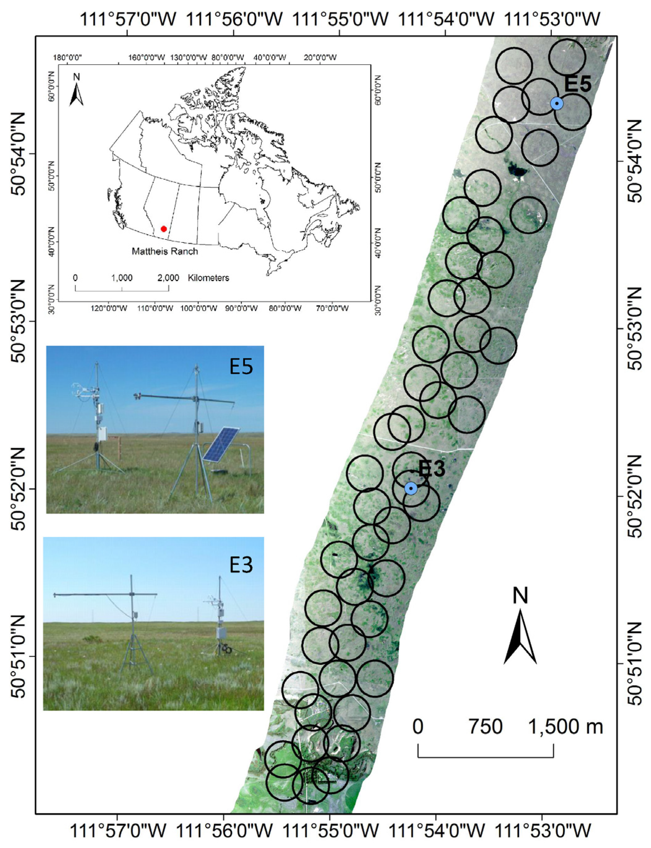
2.1. Study Site
2.2. Optical Phenology and Flux Measurements
2.3. Biomass Harvest
2.4. APAR Determination
2.5. Ground NDVI
2.6. Airborne Data
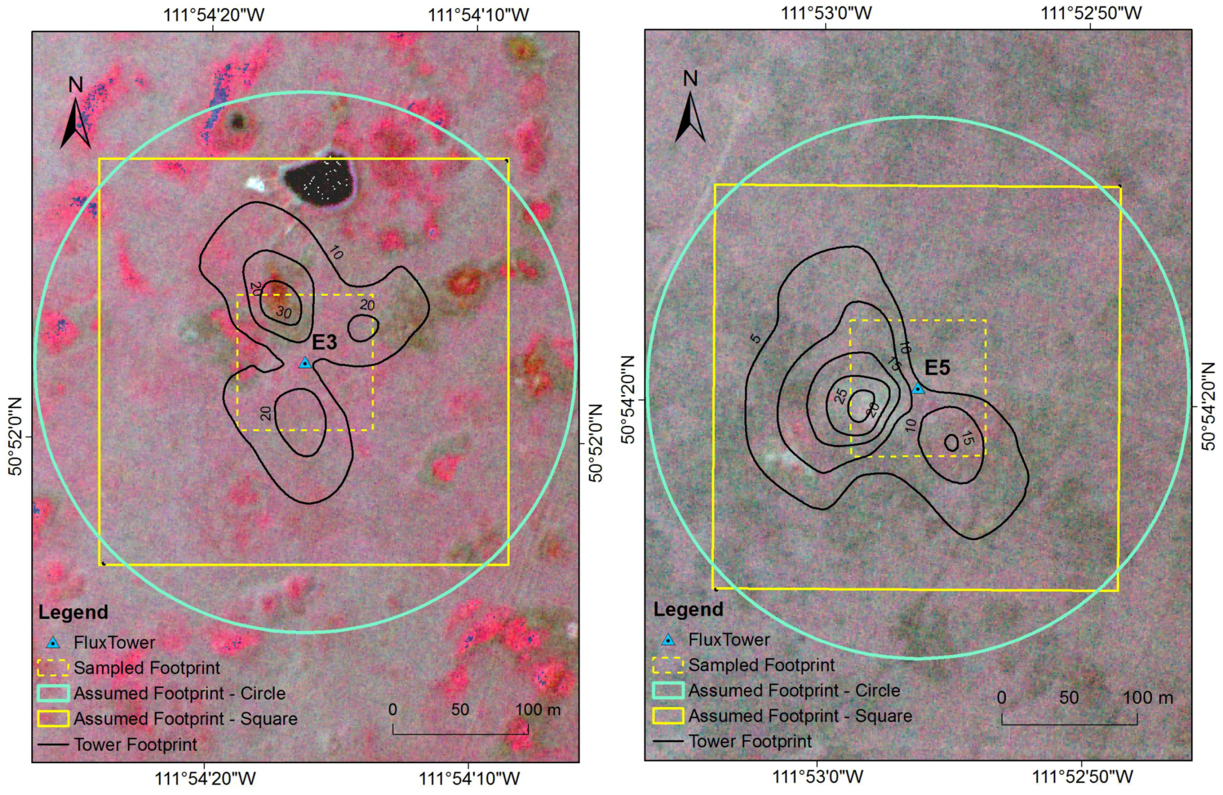
2.7. Sensitivity Analysis of Footprint
2.8. Vegetation Map Analysis
2.9. Biodiversity Estimation
3. Results
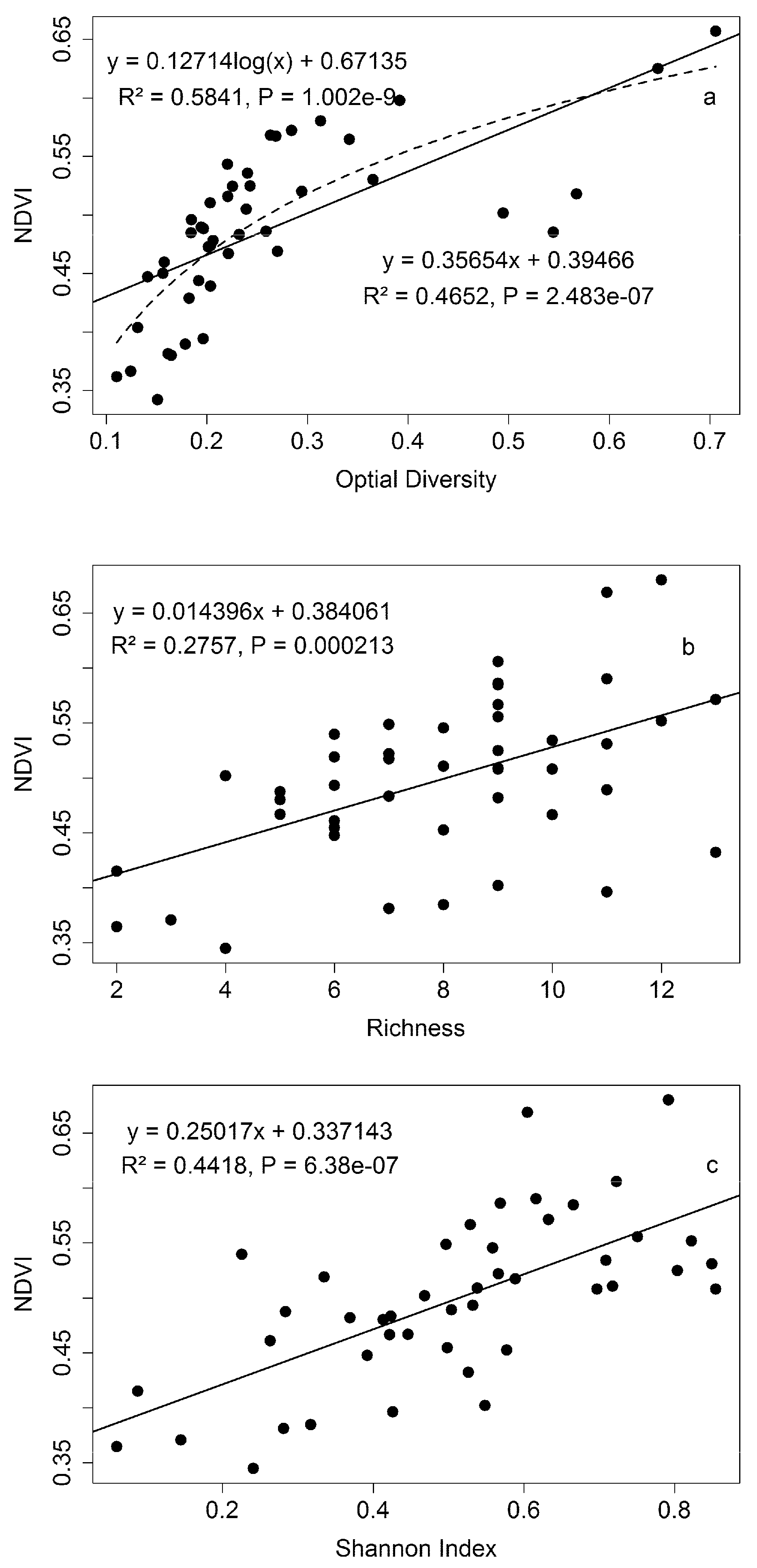
3.1. Model Results
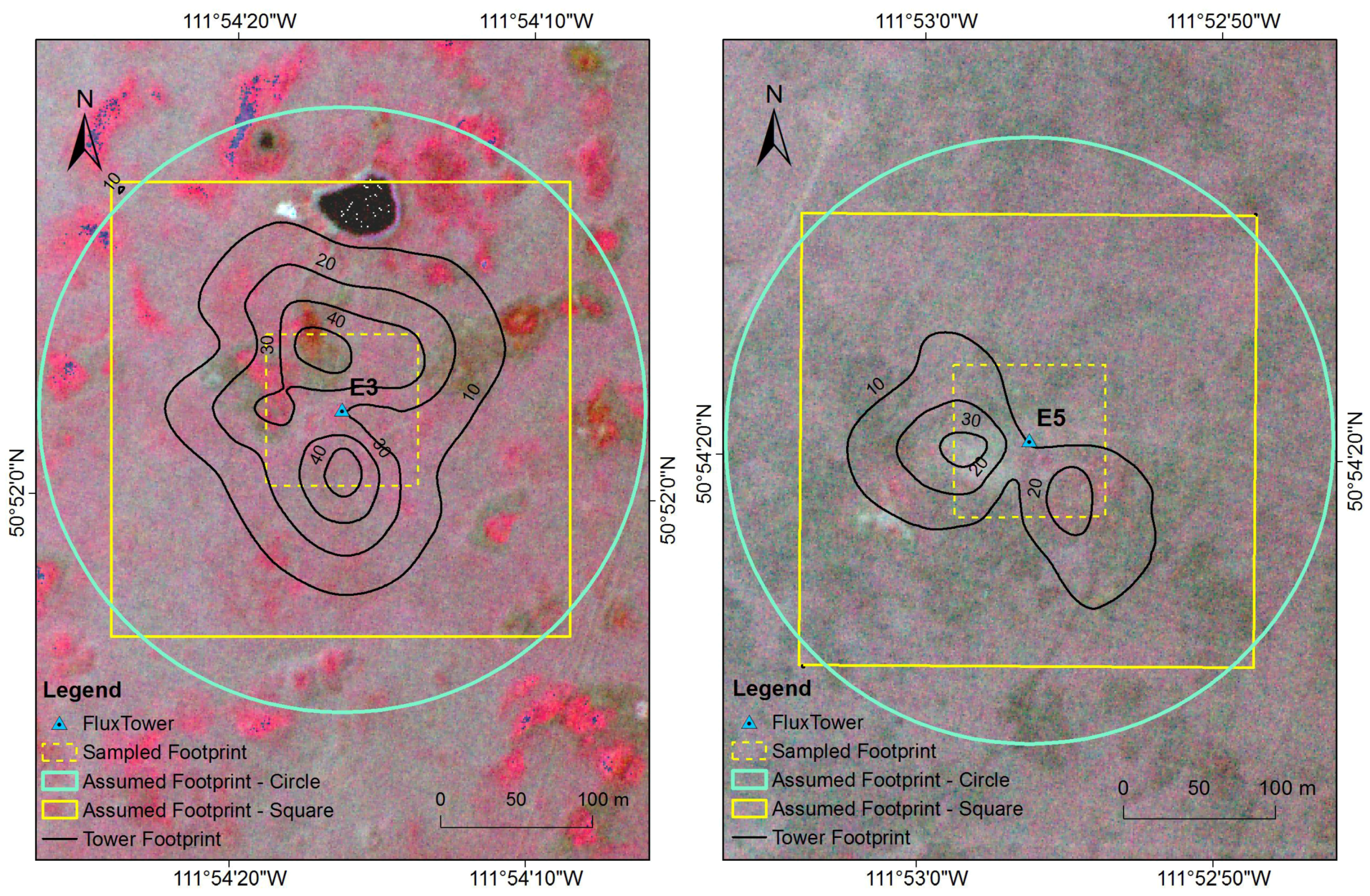
3.2. Sensitivity Analysis of Footprint
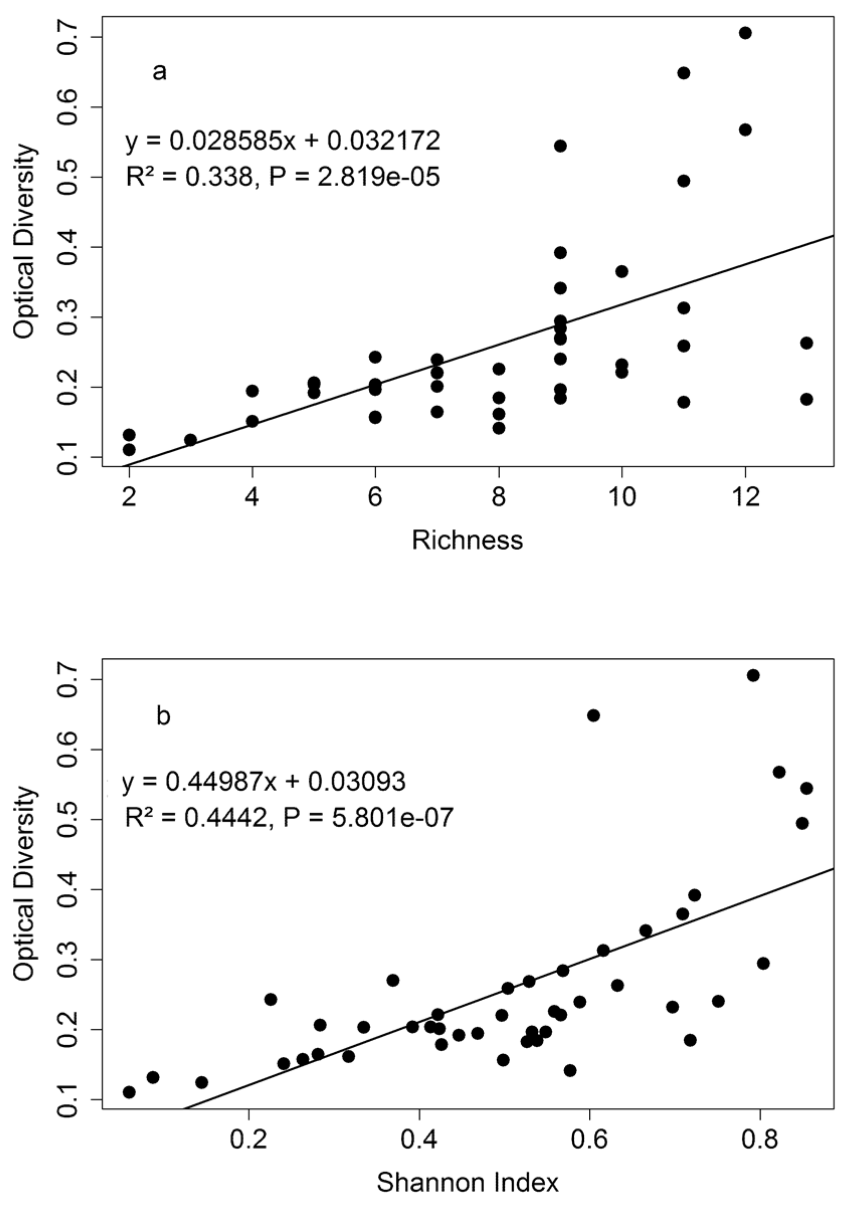
3.3. Diversity Estimation at Calibration Sites
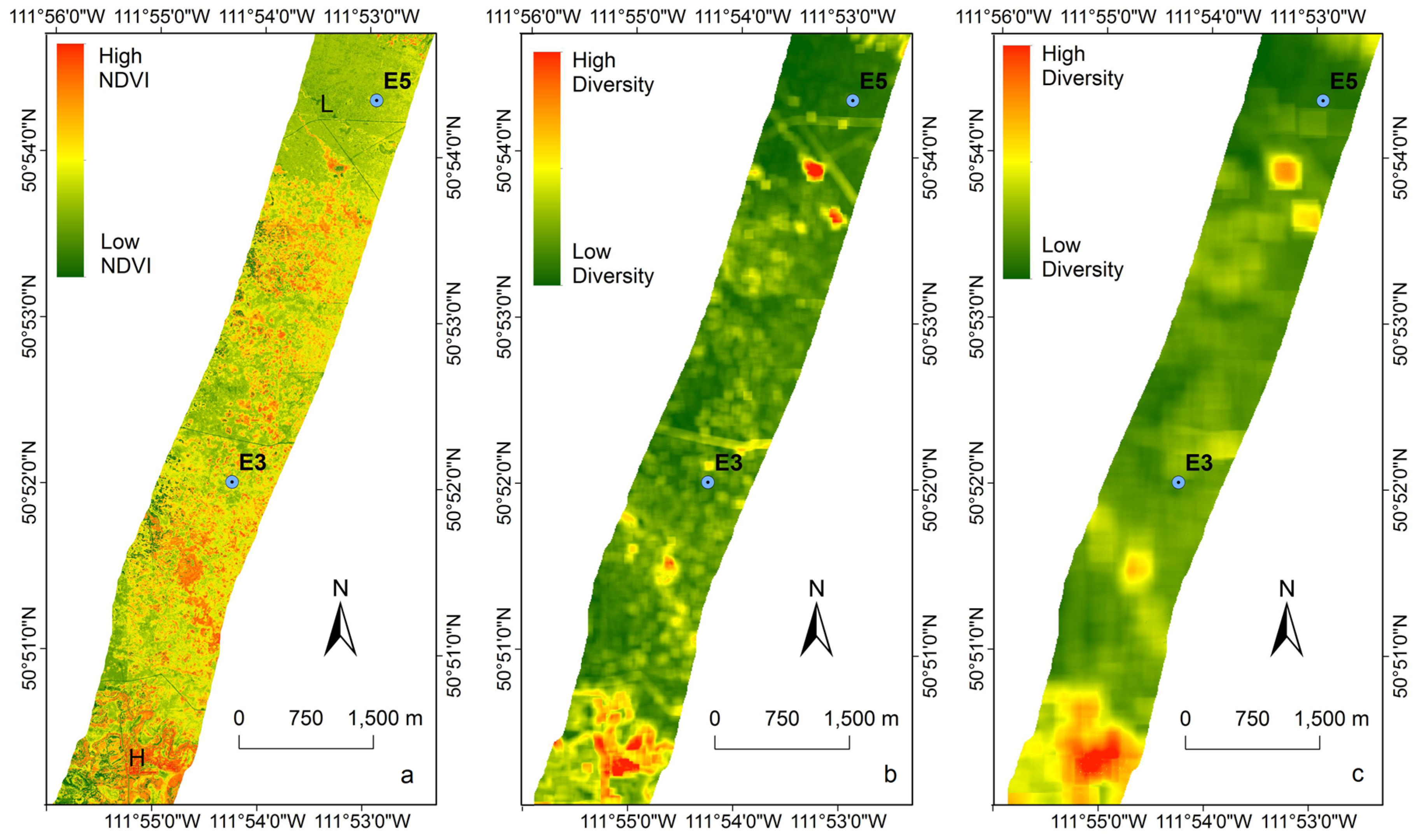
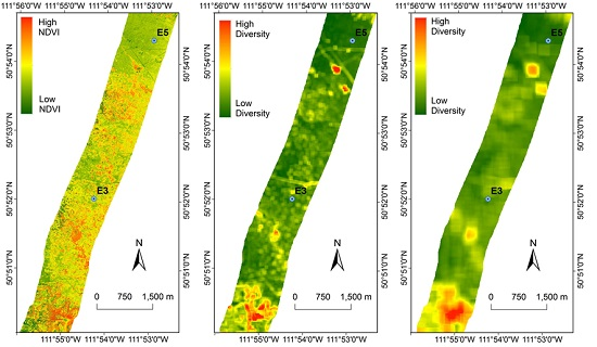
3.4. Extrapolating to a Larger Region
4. Discussion
4.1. Green Biomass and NDVI
4.2. Sensitivity Analysis of Footprint
4.3. Biodiversity—Ecosystem Function
5. Conclusions
Supplementary Materials
Acknowledgments
Author Contributions
Conflicts of Interest
References
- Sala, O.E.; Lauenroth, W.K.; McNaughton, S.J.; Rusch, G.; Zhang, X. Biodiversity and ecosystem functioning in grasslands. In Functional Roles of Biodiversity: A Global Perspective; Mooney, H.A., Cushman, J.H., Medina, E., Sala, O.E., Schulze, E.D., Eds.; John Wiley and Sons Ltd.: Chichester, UK, 1996; pp. 129–149. [Google Scholar]
- Hunt, E.R.; Everitt, J.H.; Ritchie, J.C.; Moran, M.S.; Booth, D.T.; Anderson, G.L.; Clark, P.E.; Seyfried, M.S. Applications and research using remote sensing for rangeland management. Photogramm. Eng. Remote Sens. 2003, 69, 675–693. [Google Scholar] [CrossRef]
- Sims, P.L.; Risser, P.G. Grasslands. In Northern American Terrestrial Vegetation; Barbour, M.G., Billings, W.D., Eds.; Cambridge University Press: Cambridge, UK, 2000; pp. 323–356. [Google Scholar]
- Adams, B.W.; Richman, J.; Poulin-Klein, L.; France, K.; Moisey, D.; Mcneil, R.L. Range Plant Communities and Range Health Assessment Guidelines for the Dry Mixedgrass Natural Subregion of Alberta; Rangeland Management Branch, PolicyDivision, Alberta Environment and Sustainable Resource Development: Lethbridge, AB, Canada, 2013. [Google Scholar]
- Bernhardt-Römermann, M.; Römermann, C.; Sperlich, S.; Schmidt, W. Explaining grassland biomass—The contribution of climate, species and functional diversity depends on fertilization and mowing frequency. J. Appl. Ecol. 2011, 48, 1088–1097. [Google Scholar] [CrossRef]
- Bork, E.W.; West, N.E.; Price, K.P.; Walker, J.W. Rangeland cover component quantification using broad (TM) and narrow-band (1.4 NM) spectrometry. J. Range Manag. 1999, 52, 249–257. [Google Scholar] [CrossRef]
- Booth, D.T.; Tueller, P.T. Rangeland monitoring using remote sensing. Arid Land Res. Manag. 2003, 17, 455–467. [Google Scholar] [CrossRef]
- Piñeiro, G.; Oesterheld, M.; Paruelo, J.M. Seasonal variation in aboveground production and radiation-use efficiency of temperate rangelands estimated through remote sensing. Ecosystems 2006, 9, 357–373. [Google Scholar] [CrossRef]
- Clark, D.A.; Brown, S.; Kicklighter, D.W.; Chambers, J.Q.; Thomlinson, J.R.; Ni, J. Measuring net primary production in forest: Concepts and field methods. Ecol. Appl. 2001, 11, 356–370. [Google Scholar] [CrossRef]
- Monteith, J.L. Solar radition and productivity in tropical ecosystems. J. Appl. Ecol. 1972, 9, 747–766. [Google Scholar] [CrossRef]
- Monteith, J.L.; Moss, C.J. Climate and the efficiency of crop production in Britain. Philos. Trans. Royal Soc. B 1977, 281, 277–294. [Google Scholar] [CrossRef]
- Yuan, W.; Liu, S.; Zhou, G.; Zhou, G.; Tieszen, L.L.; Baldocchi, D.; Bernhofer, C.; Gholz, H.; Goldstein, A.H.; Goulden, M.L.; et al. Deriving a light use efficiency model from eddy covariance flux data for predicting daily gross primary production across biomes. Agric. For. Meteorol. 2007, 143, 189–207. [Google Scholar] [CrossRef]
- Gitelson, A.A.; Gamon, J.A. The need for a common basis for defining light-use efficiency: Implications for productivity estimation. Remote Sens. Environ. 2015, 156, 196–201. [Google Scholar] [CrossRef]
- Gamon, J.A.; Field, C.B.; Roberts, D.A.; Ustin, S.L.; Valentini, R. Functional patterns in an annual grassland during an AVIRIS overflight. Remote Sens. Environ. 1993, 44, 239–253. [Google Scholar] [CrossRef]
- Flanagan, L.B.; Sharp, E.J.; Gamon, J.A. Application of the photosynthetic light-use efficiency model in a northern Great Plains grassland. Remote Sens. Environ. 2015, 168, 239–251. [Google Scholar] [CrossRef]
- Tucker, C.J.; Townshend, J.R.; Goff, T.E. African land-cover classification using satellite data. Science 1985, 227, 369–375. [Google Scholar] [CrossRef] [PubMed]
- DeFries, R.S.; Townshend, J.R.G. NDVI-derived land cover classifications at a global scale. Int. J. Remote Sens. 1994, 15, 3567–3586. [Google Scholar] [CrossRef]
- Hill, M.J. Vegetation index suites as indicators of vegetation state in grassland and savanna: An analysis with simulated SENTINEL 2 data for a North American transect. Remote Sens. Environ. 2013, 137, 94–111. [Google Scholar] [CrossRef]
- Gamon, J.A.; Field, C.B.; Goulden, M.L.; Griffin, K.L.; Hartley, A.E.; Joel, G.; Penuelas, J.; Valentini, R. Relationships between NDVI, canopy structure, and photosynthesis in three californian vegetation types. Ecol. Appl. 1995, 5, 28–41. [Google Scholar] [CrossRef]
- Pottier, J.; Malenovský, Z.; Psomas, A.; Homolová, L.; Schaepman, M.E.; Choler, P.; Thuiller, W.; Guisan, A.; Zimmermann, N.E. Modelling plant species distribution in alpine grasslands using airborne imaging spectroscopy Modellin. Biol. Lett. 2014, 10, 1–4. [Google Scholar] [CrossRef] [PubMed]
- Tilman, D.; Wedin, D.; Knops, J. Productivity and sustainability influenced by biodiversity in grassland ecosystems. Nature 1996, 379, 718–720. [Google Scholar] [CrossRef]
- Isbell, F.I.; Polley, H.W.; Wilsey, B.J. Biodiversity, productivity and the temporal stability of productivity: Patterns and processes. Ecol. Lett. 2009, 12, 443–451. [Google Scholar] [CrossRef] [PubMed]
- De Mazancourt, C.; Isbell, F.; Larocque, A.; Berendse, F.; De Luca, E.; Grace, J.B.; Haegeman, B.; Wayne Polley, H.; Roscher, C.; Schmid, B.; et al. Predicting ecosystem stability from community composition and biodiversity. Ecol. Lett. 2013, 16, 617–625. [Google Scholar] [CrossRef] [PubMed]
- Fraser, L.H.; Pither, J.; Jentsch, A.; Sternberg, M.; Zobel, M.; Askarizadeh, D.; Bartha, S.; Beierkuhnlein, C.; Bennett, J.A. Worldwide evidence of a unimodal relationship between productivity and plant species richness. Science 2015, 349, 302–306. [Google Scholar] [CrossRef] [PubMed]
- Connell, J.H. Diversity in tropical rain forests and coral reefs. Science 1978, 199, 1302–1310. [Google Scholar] [CrossRef] [PubMed]
- Grime, J.P. Competitive exclusion in herbaceous vegetation. Nature 1973, 242, 344–347. [Google Scholar] [CrossRef]
- Clark, M.L.; Roberts, D.A. Species-level differences in hyperspectral metrics among tropical rainforest trees as determined by a tree-based classifier. Remote Sens. 2012, 4, 1820–1855. [Google Scholar] [CrossRef]
- Xiao, Q.; Ustin, S.L.; McPherson, E.G. Using AVIRIS data and multiple-masking techniques to map urban forest tree species. Int. J. Remote Sens. 2004, 25, 5637–5654. [Google Scholar] [CrossRef]
- Clark, M.L.; Roberts, D.A.; Clark, D.B. Hyperspectral discrimination of tropical rain forest tree species at leaf to crown scales. Remote Sens. Environ. 2005, 96, 375–398. [Google Scholar] [CrossRef]
- Roberts, D.A.; Gardner, M.; Church, R.; Ustin, S.; Scheer, G. Mapping chaparral in the Santa Monica mountains using multiple endmember spectral mixture models. Remote Sens. Environ. 1998, 65, 267–279. [Google Scholar] [CrossRef]
- Lucas, R.; Bunting, P.; Paterson, M.; Chisholm, L. Classification of Australian forest communities using aerial photography, CASI and HyMap data. Remote Sens. Environ. 2008, 112, 2088–2103. [Google Scholar] [CrossRef]
- Palmer, M.W.; Earls, P.G.; Hoagland, B.W.; White, P.S.; Wohlgemuth, T. Quantitative tools for perfecting species lists. Environmetrics 2002, 13, 121–137. [Google Scholar] [CrossRef]
- Rocchini, D. Effects of spatial and spectral resolution in estimating ecosystem α-diversity by satellite imagery. Remote Sens. Environ. 2007, 111, 423–434. [Google Scholar]
- Rocchini, D.; Chiarucci, A.; Loiselle, S.A. Testing the spectral variation hypothesis by using satellite multispectral images. Acta Oecol. 2004, 26, 117–120. [Google Scholar] [CrossRef]
- Oldeland, J.; Wesuls, D.; Rocchini, D.; Schmidt, M.; Jürgens, N. Does using species abundance data improve estimates of species diversity from remotely sensed spectral heterogeneity? Ecol. Indic. 2010, 10, 390–396. [Google Scholar] [CrossRef]
- Rocchini, D.; Balkenhol, N.; Carter, G.A.; Foody, G.M.; Gillespie, T.W.; He, K.S.; Kark, S.; Levin, N.; Lucas, K.; Luoto, M.; et al. Remotely sensed spectral heterogeneity as a proxy of species diversity: Recent advances and open challenges. Ecol. Inform. 2010, 5, 318–329. [Google Scholar] [CrossRef]
- Féret, J.-B.; Asner, G.P. Mapping tropical forest canopy diversity using high-fidelity imaging spectroscopy. Ecol. Appl. 2014, 24, 1289–1296. [Google Scholar] [CrossRef]
- Boundary Files, 2011 Census, Catalogue no. 92-16-X. Statistics Canada, 2011.
- Becker, S. Mattheis Ranch Vegetation and Soil Inventory; Rangeland Research Institute, University of Alberta: Edmonton, AB, Canada, 2013. [Google Scholar]
- Gamon, J.A.; Coburn, C.; Flanagan, L.B.; Huemmrich, K.F.; Kiddle, C.; Sanchez-Azofeifa, G.A.; Thayer, D.R.; Vescovo, L.; Gianelle, D.; Sims, D.A.; et al. SpecNet revisited: Bridging flux and remote sensing communities. Can. J. Remote Sens. 2010, 36, S376–S390. [Google Scholar] [CrossRef]
- Huemmrich, K.F.; Black, T.A.; Jarvis, P.G.; McCaughey, J.H.; Hall, F.G. High temporal resolution NDVI phenology from micrometeorological radiation sensors. J. Geophys. Res. 1999, 104, 27935. [Google Scholar] [CrossRef]
- Gamon, J.A.; Cheng, Y.; Claudio, H.; MacKinney, L.; Sims, D.A. A mobile tram system for systematic sampling of ecosystem optical properties. Remote Sens. Environ. 2006, 103, 246–254. [Google Scholar] [CrossRef]
- Conel, J.E.; Green, R.O.; Vane, G.; Bruegge, C.J.; Alley, R.E.; Curtiss, B.J. AIS-2 radiometry and a comparison of methods for the recovery of ground reflectance. In Proceedings of the 3rd Airborne Imaging Spectrometer Data Analysis Workshop; Vane, G., Ed.; Jet Propulsion Laboratory: Pasadena, CA, USA, 1987; pp. 18–47. [Google Scholar]
- Damm, A.; Erler, A.; Hillen, W.; Meroni, M.; Schaepman, M.E.; Verhoef, W.; Rascher, U. Modeling the impact of spectral sensor configurations on the FLD retrieval accuracy of sun-induced chlorophyll fluorescence. Remote Sens. Environ. 2011, 115, 1882–1892. [Google Scholar] [CrossRef]
- Kljun, N.; Calanca, P.; Rotach, M.W.; Schmid, H.P. A simple parameterisation for flux footprint predictions. Bound. Layer Meteorol. 2004, 112, 503–523. [Google Scholar] [CrossRef]
- Garratt, J.R. The internal boundary layer—A Review. Bound. Layer Meteorol. 1990, 50, 171–203. [Google Scholar] [CrossRef]
- Leclerc, M.Y.; Thurtell, G.W. Footprint prediction of scalar fluxes using a markovian analysis. Bound. Layer Meteorol. 1990, 52, 247–258. [Google Scholar] [CrossRef]
- Shannon, C.E. A mathematical theory of communication. Bell Syst. Tech. J. 1948, 27, 379–423, 623–656. [Google Scholar] [CrossRef]
- Wehlage, D.C. Monitoring Year-to-Year Variability in Dry Mixed-Grass Prairie Yield Using Multi-Sensor Remote Sensing. Master’s Thesis, University of Alberta, Edmonton, AB, Canada, 2012. [Google Scholar]
- Schmid, H.P. Footprint modeling for vegetation atmosphere exchange studies: A review and perspective. Agric. For. Meteorol. 2002, 113, 159–183. [Google Scholar] [CrossRef]
- Tilman, D. The influence of functional diversity and composition on ecosystem processes. Science 1997, 277, 1300–1302. [Google Scholar] [CrossRef]
- Sala, O.E.; Chapin, F.S.; Armesto, J.J.; Berlow, E.; Bloomfield, J.; Dirzo, R.; Huber-Sanwald, E.; Huenneke, L.F.; Jackson, R.B.; Kinzig, A.; et al. Global biodiversity scenarios for the year 2100. Science 2000, 287, 1770–1774. [Google Scholar] [CrossRef] [PubMed]
- Isbell, F.; Calcagno, V.; Hector, A.; Connolly, J.; Harpole, W.S.; Reich, P.B.; Scherer-lorenzen, M.; Schmid, B.; Tilman, D.; Van Ruijven, J.; et al. High plant diversity is needed to maintain ecosystem services. Nature 2011, 477, 199–202. [Google Scholar] [CrossRef] [PubMed]
- Bork, E.W.; Irving, B.D. Seasonal availability of cool- and warm-season herbage in the northern mixed prairie. Rangelands 2015, 37, 178–185. [Google Scholar] [CrossRef]
- Wang, R.; Gamon, J.; Montgomery, R.; Townsend, P.; Zygielbaum, A.; Bitan, K.; Tilman, D.; Cavender-Bares, J. Seasonal variation in the NDVI–species richness relationship in a prairie grassland experiment (Cedar Creek). Remote Sens. 2016, 8, 128. [Google Scholar] [CrossRef]
- Gamon, J.A. Tropical sensing—Opportunities and challenges. In Hyperspectral Remote Sensing of Tropical and Subtropical Forests; Kalacska, M., Sanchez-Azofeifa, G.A., Eds.; CRC Press, Taylor & Francis Group: Boca Raton, FL, USA, 2008; pp. 297–304. [Google Scholar]
- Ustin, S.L.; Gamon, J.A. Remote sensing of plant functional types. New Phytol. 2010, 186, 795–816. [Google Scholar] [CrossRef] [PubMed]
- Magurran, A.E. Measuring Biological Diversity; Blackwell Publishing: Malden, MA, USA, 2004. [Google Scholar]
- Nijs, I.; Roy, J. How important are species richness, species evenness and interspecific differences to productivity? A mathematical model. Oikos 2000, 88, 57–66. [Google Scholar] [CrossRef]
- Wilsey, B.J.; Potvin, C. Biodiversity and ecosystem functioning: Importance of species evenness in an old field. Ecology 2000, 81, 887–892. [Google Scholar] [CrossRef]
- Kirwan, L.; Lüscher, A.; Sebastià, M.T.; Finn, J.A.; Collins, R.P.; Porqueddu, C.; Helgadottir, A.; Baadshaug, O.H.; Brophy, C.; Coran, C.; et al. Evenness drives consistent diversity effects in intensive grassland systems across 28 European sites. J. Ecol. 2007, 95, 530–539. [Google Scholar] [CrossRef]


| R2 | |
|---|---|
| NEE = −0.0226 × proxy NDVI + 1.3899 | 0.7701 |
| Green biomass = 409.82 × NDVI − 80.57 | 0.8246 |
| E3 | E5 | |
|---|---|---|
| 1 hectare square | 0.4931 | 0.3715 |
| 200 meter circle | 0.4746 | 0.3823 |
| 300 m × 300 m Square | 0.4668 | 0.3812 |
| Midday (5 h) | 0.4714 | 0.3745 |
| Monthly | 0.4732 | 0.3771 |
| Site | Richness (Vegetation Map) | Shannon Index (Vegetation Map) | Species Richness (Field Sampling) |
|---|---|---|---|
| E3 | 9 | 0.9060 | 26 |
| E5 | 3 | 0.1547 | 20 |
© 2016 by the authors; licensee MDPI, Basel, Switzerland. This article is an open access article distributed under the terms and conditions of the Creative Commons by Attribution (CC-BY) license (http://creativecommons.org/licenses/by/4.0/).
Share and Cite
Wang, R.; Gamon, J.A.; Emmerton, C.A.; Li, H.; Nestola, E.; Pastorello, G.Z.; Menzer, O. Integrated Analysis of Productivity and Biodiversity in a Southern Alberta Prairie. Remote Sens. 2016, 8, 214. https://doi.org/10.3390/rs8030214
Wang R, Gamon JA, Emmerton CA, Li H, Nestola E, Pastorello GZ, Menzer O. Integrated Analysis of Productivity and Biodiversity in a Southern Alberta Prairie. Remote Sensing. 2016; 8(3):214. https://doi.org/10.3390/rs8030214
Chicago/Turabian StyleWang, Ran, John A. Gamon, Craig A. Emmerton, Haitao Li, Enrica Nestola, Gilberto Z. Pastorello, and Olaf Menzer. 2016. "Integrated Analysis of Productivity and Biodiversity in a Southern Alberta Prairie" Remote Sensing 8, no. 3: 214. https://doi.org/10.3390/rs8030214
APA StyleWang, R., Gamon, J. A., Emmerton, C. A., Li, H., Nestola, E., Pastorello, G. Z., & Menzer, O. (2016). Integrated Analysis of Productivity and Biodiversity in a Southern Alberta Prairie. Remote Sensing, 8(3), 214. https://doi.org/10.3390/rs8030214