Tree Species Abundance Predictions in a Tropical Agricultural Landscape with a Supervised Classification Model and Imbalanced Data

Abstract

Mapping species through classification of imaging spectroscopy data is facilitating research to understand tree species distributions at increasingly greater spatial scales. Classification requires a dataset of field observations matched to the image, which will often reflect natural species distributions, resulting in an imbalanced dataset with many samples for common species and few samples for less common species. Despite the high prevalence of imbalanced datasets in multiclass species predictions, the effect on species prediction accuracy and landscape species abundance has not yet been quantified. First, we trained and assessed the accuracy of a support vector machine (SVM) model with a highly imbalanced dataset of 20 tropical species and one mixed-species class of 24 species identified in a hyperspectral image mosaic (350–2500 nm) of Panamanian farmland and secondary forest fragments. The model, with an overall accuracy of 62% ± 2.3% and F-score of 59% ± 2.7%, was applied to the full image mosaic (23,000 ha at a 2-m resolution) to produce a species prediction map, which suggested that this tropical agricultural landscape is more diverse than what has been presented in field-based studies. Second, we quantified the effect of class imbalance on model accuracy. Model assessment showed a trend where species with more samples were consistently over predicted while species with fewer samples were under predicted. Standardizing sample size reduced model accuracy, but also reduced the level of species over- and under-prediction. This study advances operational species mapping of diverse tropical landscapes by detailing the effect of imbalanced data on classification accuracy and providing estimates of tree species abundance in an agricultural landscape. Species maps using data and methods presented here can be used in landscape analyses of species distributions to understand human or environmental effects, in addition to focusing conservation efforts in areas with high tree cover and diversity.

1. Introduction

Mapping tree species distributions in tropical landscapes has been a clear goal of the remote sensing community [1,2] because of its ecological applications for understanding spatial patterns of tree populations and species co-occurrence [3,4], and conservation applications to identify regions of high diversity [5], invasive species [6,7,8], or rare and ecologically important species [9]. High spatial resolution imaging spectroscopy that can resolve individual tree crowns and capture small differences in reflectance patterns among species can help achieve these goals [10].

To achieve these application goals, species classifications are moving beyond understanding the spectral separability of species and towards operational species mapping, where classification models are applied to an entire remotely sensed image to predict species identity and locations across a landscape [3,11,12,13]. Important components to the success of operational species mapping are the characteristics of the input, or training data, including the spectral uniqueness of each species, the number of species, and the sample size of each species.

A particular challenge for operational species mapping in tropical forest ecosystems is the high species diversity, which requires uniquely identifying many species, most of which have few individuals on the landscape and are thus hard to include with sufficient sample size in training data sets. Many studies have explored the effect of the spectral uniqueness of species at multiple scales on the success of classification models [9,14,15]. These studies highlight the contributions of crown structure, phenology, and leaf chemistry of a species’ unique spectral signature to spectral separability. Other studies have explored the scope of the model, quantifying the decline in prediction accuracy with an increase in the number of classes [16] and smaller class sample sizes [17], in addition to providing guidelines for the optimal sample size needed to achieve maximum accuracy given the number of classes in the model [15].

However, the optimal sample size is difficult to achieve in tropical forests given the low and widely variable density of each species across the landscape. Even in the most diverse forests, some species are relatively common [18], but most are very rare, leading to high unevenss of individuals across species. Agricultural landscapes also have uneven speciesdistributions because farmers selectively leave species that they find desirable [19,20]. Sampling the natural abundance of species will lead to highly skewed sample size across classes, but increasing the sample size of rare species can be time-consuming and costly.

Despite the recognition that variation in the sample size across classes may influence model errors [21], direct quantification of these errors in remote sensing applications has received little attention. To isolate the effects of changes in the number of species and sample sizes, studies have standardized the sample size for each species, giving species equal weight in the model [15,16,17]. In reality, equal sample size across all species is generated by either time-consuming field efforts to generate a large dataset of the rare species, or by subsampling the data from the large classes, which with random sample selection, may result in the removal of potentially useful data points for classifying the common species. Therefore, there is a need to test classification models with field datasets that are typically generated in these types of landscapes.

Tree species classification models often use a set of labeled data points generated by directly matching individual trees identified in the field with pixels in a remotely sensed image, with supervised methods requiring laballed data for all species of interest. The ideal labeled dataset for supervised species classification models should span the spatial extent of the image to capture the full variation in species’ spectra [22], and include many crowns of all species, acknowledging that the exact number is highly dependent on the spectral uniqueness of all species [15]. Field datasets will often reflect the landscape distribution of species abundances, where the sample sizes may be small and uneven across all species. For example, studies that apply supervised species classification models to imaging spectroscopy data of forested landscapes show an imbalance across species sample sizes, often dominated by one or two classes each composing 30% of the labeled or training data (

Table 1. Summary of species classifications using imaging spectroscopy to classify 3 or more species in temperate and tropical forests. Studies using spectral mixture analysis were not included. Imbalance is calculated as the exponential decay of a species rank abundance curve with the sample size for each class/species. The intercept (I) represents the relative abundance of the largest class and the power (P) represents the degree of imbalance (See Figure S1).

Study	Sensor, Location	Spatial Resolution	Spectral Resolution	Number of Species	Imbalance	Accuracy (Classification Method)
Clark, Roberts, and Clark 2005 [9]	La Selva, Costa Rica; HYDICE	1.6 m	VIS-SWIR (400–2500 nm; reduced to 30 bands selected)	7	I = 37 P = −0.956	OA = 92% (LDA)
Jones et al. 2010 [27]	Gulf Islands, British Columbia; AISA Dual	2 m	VIS-SWIR (429–2400 nm, reduced to 40 spectral bands)	11	I = 31 P = −0.896	OA = 72% (SVM)
Dalponte et al. 2012 [23]	Val di Sella, Italy; AISA Eagle	1 m	VIS-NIR (400–990 nm; 126 bands)	7 species + 1 non-forest class	I = 35 P = −0.990	OA = 74% (SVM)
Cho et al. 2012 [24]	Kruger National Park (KNP), South Africa; CAO Alpha	1.1 m	VIS-NIR (384–1054 nm; 72 bands)	6	I = 31 P = −0.637	OA = 65% (ML)
Clark and Roberts 2012 [28]	La Selva, Costa Rica; HYDICE	1.6 m	VIS-SWIR (400–2500 nm; 210 bands)	Same as Clark et al. 2005	Same as Clark et al. 2005	OA = 87% (RF)
Colgan et al. 2012 [29]	KNP, South Africa; CAO Alpha	1.1 m	VIS-NIR (385–1054 nm; 72 bands)	15 species + 1 mixed species class	I = 15 P = −0.494	OA = 76% (RBF-SVM)
Feret and Asner 2012 [16]	Hawaii, USA; CAO Alpha	0.56 m	VIS-NIR (390–1044 nm; 24 bands)	17 *	I = 25 P = −0.821	OA = 73% (RBF-SVM)
Feret and Asner 2012 [13]	Hawaii, USA; CAO Alpha	0.56 m	VIS-NIR (390–1044 nm; 24 bands)	9*	I = 39 P = −1.161	Balanced accuracy = 66% (SVM)
Alonzo et al. 2013 [17]	Santa Barbara, CA; AVIRIS	3 m	VIS-SWIR (365–2500 nm, 178 bands)	15	Not applicable	OA = 86% (CDA, LDA)
Baldeck and Anser 2015 [11]	BCI, Panama; CAO AToMS	2 m	VIS-SWIR (380–2512 nm)	3	Not applicable	Recall = 94-97% Prec. = 94-100% (Single-class SVM)
This study	Azuero Peninsula, Panama; CAO AToMS	2 m	VIS-SWIR (380–2512 nm)	20 + 1 mixed species class	I = 20 P = −0.756	OA = 63% (RBF-SVM)

Note：The accuracies listed are specific to species classifications with spectral data only when these results were available. * indicates that 50 pixels were used in the classification model. CDA = Canonical Descriminant Analysis; I = Intercept; LDA = Linear Discriminant Analysis; ML = Maximum Likelihood; OA = Overall accuracy; P = Power; RF = Random Forests; SVM = Support Vector Machine.

, Figure S1). Furthermore, a few studies discuss the potential impact of imbalance on their study results, though they do not quantify the effect directly [23,24,25,26]. This shows there is awareness that imbalanced predictions due to sample size are important for the interpretation of results, but it has yet to be directly measured in multi-species classification studies.

The Support Vector Machine (SVM) algorithm has been widely utilized for the purpose of species classification because of its ability to produce relatively accurate predictions, even with limited training data [16,30,31,32]. However, training an SVM model using a data set with uneven class sizes is problematic because when presented with imbalanced data, the algorithm may favor the larger classes, resulting in a classification preference towards such classes. While these effects of imbalance have been highlighted in many two-class applications of SVM [33,34,35], to our knowledge there have been no previous quantitative assessments of this phenomenon in remote sensing applications, particularly in the context of multiclass species classifications. In the case of multiclass species classification, misclassifications may not be solely due to the spectral similarity of species, but also due to poor model optimization from uneven class sizes. For tree species classification applications, the class imbalance problem translates to unequal penalties in the misclassification of common and rare tree species. When applying the classification model to the entire landscape, this preference for large classes influences the predictions of species diversity and distribution patterns, such as the abundance or scarcity of certain species [36].

This paper provides landscape predictions of tree species in a tropical agricultural landscape of Panama and analyzes the effect of imbalanced data on prediction accuracy and landscape species abundance predictions. We compare how remote sensing-derived landscape predictions of species abundance compare to field inventories of species abundance. To assess the importance of imbalanced data in a landscape species prediction, we quantified the effect of widely differing training class sizes in a 21-species class model with imaging spectroscopy data. We measured the difference in model performance when implementing two strategies for reducing the effect of imbalance; eliminating imbalance by standardizing class sizes, and adjusting model predictions by including information on class size into the classification model. The ultimate application of this work is quantifying the landscape species composition and understanding the contribution of common and rare tree species in an area with little intact forest. Understanding species distributions on tropical agricultural landscapes are important for numerous reasons, including understanding how these landscapes may develop if allowed to develop secondary forest [37].

2. Materials and Methods

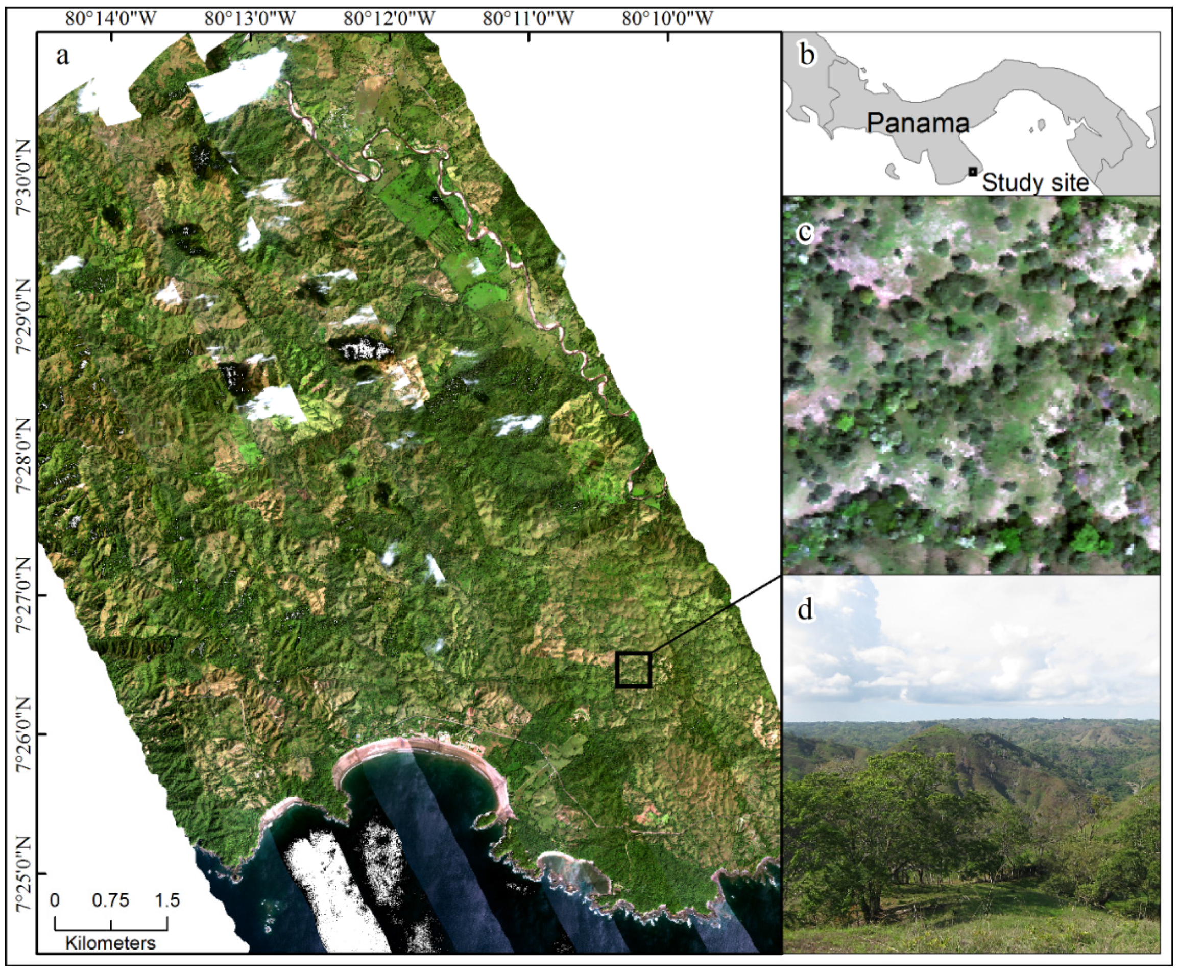
2.1. Study Site

Our region of focus was the 8000 km² Azuero Peninsula of Panama located at approximately 7.5° N and 80.5° W (Figure 1). The Azuero landscape is dominated by agricultural fields and pastures with little forest cover, a result of its long history of forest clearing for cattle and farming initiated by Spanish colonists that intensified during the second half of the 20th Century. Though now dominated by agricultural land use, the historical ecoregion coverage of the peninsula was tropical dry broadleaf forest to the south and east, and moist broadleaf forest in the west [38]. In the most southern region of the peninsula where this study was conducted, mean annual rainfall is 1946 ± 65 mm·yr⁻¹ with 4.1 drought months characterized by less than 100 mm of rainfall per month. The study site for this research is dominated by active and abandoned cattle pastures on hilly terrain, narrow riparian forests, and small secondary forest fragments [20]. The analysis presented here is part of a larger project to quantify the species diversity and aboveground biomass of trees in agricultural landscapes. Therefore the analysis included only trees within pastures, along live fences, or on the edges of small forest patches rather than trees in closed canopy forest.

2.2. Airborne and Field Data Collection

In January 2012, members of the Carnegie Airborne Observatory (CAO) imaged 22,857 ha of the southern Azuero Peninsula using the Airborne Taxonomic Mapping Systems (AToMS) sensor package (Figure 1a). AToMS collects imaging spectrometer data (380–2510 nm; 5 nm bandwidth) at a spatial resolution of 2 m. The data were downsampled from 5 to 10 nm resolution to reduce data volume and increase the signal-to-noise [39]. A bidirectional reflectance distribution correction model was applied to the image mosaic to reduce flight line artifacts [29]. Additionally, dual laser waveform light detection and ranging (lidar) data were collected at a resolution of 1.12 m. Ground and canopy digital elevation models were estimated from the point-cloud lidar data (see [39,40] for methodological details).

The canopy model was not used to develop the classification algorithm, but was segmented to produce an image-wide layer of individual tree crowns on which the classification algorithm was applied. We selected pixels with the strongest live vegetation signal by removing shaded pixels with near-infrared (NIR; 860 nm) reflectance less than 30% and low leaf density pixels with values in the Normalized Difference Vegetation Index (NDVI) less than 0.5 [29].

In May–July of 2012 and 2013, 1140 individual tree crowns of 76 species were mapped in the field and identified to species with the help of botanists. Lack of road access and hilly terrain restricted field mapping to locations accessible in a day’s walk or horse ride from the nearest road (3 km maximum). Trees on private lands were visited, with permission from the landowners, and marked in high-resolution (1.12 m) georeferenced images derived from the CAO lidar using a tablet computer equipped with a GPS (Xplore Technologies; Austin, TX). Later, exact tree crown boundaries were digitized on the 2 m CAO spectral image, using ENVI 4.8 (Exelis Visual Information Solutions, Boulder, CO, USA).

A total of 1112 crowns from 44 species were used to train and test the classification model (

Table 2. Summary of field data. Twenty-one classes were used to train the SVM model. The class proportions were calculated as the number of pixels for the class divided by the total number of pixels.

Species Code	Species	Family	Crowns	Pixels	Class Proportion
ANACEX	Anacardium excelsum	Anacardiaceae	31	672	0.023
ANDIIN	Andira inermis	Fabaceae	24	618	0.025
BYRSCR	Byrsonima crassifolia	Malpighiaceae	29	402	0.014
CALYCA	Calycophyllum candidissimum	Rubiaceae	60	1163	0.040
CEDROD	Cedrela odorata	Meliaceae	83	1960	0.070
COCCCA	Coccoloba caracasana	Polygonaceae	24	422	0.014
CORDAL	Cordia alliodora	Boraginaceae	31	436	0.017
DIPHAM	Diphysa americana	Fabaceae	53	781	0.029
ENTECY	Enterolobium cyclocarpum	Fabaceae	82	4565	0.173
GENIAM	Genipa americana	Rubiaceae	24	315	0.013
GUAZUL	Guazuma ulmifolia	Malvaceae	116	2902	0.104
HURACR	Hura crepitans	Euphorbiaceae	62	2154	0.083
LUEHSE	Luehea seemannii	Malvaceae	21	510	0.020
PLA1PI	Platymiscium pinnatum	Fabaceae	47	1441	0.053
POCHQU	Pachira quinata	Bombacaceae	27	382	0.016
SAPIGL	Sapium glandulosum	Euphorbiaceae	24	416	0.018
SCIAEX	Sciadodendron excelsum	Araliaceae	20	131	0.004
SPONMO	Spondias mombin	Anacardiaceae	73	1651	0.064
STERAP	Sterculia apetala	Malvaceae	21	689	0.025
TAB1RO	Tabebuia rosea	Bignoniaceae	38	624	0.025
OTHERS	24 species		222	4822	0.172
Total			1112	27,056

). The field dataset used to train the model exhibited moderate imbalance relative to other species classification models, with the maximum class representing 19% (Table 1, Figure S1). All species with fewer than three individual crowns were excluded, eliminating 32 species from the field dataset of the original 76 species. The three-crown threshold was selected because at least three crowns were needed to perform a three-fold cross-validation of the classification, in which the field dataset was divided into three groups; two for training, and one for testing.

Only the 20 species with 20 crowns or more were analyzed as single-species classes. A large increase in overall model accuracy was seen when including only species with more than 20 crowns (Figure S2) and is similar to thresholds in crown numbers used in other studies [15]. All crowns of the 24 species with fewer than 20 crowns were grouped together into a mixed species class called “Others”.

2.3. Training of an SVM Classifier

We used SVM classifier due to its ability to handle high dimensional data with small class sample sizes. To utilize SVM for the purpose of multiclass classification, the one-against-one approach was adopted, where binary classifications were made for each pair of classes (total of 210 models). Test spectra were assessed and assigned a potential class by each model. Final classification decision for test spectra were made across all 210 comparisons using the majority vote. We used the “e1071” package [41], which is an implementation of SVM, in the R statistical program [42].

Parameter Optimization for an SVM Model

During the model training, the SVM algorithm identifies a subset of the training data, called support vectors, that uniquely define a decision hyperplane that separates the two classes. In the original (hard) SVM algorithm [43], support vectors are chosen to maximize the margin, the distance between any support vector and the decision plane, while not allowing for any of the training data points to fall on the wrong side of the decision hyperplane or within the margin. For real-world data, complete separation is most likely not feasible or even desirable. Unlike hard SVM, soft SVM allows some of the training points to fall on the wrong side of the decision hyperplane or within the margin in order to favor a larger margin. Allowing a larger margin contributes to the robustness of SVM against noise and outliers in the training data in cases where such data do not affect the decision hyperplane strongly. The tradeoff between the margin and the adherence to the training data is controlled by the cost parameter, C, which has to be input to the SVM algorithm. With imbalanced data, the discrepancies in sample size among classes also affects this tradeoff. A larger training class has a smaller portion of its data points falling on the wrong side of the hyperplane relative to a smaller class. Therefore, the hyperplane may be shifted towards the smaller class ([44], Figure 2).

Furthermore, nonlinear SVM is often needed. Usually a nonlinear transformation of complex data into a higher dimensional space improves class separability [30,45]. This nonlinear transformation has been embedded in kernel SVM by redefining the similarity of two spectra xi and xj using a kernel function k, instead of defending their similarity as linear SVM does, namely xi·xj , the dot product of the two spectra. We utilized the RBF kernel, which is a popular choice for the problem of image classification [30,45], and is defined as:

k(xi, xj): = exp(− || xi − xj ||2/ γ2)

(1)

where γ is the width parameter.

In summary, to have the right balance between the robustness and faithfulness to the training data and to accommodate the complexity of hyperspectral data using nonlinearly, two parameters must be supplied to the SVM: the width parameter γ and the cost parameter C. For our study, a pair of parameter values (C, γ) that optimized the model performance on a validation set was chosen by a grid search of possible parameters values, a traditional way of parameter optimization.

2.4. Assessment of SVM Classifier

To assess the performance of the SVM classification models, we measured how well the model predicted the species of the test data. Therefore, labeled data were split into the training and test sets. In order to avoid performance bias due to an arbitrary split of the labeled data, we resplit the labeled data into the training and the test sets for a total of 30 splits and averaged the models performance. This repeated cross-valdiation approach [46] has been used in similar studies to estimate the sensivity and average accuracy of the model using different training and test data [15,17,24,26,29]. We used a three-fold design where the labeled dataset was split into three groups of crowns where two groups were used to train the model and one group was reserved to test the model. Within this split of the data, three iterations were performed where all crown groups were used for both training and testing (at different iterations). The grouping of individual crowns into three groups was repeated 10 times, therefore performing a total of 30 runs of the classification algorithm and obtaining 30 assessments of the algorithm. Cost and width parameters were optimized for each of the 30 iterations as described above.

While the model was run on pixel-level reflectance, classification performance was assessed on crowns different from those used for model training [15]. We scaled from pixel-level predictions to crown-level decisions using the majority vote among pixels of a crown where each crown was assigned to the species that had the most pixels predicted as that species [28] as a simple strategy to incorporate spatial information.

Measures of Classification Performance

Model performance of species classifications is commonly reported in terms of overall accuracy, calculated as the total number of pixels or crowns classified correctly out of all of the pixels or crowns in the test data. However, this metric is not appropriate for evaluating accuracy of imbalanced data because the accuracy can be overwhelmed by majority classes [33]. Precision and recall are informative metrics for multiclass models, especially those with imbalanced data [33,47]. Precision is a measure of exactness, or the number of class predictions that are truly of that class. It is calculated as the number of true observations of a class (true positives) divided by the number of predicted observations (sum of true positives and false positives). Precision is equivalent to user accuracy, a common metric reported in remote sensing classification applications [47,48]. Recall is a measure of completeness, or how well a class is detected. It is calculated as the number of true observations of a class divided by the number of true individuals of that class. Recall is equivalent to producer accuracy. Precision and recall can also be communicated in terms of error, as either errors of commission (1-user accuracy/precision) or errors of omission (1-producer accuracy/recall/sensitivity).

For a given class, differences in precision and recall accuracy indicate if the species is more or less abundant in test data predictions relative to its true abundance. We report the difference between these metrics as a prediction bias, calculated as recall minus precision. We use the general term of bias here to refer to a systematic error in predictions based on the relative occurrence of commission and omission errors. Negative values indicate a species with high precision relative to recall (alternatively low commission error and high omission error), meaning the model was careful when predicting the species, but in doing so, there were many individuals of that species that were not predicted. Ultimately, the species is underpredicted, or had fewer individuals of that species than exist in reality. Positive bias values indicate a species with low precision relative to recall (high commission error and low omission error), meaning the model was able to include all of the individuals that belonged to that species, but it also included individuals of other classes. Ultimately, the species is overpredicted, or included more individuals of that species than exist in reality. Prediction bias values near zero are optimal and show a balance between precision and recall, regardless of the magnitude of accuracy or error. Evaluating the relative magnitude of precision and recall for a given class is useful when the application of the classification is to determine relative abundances of species.

Another common metric to evaluate class predictions with imbalanced data is the F-score, which is the harmonic mean of precision and recall [33,47]. We calculated:

$$F-score=2·\left(\frac{precison · recall}{precision + recall}\right)$$

(2)

F-score increases with greater precision and recall and/or greater similarity between precision and recall. While the F-score does indicate the similarity of precision and recall measurements (more similar means a higher F-score), it does not indicate which metric is larger or smaller. For species-level measurements, we averaged each species F-score across all iterations. For model-level measurements, we treated all classes equally and calculated the macro-average of the F-score across all species and all iterations [47].

To quantify the effect of species sample size on prediction bias, we fit a linear mixed-effects model on the sample size (log of the number of pixels to train the model) and the prediction bias. Because each iteration of the model can be considered an independent sample and is not of primary interest, we included the cross-validation iteration (n = 10) as a random effect. Including the random effect allowed for variation in model bias for each iteration, which we observed in our data (Figure S3) and had a better model fit as measured by the Akaike Information Criteria. We subset the predictions into even training and test classes to fit the model and performed an out-of-sample R² test.

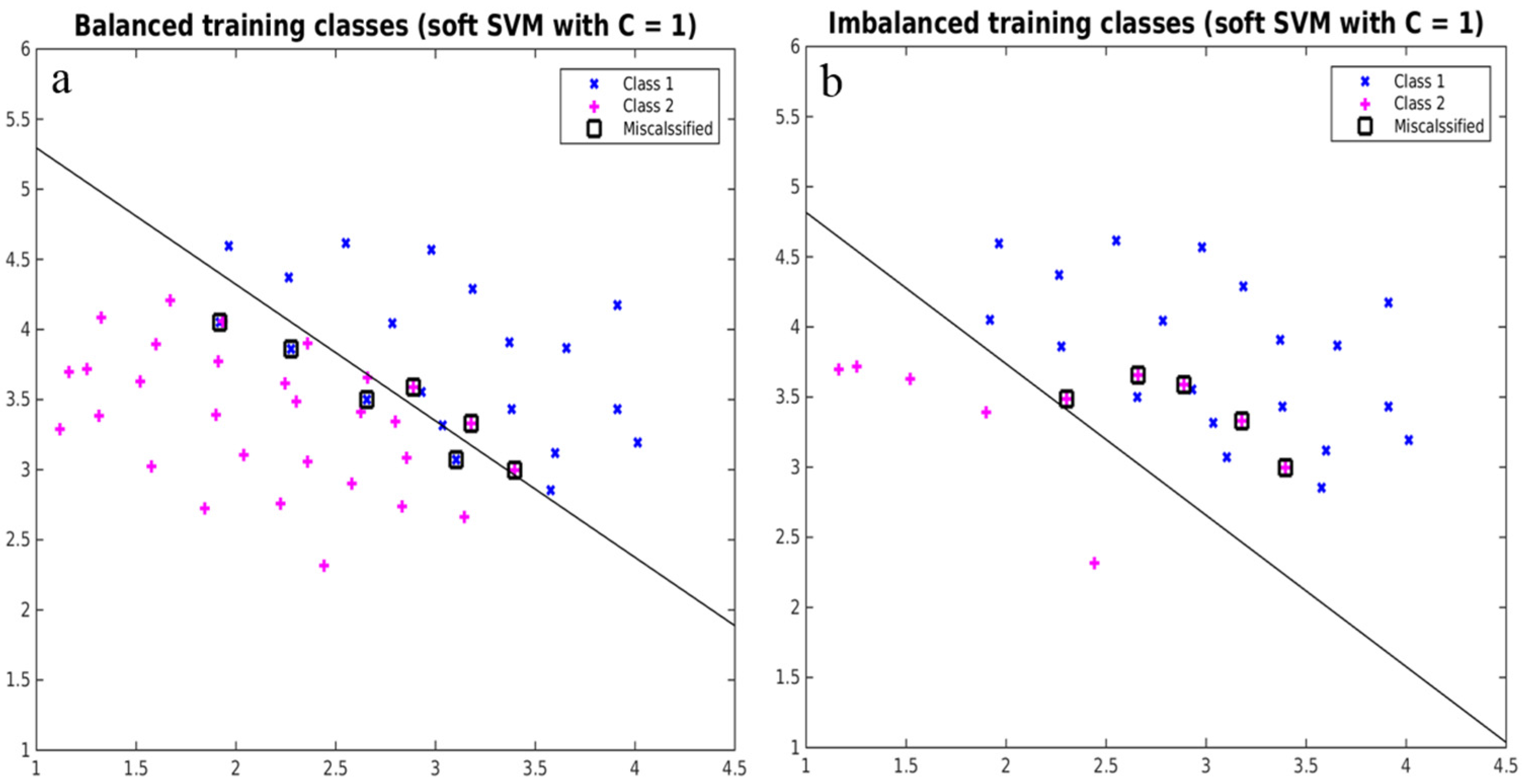
2.5. Implementing Strategies to Overcome Imbalance

We implemented simple strategies for alleviating difficulties posed by imbalanced training data that represent two primary ways for overcoming imbalance; a data based approach to manipulate the input data, and a cost based approach to modify the classification decisions when the model is presented with imbalanced data [21]. The first strategy created a dataset with equal sample sizes for all classes by randomly subsampling all classes to equal the sample size of the smallest class (downsampling). The major drawback of this method is the removal of potentially valuable data points, but there is considerable research in improved methods of data selection, including use in application to hyperspectral species classification (see Section 4.2). The second strategy maintained the full set of data and accounted for differences in sample sizes by allowing a different cost parameter for each pair of the classes [49]. In this way, the common classes maintained their large sample size, but the decision boundary between a majority and minority class pairs was shifted towards the majority class.

We ran four variations of a 20-species SVM classification model that differed in the input data or the algorithm itself (Table S1). For these tests, the mixed-species “Others” class was not included. The first variation, referred to as “Full” model, included all field data for 20 species. The sample size for each species varied from 20–116, with 890 total crowns. The next three model variations were run on a subset of the full data, where crowns were randomly drawn from the full dataset. Each model iteration was trained and tested in the same manner as the ‘Full’ model, but was repeated 10 times to allow for a different random sample of the data to be tested.

The second variation, referred to as “Even”, had a standardized sample size, where we randomly selected 20 crowns for each species, for a total of 400 crowns. This variation represents the strategy of overcoming class imbalance by randomly undersampling (downsampling) the majority classes. The third variation referred to as “Imbalanced” had the same total number of crowns as the even sample (400), but we replicated the class imbalance of the full data, for a species sample size from 9–52 crowns. This was done to directly compare the results of an imbalanced versus balanced training dataset without the results confounded by a difference in the total sample size in the model. The fourth variation, referred to as “Weighted”, had the same input data as the “Imbalanced” variation, but weights were added to the classification algorithm. Each species was given a weight that was inversely proportional to its crown abundance in the training data. The weights were implemented when running the SVM algorithm after the training data has been split into the training and testing groups. Therefore, the class weights were generated based on the training data for each model iteration rather than based on the abundance of all crowns in the field data.

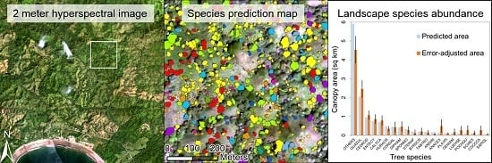
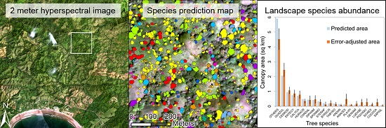
2.6. Species Predictions across the Landscape

A watershed segmentation algorithm was performed on the canopy surface model to separate tree crowns based on the height profile of the canopy [50]. Because the focus of this study was on agricultural trees rather than trees found in closed canopy forests, we identified agricultural trees based on the percent of shared edges between each segmented tree crown polygon. All polygons with greater than 65% shared edge, which indicated these crowns were surrounded closely by other tree crowns, were removed from the analysis. The segmentation performed well in areas with isolated trees because of the high contrast between the tree canopy and the surrounding grassy vegetation (Figure S4).

A final un-weighted SVM model was trained on the dataset that included all crowns (n = 1112) from the 20 individual species and 1 mixed-species class. Before the SVM classification algorithm was applied to the segmented crowns, the pixels were passed through the same NDVI and NIR filters as the training data. The NIR and NDVI filter largely removed tree crowns that were obscured by clouds or their shadows, crowns that were shaded by other crowns or located in a topographic shadow, or crowns with low leaf material. As in the training of the model, a majority vote was used to determine the crown level species prediction. Species abundance was calculated by summing the area of all crowns for each species.

The predicted area for each class was adjusted to incorporate misclassification of the model using the method presented by Olofsson et al. [51]. This approach generates an error matrix of estimated area proportions using an error matrix from an accuracy assessment of the model and the predicted area of each class. While the error matrix used to generate error-adjusted class area ideally would be developed from an independent stratified random sampling of the predicted species map [52], this was unavailable due to difficulty in accessing many areas of this large landscape in the field (see Section 4.4). Instead, we used a crown-level error matrix from one of the 30 iterations of the model. The model iteration used had the median overall accuracy. The error-adjusted class areas were calculated as:

$${\widehat{A}}_j=A_{tot}{\displaystyle \sum }_i{W}_i\frac{n_{ij}}{n_{i·}}$$

(3)

where ${\widehat{A}}_j$ is the unbiased estimator of class j, $A_{tot}$ is the total predicted area of all classes, $W_i$ is the proportional area of class j in the predicted map, $n_{ij}$ is the proportional area of predicted class i that is truly class j, and $n_{i·}$ is the proporational area of class i in the prediction map. Standard error of the adjusted area was also calculated for each class (see full calculations in [51]).

3. Results

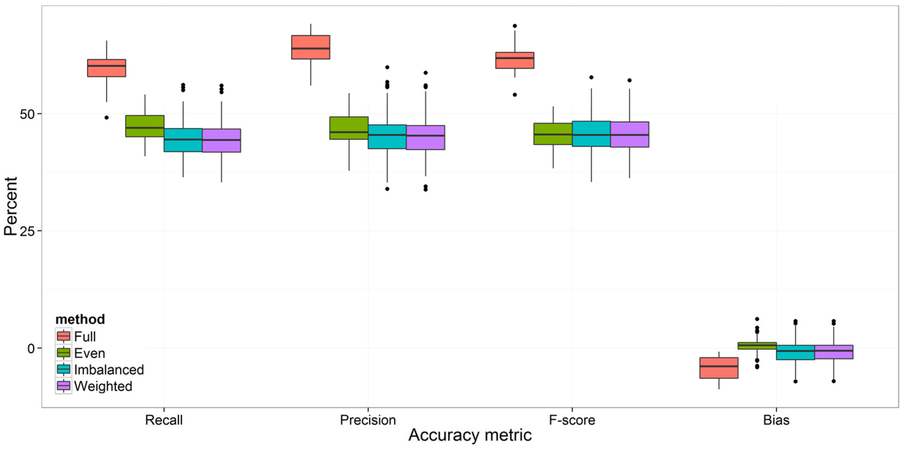
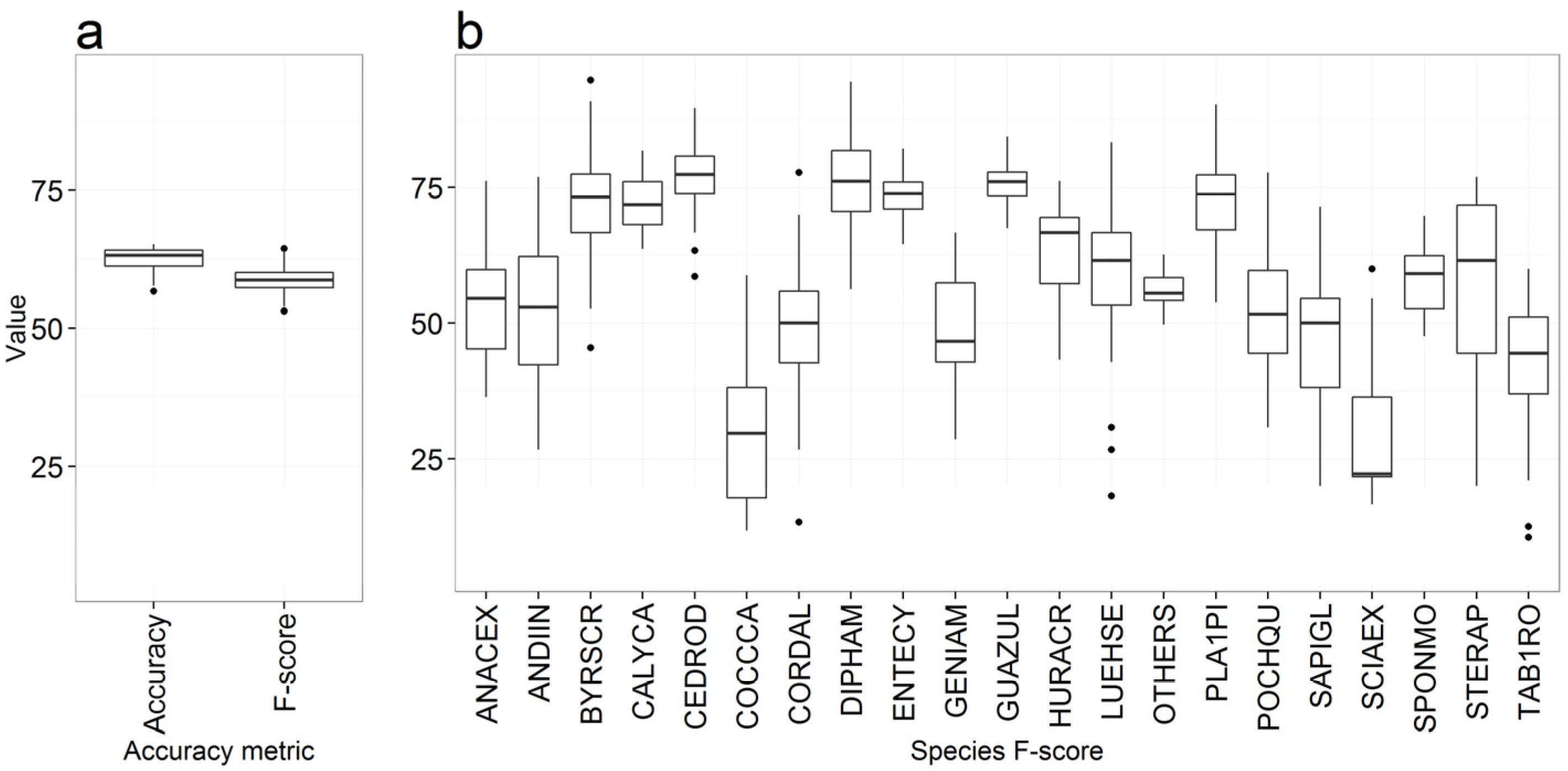
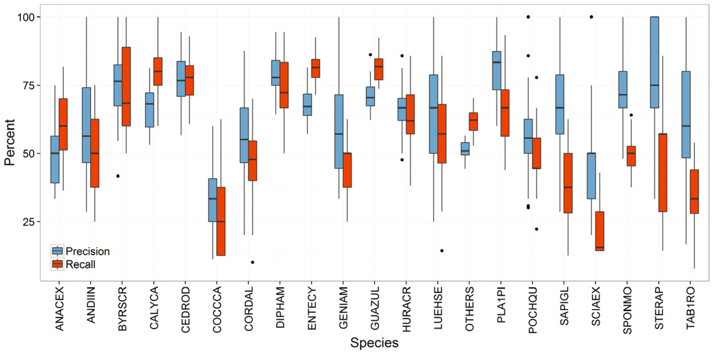
3.1. Overall Accuracy and F-score

The SVM model run on the full set of data with 21 species-classes had a mean overall accuracy across 30 iterations of 62% ± 2.3% (Figure 3a). The mean species F-score, which takes into account differences between precision and recall accuracy, was 59% ± 2.7%. Species-level measures of the F-score ranged from 10%–95%, with high variability seen within and across species (Figure 3b). Species with high accuracy and low variability across iterations were Cedrela odorata, Enterolobium cyclocarpum, and Guazuma ulmifolia which were the three most abundant species in the training data set. The multiclass “Others” also had low variability across iterations, but accuracy was considerably lower than many other species at 57%.

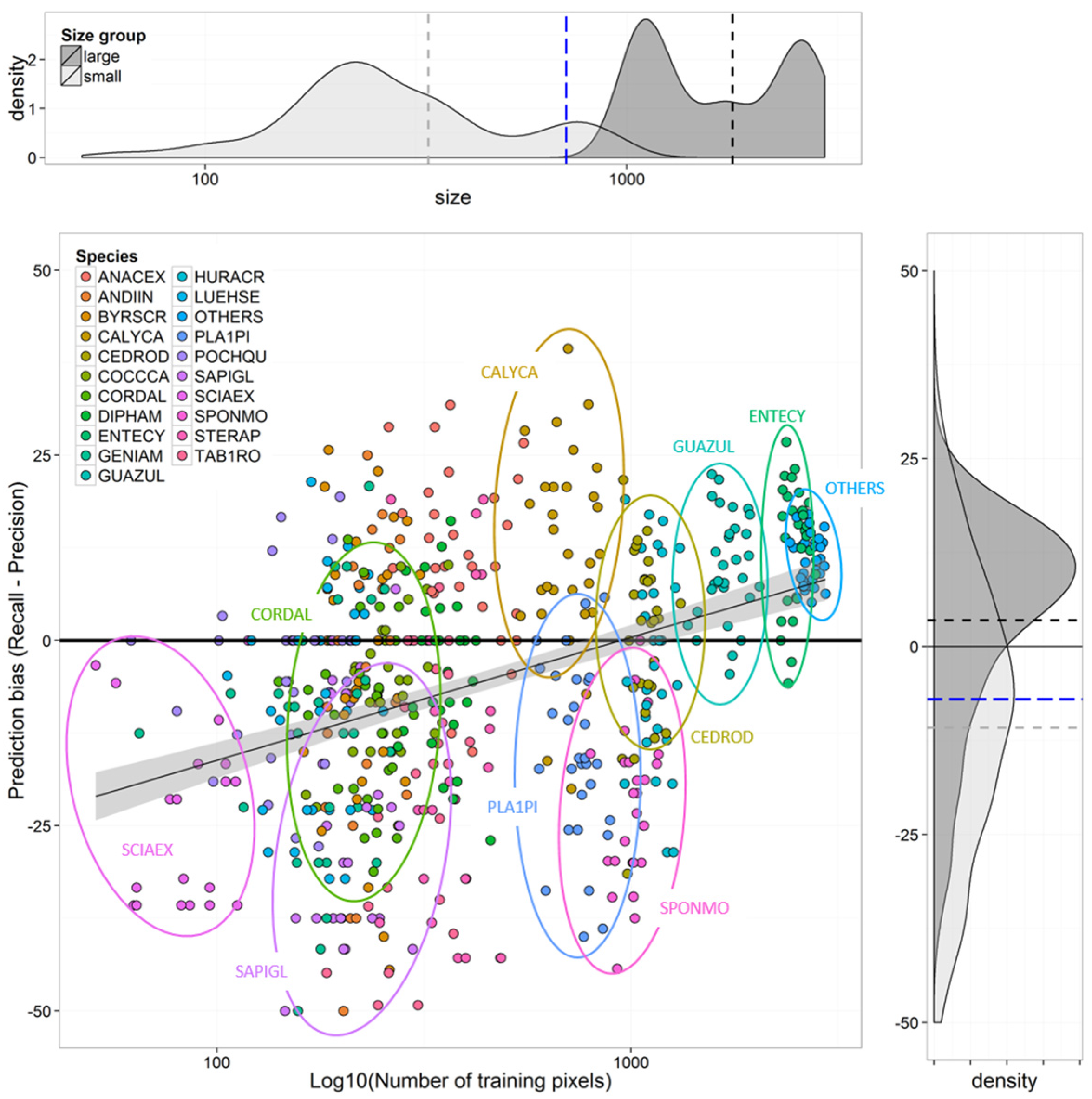
Species Prediction Errors

The differences between precision and recall for each species were highly variable, both in the level of accuracy for each metric and in which metric was greater (Figure 4). Species with higher values of both precision and recall (Calycophyllum candidissimum, E. cyclocarpum., G. ulmifolia and the mixed-species class) tended to have higher recall relative to precision, but there were exceptions to this trend (ex. Diphysa americana). Species with high recall relative to precision were shown to have many commission errors, where predictions of those species belonged to other classes (see confusion matrix in Figure S5). Most species had high precision relative to recall, driven by the commission errors of the “Others” class. Only one species (C. odorata) had a both high precision and recall, which was reflected in its high F-score (Figure 3).

The difference in prediction error (prediction bias), calculated as commission minus omission errors (or recall minus precision), ranged from −87% to +40%. Across all species, the mean prediction bias was −7%. When grouping the species into small or large classes based on a 1000 pixel threshold, the large classes had a mean prediction bias of 4% whereas the small classes had a mean prediction bias of −11% (Figure 5).

Prediction bias and had a significant positive relationship with the sample size of the training data (Figure 5). Across 1000 random tests of the linear model, the mean R² was 13% ± 3%, meaning that 13% the variation in the prediction bias was explained by sample size alone. While most species spanned a large range of prediction bias across iterations, a few species were consistently positive or negative. Enterlobium cyclocarpum, G. ulmifolia, and the “Others” had the large class sizes and positive prediction bias, which indicated these classes are generally over predicted in the classification model. While species with smaller class sizes showed high variability in prediction bias, some of these species, such as Cordia allidora, Sapium glandulosum, and Sciadodendron excelsum, tended to have negative prediction bias. This trend indicates that species with smaller sample sizes are underpredicted in classification models. There were a few notable exceptions to this trend, particularly C. candidissimum which had high recall and relatively low precision, resulting in strong positive prediction bias, and Platymiscium pinnatum and Spondias mombin, which had strong negative prediction bias.

The linear trend in prediction bias with training data size was not unique to our study. In a classification of 15 species plus one mixed-species class of African savanna species [29], despite having a low level of class imbalance relative to this study (Figure S1), the prediction bias showed a positive relationship with the relative class sample size (Figure S6). While the largest mixed-species class was the only class with high positive bias, the other single-species classes showed the positive trend despite all being under predicted.

3.2. Strategies for Model Improvement

Downsampling, which reduced the sample size of the species with large classes so all class sizes were equal (Even variation) decreased model-level precision, recall, and F-score by 12%, 17%, and 16% respectively, compared to the full dataset (Full variation, Figure 6). Down-sampling also increased the prediction bias from −4% in the Full variation to near 0% in the Even variation. The differences between the model results for the Full and Even variations reflected differences in both the total number of crowns in the model and the degree of class imbalance (Table S1).

Model recall and precision were significantly higher for the Even variation than the Imbalanced variation, but no difference was seen in model F-score. The Imbalanced data also had a significantly more negative prediction bias than the Even model, at −0.86% and 0.42%, respectively. Because the total number of crowns between the Even and the Imbalanced variations was the same (400 crowns), differences between these model variations reflected differences in the relative sample sizes for each class.

While the differences in recall, precision, F-score, and bias between the Imbalanced and Weighted variation were significant when compared with a paired t-test, the percent difference was very small. Therefore, adjusting the model prediction to account for differences in class sizes did not result in a model with higher accuracy and lower bias.

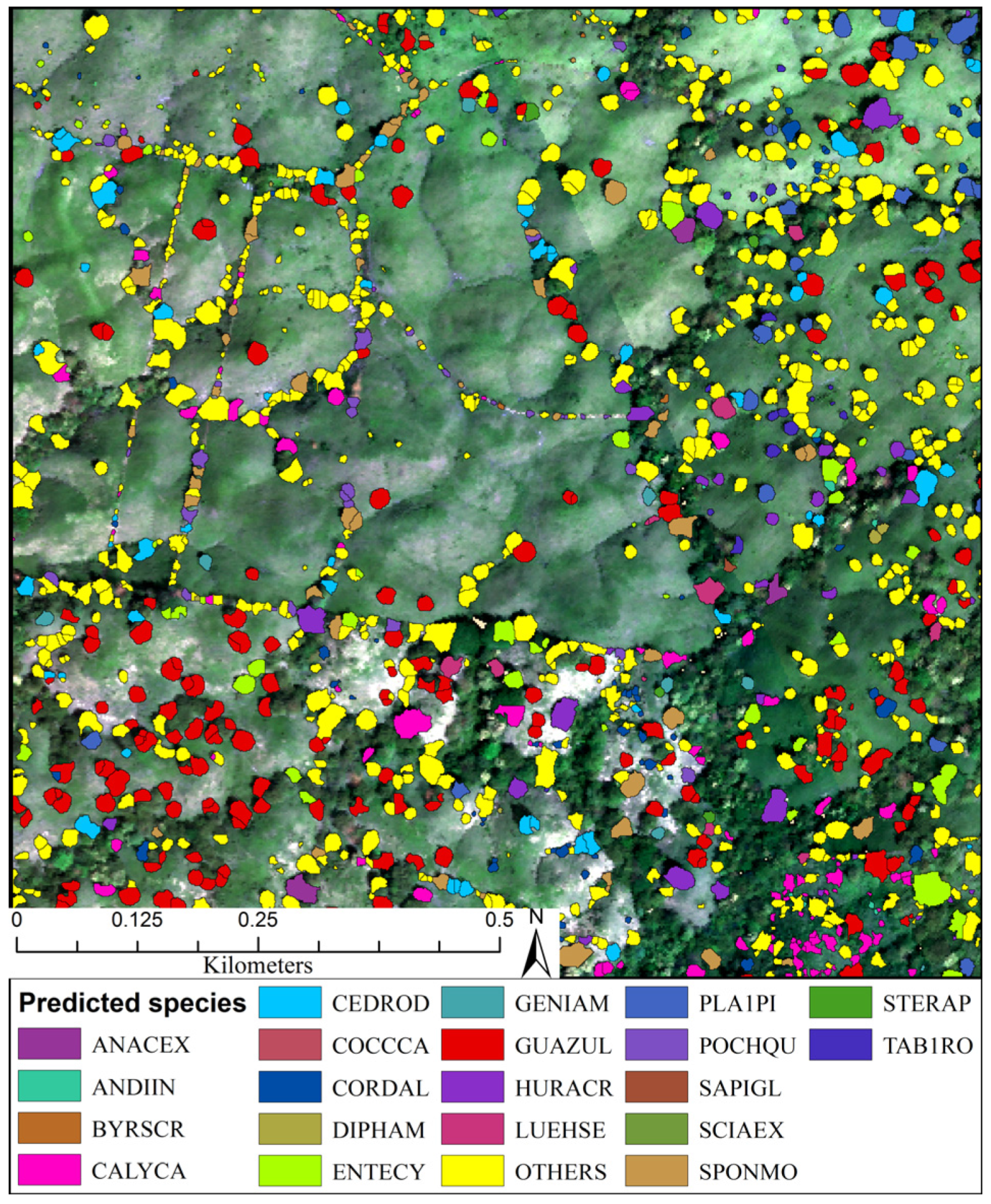
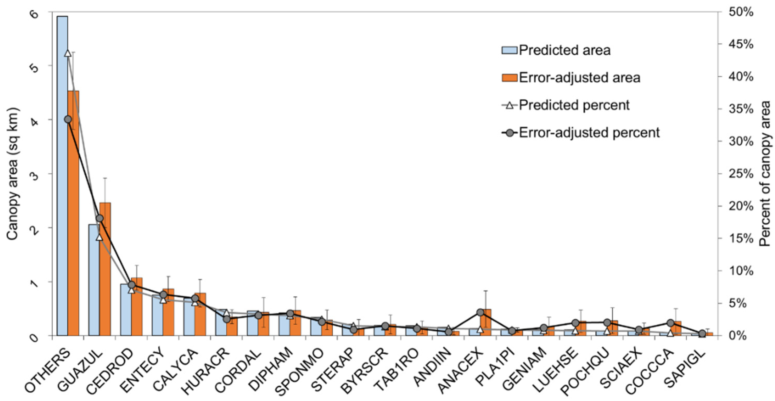
3.3. Predicted Landscape Species Distributions

Application of the classification model to 200,000 automatically delineated crown polygons of agricultural trees produced a predicted species map of individual trees across a 23,000 ha landscape (Figure 7). The predictions of species for individual crown polygons highlights the species composition and diversity of different types of agricultural tree cover (live fences or isolated pasture trees), and spatial patterns of different species, such as clumping of Guazuma ulmifolia.

Across the 23,000 ha landscape, the mixed-species “Others” class was the most abundant species on the landscape at 44% of the predicted area (Figure 8). The five most abundant species on the landscape (excluding the “Others” class) represented 37% of the landscape area. Pachira quinata was only predicted at 0.7% of the landscape, but because there were many deciduous P. quinata individuals at the time when the images were taken, it is likely that many individual of this species were removed from the prediction because the crowns had low NDVI and NIR reflectance.

Correcting the abundance predictions with the prediction errors reduced the abundance of the the most common class and increased the abundance of the other classes. In the corrected abundance predictions, the “Others” class was reduced from 6 sq km to 4.5 ± 0.7 sq·km., which is a reduction in percent canopy cover by 11%, from 44% to 33%. The abundance of the next five most abundant species increased from 36% to 41% of the landscape. As a result, the more rare species (15 least abundant species) increased from a predicted abundance of 20% to 26% (3.5 sq·km).

4. Discussion

4.1. Effects of Imbalanced Data on Model Performance and Species Predictions

We have applied evaluation tools to quantify the effect of widely differing training class sizes for species classification from imaging spectroscopy data (hyperspectral imagery) and generated landscape species abundance distributions, which have been adjusted to account for model error. The overall accuracy of the 21-class model was 62% ± 2.3% and the F-score was 59% ± 2.7%. This level of accuracy is consistent with other studies using similar classification algorithms and numbers of tropical tree species [16]. While our study quantified the accuracy achieved with the classification of a large number of species, we also estimated the abundance of species on the landscape by incorporating model omission and commission errors into analysis of landscape species distributions.

Our classification model with imbalanced data suggests that while more common species were overrepresented in the model predictions for the test dataset, this had a small effect on the landscape species distributions. First, species that were more common on the landscape had greater representation in the field dataset used to develop the model because of the frequency at which they are encountered. Our field data required four months of fieldwork and included 1140 individuals from 76 species resulting in a labeled dataset that was highly imbalanced despite attempts to increase samples of rare species and map fewer common species. The range in class sample size was 20–222 crowns; a level imbalance which is evident in other studies as well (Table 1, Figure S1). Second, our results showed that species with larger sample sizes tend to have positive prediction bias (commission errors were greater than omission errors) and species with small sample sizes had negative prediction bias (Figure 5). This generalization is supported in the confusion matrix (Figure S5) with many individuals of rarer species being incorrectly predicted as a few common classes (mixed-species class, C. odorata, E. cyclocarpum, G. ulmifolia). This trend is not unique to our study. Despite having a relatively low class imbalance as compared with this and other studies, the results from Colgan et al. [29] show that prediction bias had a significantly positive relationship with the number of crowns in the training data with an over prediction of 34% for the class with the largest sample size (Figure S6).

The positive relationship in this study between sample size and prediction bias is likely due to both how the optimal value of the SVM’s cost parameter was chosen, and the fact that the cost parameter is fixed across all one-against-one species comparisons. The optimal values for the cost and the width parameters were chosen that minimized the overall model error, or the number of misclassifications across all class comparisons. This is the optimization method for tuning the SVM parameters used in most applications. Because the optimization criterion was the total number of misclassifications across all species, the species with larger class size held greater weight in defining this error than species with smaller class sizes. An alternative strategy for parameter optimization is to reduce the effect of class imbalance is to select the parameters that minimized average model error where each species is weighted equally, or to use a different metric such as Balanced Accuracy or the F-score [11,13].

Despite the trends we found in prediction bias, incorporating model errors with the predicted class areas do not remarkably change the landscape predictions of species abundance (Figure 8). While individual predictions of tree species identity could not be corrected in the map, the overall landscape abundances were adjusted by knowing the over and underestimation. Accounting for prediction errors in the landscape species distribution primarily resulted adjustements for the first and second most common classes and minimal changes for all other classes.

4.2. Selection of Training Data for Optimal Species-Level Accuracy

When standardizing the training data size across classes, we found that the degree of bias in the model was reduced, but the overall accuracy was significantly reduced from the model that used the full dataset (Figure 6). One potential way to avoid the reduction in overall accuracy, is to adapt available methods to reduce the size of large species classes while maintaining the full range of spectral variaiblity in that class. This has been done for species classification using spectral mixture analysis and discriminant analysis [26,53]. For SVM algorithms, spectral variability can be maintined while reducing large data classes with numerous methods to balance the data [49], by choosing only data points on the border between classes to define the separation between classes [22], or iteratively pruning the support vectors to achieve the best separation between classes [54]. Other approaches to manipulate the SVM algorithm by adjusting margin calculation or variable mis-classification costs is also an active area of research [44]. The implications for these selection processes on bias in the final model and subsequent application to large areas with multiple classes has not been quantified.

4.3. Minimum Sample Size Threshold

A important question in the development of operational species mapping in the tropics is what amount and type of data are necessary to achieve sufficient classification accuracy [15]. This question is especially relevant in diverse landscapes where locating and hand-mapping individuals of rare species may be difficult. A better understanding of the effect of class sample sizes on accuracy can help focus field data collection campaigns. We found that species with small sample sizes, as a result of these species being uncommon on the landscape, had high variability in accuracy/error across all iterations (Table 2, Figure 3 and Figure 4). These species include Coccoloba caracasana, Genipa americana, and S. excelsum. Prediction bias was also highly variable across all 30 iterations for species with fewer than 1200 pixels (Figure 5). Species that are relatively uncommon but have high accuracy, such as P. quinata and Byrsonima crassifolia with high value and multiple uses [19,20], can be useful for large scale monitoring and conservation efforts. Whereas Baldeck and Asner [15] suggest approximately 20 crowns as the focal number to achieve optimal classification accuracy in an 11-class model, our results suggest that in a model with 21 classes, all classes should have at least 20–30 individual crowns per class to produce accurate and reliable classification predictions, allowing for a split of the crowns into training and test groups. However, as has been discussed in other studies, the amount of training data to achieve maximum accuracy is dependent on the number of species to be classified and their spectral separability given the spectral and spatial resolution of the data [15].

4.4. Operational Species Mapping in Species-Rich Landscapes

Our study contributes to operational biodiversity mapping in species-rich landscapes because we have done our analysis at the scale of individual crowns, we have included most species in our model that exist on the landscape, and we highlight a way in which classification accuracy can be communicated and used in secondary analysis of species predictions. Examples of ecological applications that could utilize the type of operational species mapping presented in this study are those that assess patterns of species composition and abundance across environmental gradients or land management units, identification of areas of high or low tree cover and species diversity, developing or parameterizing forest succession models, and providing landscape estimates of aboveground biomass. For more focused applications where accurate predictions of species location and identiy is needed, such as monitoring rare or ecologically important species (Ex. Tabebuia rosea), classification and mapping errors may be too large. For these applications, techniques such as semi-supervised methods where a focal group of species is identified from a background of unknown species [11,13,55], may be a better approach.

In this study (also see [29]) all species with very small sample sizes were pooled into a single mixed-species class (“Other”), which consequently became the class with the largest sample size and the greatest predicted abundance on the landscape. Creating an “Other” class allowed for the inclusion of 44 species in the model that had small sample sizes. This method was done to allow for less frequently encountered species to be included in the model. In this way, many relatively rare species could be mapped, albeit individual species distinctions could not be made. Despite the advantage of doing this to allow for species predictions of less common species, creating this group that contained many species may not be desirable for several reasons. Because this class is composed of many species, the spectral variation within this class is likely much larger than the single-species classes. Therefore, the spectral range this class occupies is very large and may overlap other single-species classes, causing misclassification in both directions between the mixed-species class and some unique species classes (Figure S5). Also, unless every species on the landscape has been included in the training data, which is difficult in a species-rich tropical landscape, the “Other” class does not include unsampled species. A classifier such as SVM is bound to assign the unknown spectra to one of the known training classes. In this way, if pixels in the image belong to a species that was not included in the training data, those pixels are still assigned to one of the known species.

A promising way to deal with high species diversity and many rare, and potentially unsampled species, is probabilistic classifiers such probabilistic SVM [56], relevance vector machine [57], and Gaussian Process [58], which depart from the hard implementation of a supervised classification that forces all unknown data into known classes. The classifiers make soft predictions that allow a prediction to have a probability of being one species versus another, including the probability that a pixel or crown is not any of the species contained in the training data set. Therefore, species present on the landscape that were not used to train the model will not be forced into one of the known classes. Building such a soft classifier is challenging in the context of hyperspectral vegetation classification due to the high dimensionality of data and similarity of vegetation spectra.

We incorporate the model error into the predictions to gague if data imbalance affects predicted species maps. To calculate the error-adjusted areas for each class, we used the accuracy assessment data from one iteration of our model. This approach is common in species classification studies when assessing the accuracy of a classification model [3,24,26] because of the difficulty in visiting individual trees across the landscape, especially after the prediction map has been generated.

It was not possible in this study to implement a randomization scheme for collecting field data. This is often the case in tropical forests because of difficulty of access because of lack of insfrastructure and difficult terrain. Furthermore, species classifications differ from land-use/land-cover determination, because the species identity of an individual tree cannot be determined from remote images, such as aerial photos or high resolution remote sensing. To determine species in a tropical environment, the tree must be visited and identified by a trained botanist. The logistic and financial constraints limit the development of an ideal assessment dataset [52]. The difficulty in accessing all regions of the tropical landscape highlights the need for remote detection of species.

Despite not having a randomized validation set of the prediction map, we use one of many methods [59] to incorporate estimates of map error from the accuracy assessment of our classification model to provide an estimate of the abundance of species on the landscape. These data are stratified relative to their abundance in the field data, which is consistent with the relative abundances of species on the landscape. While the error-adjusted area did change the shape and evenness of the species rank curve relative to the predicted area (Figure 8), these shifts were primarily driven by differences for the two most common species.

4.5. Operational Species Mapping Provides a View of the Diverse Tropical Landscape

Despite the drawbacks mentioned above of the methodology used in this study, the species classification developed here could be used to gain insight into the tree species composition of a 23,000 ha agricultural landscape of the southern Azuero peninsula that cannot be easily obtained from field sampling. We compared the results of this study to those of Griscom et al. [20] who directly inventoried tree species in 8 ha of active and abandoned pastures. The 8 ha were sampled from an 85 ha cattle farm and an adjacent 100 ha of secondary forests and abandoned pasture, which is a large plot size for field sampling of forest inventory.

Our study estimates that the most common species on the landscape were G. ulmifolia (18% of the species abundance measured by crown area after error correction), C. odorata (8%), E. cyclocarpum (6%), and C. candidissimum (6%). In the 185-ha property in the Azuero Peninsula [20], G. ulmifolia and C. allidora were much more dominant than our estimate, representing 63% of the individuals in the active pastures. Furthermore, G. ulmifolia was the dominant species in the 2-year and 5-year abandoned pastures at 92% and 37% of the species, respectively. Our prediction map suggests that G. ulmifolia, whose seeds are eaten and dispersed by cattle, may be spatially clumped (Figure 7). Consequently, while there may be high density of G. ulmifolia individuals in a pasture that is actively grazed, or recently abandoned, they are found at lower numbers across the entire landscape. Enterolobium cyclocarpum was also predicted to be a dominant part of the landscape in our analysis, but was absent in the field inventory. This species is well known for growing in open landscapes and producing a broad crown which provides shade for cattle.

Both this study and Griscom et al. [20] point to the high diversity of the Azuero landscape, which is highly deforested and dominated by pasture. Griscom et al. [20] highlight the range in species diversity across different habitat types, and found 25 species in active pastures, 3 species in two-year abandoned pastures, and 12 species in five-year abandoned pastures. In our landscape prediction of the abundances of 20 of the most common species (plus a mixed group representing an additional 24 species) on the landscape, a species that did not occur in the large 185-ha area sampled (E. cyclocarpum) was one of the most dominant across the 23,000 ha landscape. Our landscape species prediction also showed that the distributions of the most dominant species, although widespread, are clumped and thus are not well-characterized by a simple large field plot. We extend the conclusion by Griscom et al. [20] in recognizing the variation in species abundance across the landscape. The spatial prediction map produced by classification of imaging spectroscopy data can allow for direct inventory of species and identifying land parcels that have a scarcity of trees or low diversity as areas where active restoration needs to occur. Work to incorporate species predictions in forest succession modeling and conservation planning can utilize species prediction maps.

5. Conclusions

Generating landscape scale maps of individual tree species allows for a variety of applications relevant to ecology and conservation such as the evaluation of spatial patterns in tropical tree distributions [3], focusing conservation efforts in areas with relatively high tree diversity or rare species, and informing forest succession models to predict the forest composition of the future landscape [37]. However, these ecologically relevant applications rest on species classification models that are not perfect, but have known prediction errors. Our study quantified species-level accuracy and errors associated with training an SVM model with imbalanced data. While this study shows that 21 species-classes can be predicted with an accuracy of 62%, it highlights the need to consider species-level differences in prediction errors that may affect predicted species patterns across the landscape, the degree to which depends on the ultimate application or question of interest. Species classifications will become more widely implemented as the availability of hyperspectral image data increases. While methods continue to be developed to overcome some of the current challenges caused by imbalanced data, we stress the need to report errors of different types (omission and commission) in species classification models, and to incorporate these errors into secondary analysis of landscape species distribution and abundance patterns. This study provides species abundance estimates from the application of a species classifier to a large area (23,000 ha) that are distinctly different from those of a field study of a 185-ha area, and reveal a diverse tropical agricultural landscape. Further analyses of species distributions across the landscape can contribute to our understanding of human or environmental effects on species composition, in addition to focusing conservation efforts in areas with high tree cover and diversity.

References

1. Nagendra, H. Using remote sensing to assess biodiversity. Int. J. Remote Sens. 2001, 22, 2377–2400. [Google Scholar] [CrossRef]
2. Turner, W.; Spector, S.; Gardiner, N.; Fladeland, M.; Sterling, E.; Steininger, M. Remote sensing for biodiversity science and conservation. Trends Ecol. Evol. 2003, 18, 306–314. [Google Scholar] [CrossRef]
3. Colgan, M.S.; Asner, G.P. Coexistence and environmental filtering of species-specific biomass in an African savanna. Ecology 2014, 95, 1579–1590. [Google Scholar] [CrossRef] [PubMed]
4. Condit, R. Spatial patterns in the distribution of tropical tree species. Science 2000, 288, 1414–1418. [Google Scholar] [CrossRef] [PubMed]
5. Lucas, R.; Bunting, P.; Paterson, M.; Chisholm, L. Classification of Australian forest communities using aerial photography, CASI and HyMap data. Remote Sens. Environ. 2008, 112, 2088–2103. [Google Scholar] [CrossRef]
6. Ustin, S.L.; DiPietro, D.; Olmstead, K.; Underwood, E.; Scheer, G.J. Hyperspectral remote sensing for invasive species detection and mapping. IEEE Int. Geosci. Remote Sens. Sympos. 2002, 3, 1658–1660. [Google Scholar]
7. Underwood, E.; Ustin, S.; DiPietro, D. Mapping nonnative plants using hyperspectral imagery. Remote Sens. Environ. 2003, 86, 150–161. [Google Scholar] [CrossRef]
8. He, K.S.; Rocchini, D.; Neteler, M.; Nagendra, H. Benefits of hyperspectral remote sensing for tracking plant invasions. Divers. Distrib. 2011, 17, 381–392. [Google Scholar] [CrossRef]
9. Clark, M.L.; Roberts, D.A.; Clark, D.B. Hyperspectral discrimination of tropical rain forest tree species at leaf to crown scales. Remote Sens. Environ. 2005, 96, 375–398. [Google Scholar] [CrossRef]
10. Nagendra, H.; Rocchini, D. High resolution satellite imagery for tropical biodiversity studies: The devil is in the detail. Biodivers. Conserv. 2008, 17, 3431–3442. [Google Scholar] [CrossRef]
11. Baldeck, C.A.; Asner, G.P.; Martin, R.E.; Anderson, C.B.; Knapp, D.E.; Kellner, J.R.; Wright, S.J. Operational tree species mapping in a diverse tropical forest with airborne imaging spectroscopy. PLoS ONE 2015, 10, e0118403. [Google Scholar] [CrossRef] [PubMed]
12. Alonzo, M.; Bookhagen, B.; Roberts, D.A. Urban tree species mapping using hyperspectral and lidar data fusion. Remote Sens. Environ. 2014, 148, 70–83. [Google Scholar] [CrossRef]
13. Féret, J.B.; Asner, G.P. Semi-supervised methods to identify individual crowns of lowland tropical canopy species using imaging spectroscopy and lidar. Remote Sens. 2012, 4, 2457–2476. [Google Scholar] [CrossRef]
14. Cochrane, M.A. Using vegetation reflectance variability for species level classification of hyperspectral data. Int. J. Remote Sens. 2000, 21, 2075–2087. [Google Scholar] [CrossRef]
15. Baldeck, C.A.; Asner, G.P. Improving remote species identification through efficient training data collection. Remote Sens. 2014, 6, 2682–2698. [Google Scholar] [CrossRef]
16. Féret, J.B.; Asner, G.P. Tree species discrimination in tropical forests using airborne imaging spectroscopy. IEEE Trans. Geosci. Remote Sens. 2012, 51, 1–12. [Google Scholar] [CrossRef]
17. Alonzo, M.; Roth, K.; Roberts, D. Identifying Santa Barbara’s urban tree species from AVIRIS imagery using canonical discriminant analysis. Remote Sens. Lett. 2013, 4, 513–521. [Google Scholar] [CrossRef]
18. Pitman, N.C.A.; Terborgh, J.W.; Silman, M.R.; Núñez, P.V.; Neill, D.A.; Cerón, C.E.; Palacios, W.A.; Aulestia, M. Dominance and distribution of tree species in upper Amazonian terra firme forests. Ecology 2001, 82, 2101–2117. [Google Scholar] [CrossRef]
19. Love, B.; Spaner, D. A survey of small-scale farmers using trees in pastures in Herrera Province, Panama. J. Sustain. For. 2005, 20, 37–65. [Google Scholar] [CrossRef]
20. Griscom, H.P.; Connelly, A.B.; Ashton, M.S.; Wishnie, M.H.; Deago, J. The structure and composition of a tropical dry forest landscape after land clearance; Azuero peninsula, Panama. J. Sustain. For. 2011, 30, 37–41. [Google Scholar] [CrossRef]
21. Sun, Y.; Wong, A.K.; Kamel, M.S. Classification of imbalanced data: A review. Int. J. Pattern Recognit. Artif. Intell. 2009, 23, 687–719. [Google Scholar] [CrossRef]
22. Foody, G.M.; Mathur, A. Toward intelligent training of supervised image classifications: Directing training data acquisition for SVM classification. Remote Sens. Environ. 2004, 93, 107–117. [Google Scholar] [CrossRef]
23. Dalponte, M.; Bruzzone, L.; Gianelle, D. Tree species classification in the Southern Alps based on the fusion of very high geometrical resolution multispectral/hyperspectral images and lidar data. Remote Sens. Environ. 2012, 123, 258–270. [Google Scholar] [CrossRef]
24. Cho, M.A.; Mathieu, R.; Asner, G.P.; Naidoo, L.; van Aardt, J.; Ramoelo, A.; Debba, P.; Wessels, K.; Main, R.; Smit, I.P.J.; et al. Mapping tree species composition in South African savannas using an integrated airborne spectral and lidar system. Remote Sens. Environ. 2012, 125, 214–226. [Google Scholar] [CrossRef]
25. Knudby, A.; Nordlund, L.M.; Palmqvist, G.; Wikström, K.; Koliji, A.; Lindborg, R.; Gullström, M. Using multiple Landsat scenes in an ensemble classifier reduces classification error in a stable nearshore environment. Int. J. Appl. Earth Obs. Geoinf. 2014, 28, 90–101. [Google Scholar] [CrossRef]
26. Roth, K.L.; Dennison, P.E.; Roberts, D.A. Comparing endmember selection techniques for accurate mapping of plant species and land cover using imaging spectrometer data. Remote Sens. Environ. 2012, 127, 139–152. [Google Scholar] [CrossRef]
27. Jones, T.G.; Coops, N.C.; Sharma, T. Assessing the utility of airborne hyperspectral and lidar data for species distribution mapping in the coastal Pacific Northwest, Canada. Remote Sens. Environ. 2010, 114, 2841–2852. [Google Scholar] [CrossRef]
28. Clark, M.L.; Roberts, D.A. Species-Level Differences in Hyperspectral Metrics among Tropical Rainforest Trees as Determined by a Tree-Based Classifier. Remote Sens. 2012, 4, 1820–1855. [Google Scholar] [CrossRef]
29. Colgan, M.S.; Baldeck, C.A.; Féret, J.-B.; Asner, G.P. Mapping savanna tree species at ecosystem scales using support vector machine classification and BRDF correction on airborne hyperspectral and lidar data. Remote Sens. 2012, 4, 3462–3480. [Google Scholar] [CrossRef]
30. Melgani, F.; Bruzzone, L. Classification of hyperspectral remote sensing images with support vector machines. IEEE Trans. Geosci. Remote Sens. 2004, 42, 1778–1790. [Google Scholar] [CrossRef]
31. Pal, M.; Mather, P.M. Support vector machines for classification in remote sensing. Int. J. Remote Sens. 2005, 26, 1007–1011. [Google Scholar] [CrossRef]
32. Shao, Y.; Lunetta, R.S. Comparison of support vector machine, neural network, and CART algorithms for the land-cover classification using limited training data points. ISPRS J. Photogramm. Remote Sens. 2012, 70, 78–87. [Google Scholar] [CrossRef]
33. He, H.; Garcia, E.A. Learning from Imbalanced Data. IEEE Trans. Knowl. Data Eng. 2009, 21, 1263–1284. [Google Scholar]
34. Blagus, R.; Lusa, L. Class prediction for high-dimensional class-imbalanced data. BMC Bioinform. 2010, 11, 523. [Google Scholar] [CrossRef] [PubMed]
35. Lin, W.J.; Chen, J.J. Class-imbalanced classifiers for high-dimensional data. Brief. Bioinform. 2013, 14, 13–26. [Google Scholar] [CrossRef] [PubMed]
36. Shao, G.; Wu, J. On the accuracy of landscape pattern analysis using remote sensing data. Landsc. Ecol. 2008, 23, 505–511. [Google Scholar] [CrossRef]
37. Peterson, C.J.; Dosch, J.J.; Carson, W.P. Pasture succession in the Neotropics: Extending the nucleation hypothesis into a matrix discontinuity hypothesis. Oecologia 2014, 175, 1325–1335. [Google Scholar] [CrossRef] [PubMed]
38. Olson, D.M.; Dinerstein, E.; Wikramanayake, E.D.; Burgess, N.D.; Powell, G.V.N.; Underwood, E.C.; D’amico, J.A.; Itoua, I.; Strand, H.E.; Morrison, J.C.; et al. Terrestrial Ecoregions of the World: A New Map of Life on Earth. Bioscience 2001, 51, 933–938. [Google Scholar] [CrossRef]
39. Asner, G.P.; Knapp, D.E.; Boardman, J.; Green, R.O.; Kennedy-Bowdoin, T.; Eastwood, M.; Martin, R.E.; Anderson, C.; Field, C.B. Carnegie Airborne Observatory-2: Increasing science data dimensionality via high-fidelity multi-sensor fusion. Remote Sens. Environ. 2012, 124, 454–465. [Google Scholar] [CrossRef]
40. Asner, G.P.; Martin, R.E.; Anderson, C.B.; Knapp, D.E. Quantifying forest canopy traits: Imaging spectroscopy versus field survey. Remote Sens. Environ. 2015, 158, 15–27. [Google Scholar] [CrossRef]
41. Misc functions of the Department of Statistics, Probability Theory Group (Formally: E1071), TU Wein 2015. Available online: https://cran.r-project.org/web/packages/e1071/index.html (accessed on 1 December 2015).
42. R Foundation for Statistical Computing: A Language and Environment for Statistical Computing. Available online: https://www.R-project.org (accessed on 1 December 2015).
43. Cortes, C.; Vapnik, V. Support-vector networks. Mach. Learn. 1995, 20, 273–297. [Google Scholar] [CrossRef]
44. Yang, C.-Y.; Yang, J.-S.; Wang, J.-J. Margin calibration in SVM class-imbalanced learning. Neurocomputing 2009, 73, 397–411. [Google Scholar] [CrossRef]
45. Kavzoglu, T.; Colkesen, I. A kernel functions analysis for support vector machines for land cover classification. Int. J. Appl. Earth Obs. Geoinf. 2009, 11, 352–359. [Google Scholar] [CrossRef]
46. Kim, J.-H. Estimating classification error rate: Repeated cross-validation, repeated hold-out and bootstrap. Comput. Stat. Data Anal. 2009, 53, 3735–3745. [Google Scholar] [CrossRef]
47. Sokolova, M.; Lapalme, G. A systematic analysis of performance measures for classification tasks. Inf. Process. Manag. 2009, 45, 427–437. [Google Scholar] [CrossRef]
48. Congalton, R.G. A review of assessing the accuracy of classifications of remotely sensed data. Remote Sens. Environ. 1991, 37, 35–46. [Google Scholar] [CrossRef]
49. Tang, Y.; Zhang, Y.Q.; Chawla, N.V.; Krasser, S. SVMs modeling for highly imbalanced classification. IEEE Trans. Syst. Man. Cybern. B. Cybern. 2009, 39, 281–288. [Google Scholar] [CrossRef] [PubMed]
50. Conrad, O. Module Watershed Segmentation. Available online: http://www.saga-gis.org/saga_module_doc/2.1.3/imagery_segmentation_0.html (accessed on 11 January 2016).
51. Olofsson, P.; Foody, G.M.; Stehman, S.V.; Woodcock, C.E. Making better use of accuracy data in land change studies: Estimating accuracy and area and quantifying uncertainty using strati field estimation. Remote Sens. Environ. 2013, 129, 122–131. [Google Scholar] [CrossRef]
52. Olofsson, P.; Foody, G.M.; Herold, M.; Stehman, S.V.; Woodcock, C.E.; Wulder, M.A. Good practices for estimating area and assessing accuracy of land change. Remote Sens. Environ. 2014, 148, 42–57. [Google Scholar] [CrossRef]
53. Roth, K.L.; Roberts, D.A.; Dennison, P.E.; Alonzo, M.; Peterson, S.H.; Beland, M. Differentiating plant species within and across diverse ecosystems with imaging spectroscopy. Remote Sens. Environ. 2015, 167, 135–151. [Google Scholar] [CrossRef]
54. Chen, X.; Gerlach, B.; Casasent, D. Pruning support vectors for imbalanced data classification. In Proceedings of International Joint Conference on Neural Networks, Montreal, QC, Canada, 31 July–4 August 2005; pp. 1883–1888.
55. Baldeck, C.A.; Asner, G.P. Single-species detection with airborne imaging spectroscopy data: A comparison of support vector techniques. IEEE J. Sel. Top. Appl. Earth Obs. Remote Sens. 2014, 8, 2501–2512. [Google Scholar] [CrossRef]
56. Platt, J. Probabilistic outputs for support vector machines and comparisons to regularized likelihood methods. Adv. Large Margin Classif. 1999, 10, 61–74. [Google Scholar]
57. Tipping, M.E. Sparse Bayesian learning and the relevance vector machine. J. Mach. Learn. Res. 2001, 1, 211–244. [Google Scholar]
58. Rasmussen, C.E. Gaussian processes in machine learning. In Advanced Lectures on Machine Learning; Springer Berlin Heidelberg: Heidelberg, Germany, 2004; pp. 63–71. [Google Scholar]
59. Stehman, S. V Estimating area from an accuracy assessment error matrix. Remote Sens. Environ. 2013, 132, 202–211. [Google Scholar] [CrossRef]
Figure 1. Images of the Azuero Peninsula study site. (a) Carnegie Airborne Observatory (CAO) true-color image of 23,000 ha; (b) Location of the study site; (c) Agricultural tree cover shown in a true-color image of the CAO image with 2-m spatial resolution; (d) Typical tree cover on agricultural land.
Remotesensing 08 00161 g001
Figure 2. Effect of imbalanced data on SVM decision plane. (a) Visualization of the SVM decision plane when two classes are of balanced size; (b) the decision plane when data size is imbalanced with a large number of misclassifications of the minority class.
Remotesensing 08 00161 g002
Figure 3. Model and species-level accuracy metrics of a 21-class SVM model (a) Model-level metrics of percent overall accuracy and F-score; (b) species-level F-score. Both plots show values across 30 model iterations. Full species names for each species code are given in Table 2.
Remotesensing 08 00161 g003
Figure 4. Species-level recall and precision percent accuracy across 30 model iterations. Full species names for each species code are given in Table 2. Precision is equivalent to user accuracy, recall is equivalent to producer accuracy. High precision relative to recall means the species has lower comission errors than omission errors (see S5 for example confusion matrix).
Remotesensing 08 00161 g004
Figure 5. Relationship between class sample size and model prediction bias. Line shows a linear model with 95% confidence interval around the mean. Histogram on the top (number of pixels) and left (prediction bias) show distributions of large and small species-classes based on a 1000 pixel threshold. Dashed blue lines show mean values of size and bias for all data, and light and dark grey dashed lines show means for small and large groups, respectively. Full species names for each species code are given in Table 2.
Remotesensing 08 00161 g005
Figure 6. Model-level accuracy comparison of 4 SVM models that differ in input data. Model accuracy was measured with a 3-fold cross validation method (30 model iterations). The Even, Imbalanced, and Weighted models were run on a 400 crown subset of the full 890 crowns. Ten random subsets were done for a total of 300 model iterations. Paired t-tests between Imbalanced and Weighted model variations showed significant differences between variations for the F-score and bias metrics.
Remotesensing 08 00161 g006
Figure 7. Predicted species of agricultural tree crowns on subset of the landscape. Crown predictions are overlaid on true-color 2-meter resolution image. Polygons are colored by their predicted species. Full species names for each species code are given in Table 2.
Remotesensing 08 00161 g007
Figure 8. Predicted and error-adjusted canopy area and relative species abundance (percent) of 200,000 individual tree crowns across the 23,000 ha landscape. Predicted area was calculated as the total crown area for each species from the 21-class SVM classification model. Error-adjusted area accounts for differences in species prediction errors as calculated in Equation (3) (see Olofsson et al. [51] for full methods). Points show the relative species abundance based on the predicted area (black circles) and the error-adjusted area (white triangles). Full species names for each species code are given in Table 2.
Remotesensing 08 00161 g008