Article

IKONOS Image-Based Extraction of the Distribution Area of Stellera chamaejasme L. in Qilian County of Qinghai Province, China

1
College of Urban and Environmental Science, Northwest University, Xi’an 710127, China
2
College of Urban Planning and Landscape Garden, Xuchang University, Xuchang 461000, China
3
Agriculture and Animal Husbandry College, Qinghai University, Xining 810016, China
*
Author to whom correspondence should be addressed.
These authors contributed equally to this work.
Remote Sens. 2016, 8(2), 148; https://doi.org/10.3390/rs8020148
Submission received: 28 November 2015 / Revised: 2 February 2016 / Accepted: 4 February 2016 / Published: 16 February 2016

Abstract

:
Stellera chamaejasme L. (S. chamaejasme) is one of the primary toxic grass species (poisonous plants) distributed in the alpine meadows of Qinghai Province, China. In this study, according to the distinctive phenological characteristics of S. chamaejasme, the spectral differences between S. chamaejasme in the full-bloom stage and other pasture grasses were analyzed and the red, blue, and near-infrared bands of IKONOS image were determined as the diagnostic bands of S. chamaejasme recognition. Feature indexes related to S. chamaejasme were established using the diagnostic bands, and N D V I b l u e = ( ρ n i r ρ b l u e ) / ( ρ n i r + ρ b l u e ) obtained as S. chamaejasme sensitive index based on the linear regression analysis between the indexes derived from field spectra and the actual cover fraction of S. chamaejasme communities. The distribution area of S. chamaejasme was extracted by using the index N D V I b l u e derived from IKONOS multispectral image in Qilian County of Qinghai Province, China and the verified result reached an overall accuracy of 90.71%. The study indicated that high resolution multispectral satellite images (such as IKONOS images) had significant potential in remote sensing recognition of toxic grass species.

Graphical Abstract

1. Introduction

As an important component of the terrestrial ecosystem, grassland has multiple ecological functions, including regulating global climate change, maintaining regional ecological balance, and protecting biological diversity [1,2]. Meanwhile, grassland is also the material basis of animal husbandry [3]. Qinghai Province is one of the five major Chinese pastoral districts with large grassland area and rich plant species [4,5]. The total area of natural grassland in Qinghai Province is 36.467 million hm2, and the usable grassland area accounts for 87% of natural grassland area in Qinghai Province and 15% of total usable grassland area in China [5,6]. In recent years, about 90% of the natural grassland in Qinghai Province has degenerated to different degrees [7], due to both overgrazing and human activities [8]. Degeneration of grassland caused an increase of toxic grasses in terms of species and quantity, a decrease of pasture productivity, and a decline in stocking capacity [9,10]. The rapid spreading of toxic grasses seriously limited the development of grassland husbandry and caused an imbalance of the grassland ecosystem in the local area [11].
S. chamaejasme belongs to the Stellera genus in the Thymelaeaceae family and is a perennial herb with the height of 20–50 cm. It is characterized by lanceolate leaves, white, yellow, or red-tinged flowers, a terminal flower head, and capsule fruits. The whole plant of S. chamaejasme is toxic to domestic animals and can cause diarrhea, vomiting, and even death [12]. S. chamaejasme is distributed in alpine and sub-alpine meadows with an altitude of 2300–4200 m and annual average temperature of 0 °C, represented by the developed root system, strong environmental adaptability, and extraordinary competitive advantage in the grassland plant community [13,14,15]. S. chamaejasme is one of the major toxic grasses in alpine meadows of the Qinghai–Tibet Plateau and now serves as an indicator of grassland degeneration [15,16]. Therefore, it is necessary to perform distribution monitoring and damage evaluation of S. chamaejasme in the region.
Nowadays, toxic grasses monitoring in grassland is mainly based on field investigation [13,14,17]. Field investigation is simple and effective, but is not suitable to extract dynamic distribution of toxic grasses in a large area [18]. Remote sensing technology provides new approaches for the work [19]. Aerial photographs were firstly used to identify toxic grasses [20,21]. With the development of aircraft sensors, airborne hyperspectral images had been widely applied in distribution extraction of toxic grasses [22,23,24]; the images contained rich spectra and texture information and had been successfully used in species classification. However, airborne hyperspectral images had some obvious limitations, such as the limited coverage and acquisition difficulty, and could hardly meet the requirements of regional and dynamic monitoring [25,26,27,28,29,30,31]. The medium resolution multispectral images (such as Landsat TM/ETM/OLI) had the wide coverage and could be repeatedly observed, but the 30 m spatial resolution only applied to identify woody plants with a large distribution area [32]; recognition accuracy could not guaranteed for toxic grass species. The development of satellite hyperspectral remote sensing technology may provide the most important data source for identifying toxic grass species [33], but the coarse resolution of available data is not suitable for toxic grasses in grassland. When the distinctive phenological characteristics (such as blooming stage) appear, toxic grasses often exhibit obviously dissimilar visual features with the surrounding pasture grasses. Therefore, according to spatial and spectral differences between toxic grasses and other grasses, it is feasible to extract distribution of toxic grasses using high resolution multispectral satellite images [34], which are characterized by rich spectral information, clear spatial texture, and repeatable observation capability. IKONOS image is representative among high resolution multispectral satellite images, having a spatial resolution of 4 m for multispectral bands and 1 m for pan band. The image had wide applications in urban development [35,36], urban green space [37,38], archeology [39], and forestry [40,41,42], but seldom used in toxic grasses monitoring except the detection of Leafy Spurge in western North Dakota, which was an invasive grassland weed [43]. IKONOS data, applied to construct a multiband index to distinguish the grassland plant species, had not previously been mentioned in literatures, thus the study provided a new method for grassland toxic grasses recognition.
The paper aims to determine the diagnostic remote sensing spectral bands for S. chamaejasme extraction according to the specific spectra of S. chamaejasme in the full-bloom stage and establish a novel sensitive index related to the characteristics of S. chamaejasme; then the distribution area of S. chamaejasme is extracted based on IKONOS multispectral image in Qilian County of Qinghai Province. The study might provide a scientific basis for remote sensing monitoring and damage evaluation of toxic grasses in grassland.

2. Materials and Methods
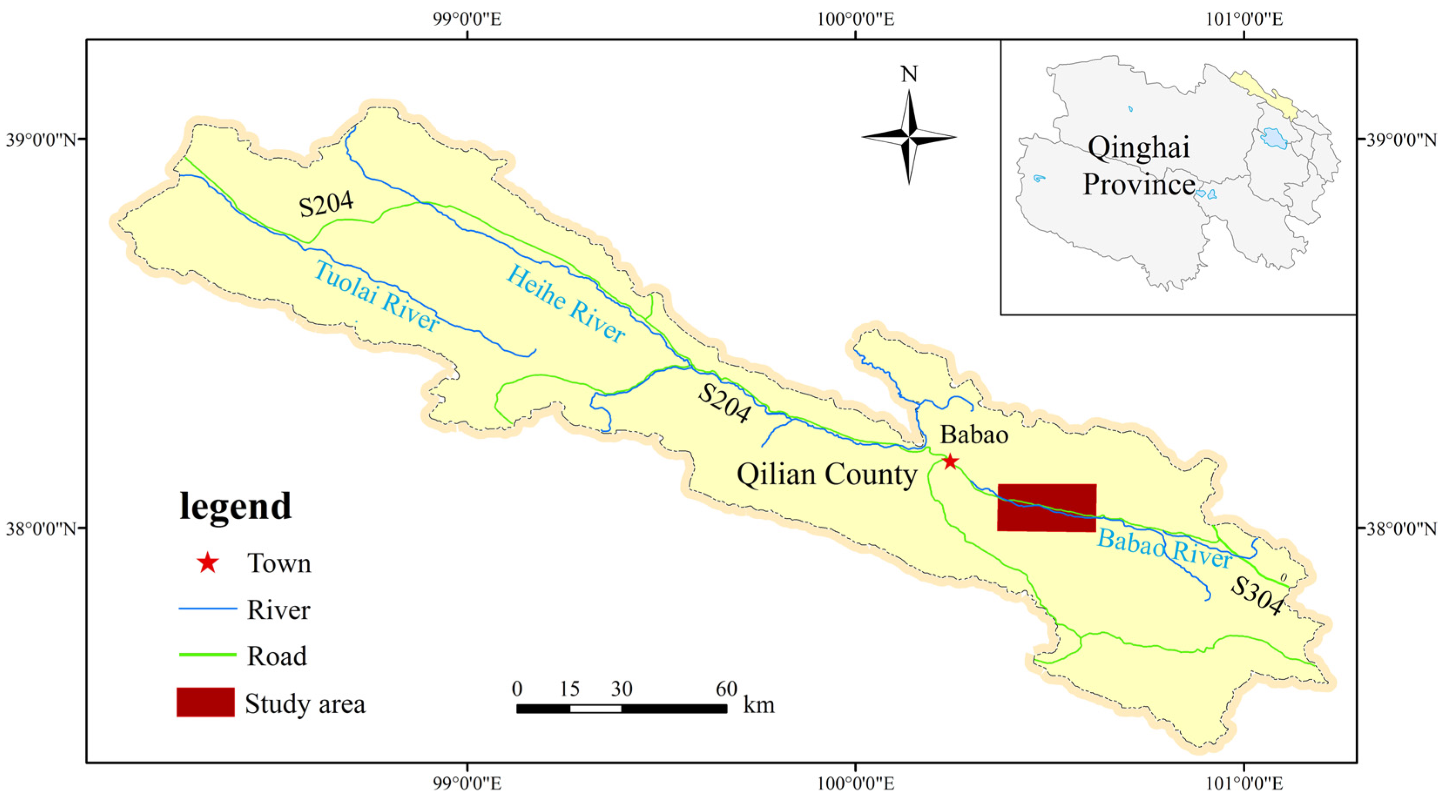
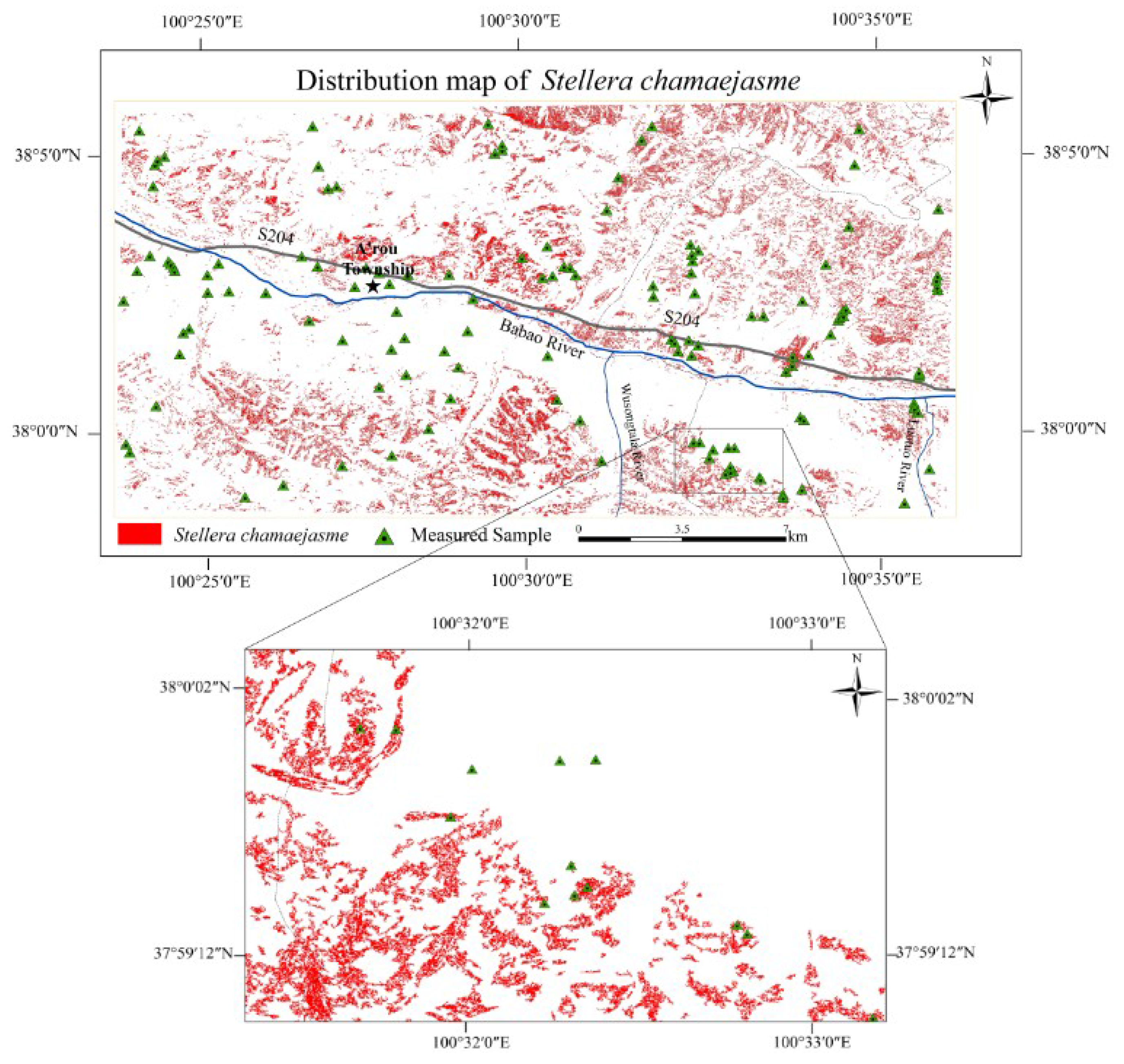
2.1. Study Area

The study area is located in Qilian County of Haibei Tibetan Autonomous Prefecture in Qinghai Province, China (37°25′16″–39°05′18″N, 98°05′35″–101°02′06″E) with an average elevation of 3000 m (Figure 1). The study area is flat and broad; the terrain gradually rises from east to west, crossed by the Babao River in the middle. It has a typical plateau continental climate characterized by long sunlight time, high daily temperature difference, and annual precipitation of 406.7 mm. The grassland type typically belongs to degenerated alpine meadow with total community coverage of 85–90%, and the grass community is richly composed of S. chamaejasme, Kobresia Willd, Oxytropis falcata Bge, Potentilla freyniana Bornm, Leymus secalinus (Georgi) Tzvel., Poa pratensis, etc. The region was originally natural grassland dominated by tussock grass; the area of S. chamaejasme has been significantly increased due to long-term overgrazing, thus forming a degenerated meadow with patchy and clumped distribution of S. chamaejasme communities with the maximum coverage about 70%. According to “Control Plan for the Toxic Grasses of Qilian County in 2011” [44], S. chamaejasme has been widespread in many towns, such as Ebao, Mole, Arou, and Yeniugou, and the damaged area is 9.03 × 10⁴ hm2, which accounts for 8.98% of the total grassland area in Qilian County.
Figure 1. Study area located in Qilian County of Qinghai Province, China.
Remotesensing 08 00148 g001

2.2. Field Spectra Measurements

Field spectral data were acquired by AvaField–1 spectroradiometer (Avantes, Apeldoorn, The Netherlands). The parameters of the spectroradiometer include spectral range of 200–1100 nm, spectrum sampling interval of 0.6 nm, wavelength precision of ±0.1 nm, and fore optic of 25° [45].
In order to analyze the spectral difference between S. chamaejasme and surrounding pasture grasses, the field measured spectra were collected in the full-bloom stage of the toxic grass, mainly including: spectra of the white flowers and leaves of S. chamaejasme, spectra of leaves of the major pasture grasses (Kobresia Willd, Oxytropis falcata Bge, Leymus secalinus (Georgi) Tzvel., Potentilla freyniana Bornm, and Poa pratensis), and spectra of S. chamaejasme communities with different coverage and the pasture grass communities. White flowers, leaves of S. chamaejasme, and leaves of major pasture grasses were bundled in situ measurement; the spectroradiometer probe was vertical and 5 cm away from the bundle. In order to avoid ambient interference, only chaplets and leaves should be maintained in the field of view. Ten spectra were acquired for each measurement and each sample was arranged in triplicate; the averaged measurement was used as the reflectance spectrum of the sample. The quadrats (1 m × 1 m) of S. chamaejasme communities with different coverage and the pasture communities were arranged in the spectra tested site; the pasture communities were evenly distributed with average coverage of 85%. The probe was positioned 2.2 m above the measured quadrat, which resulted in a 1-m diameter field of view for the measurement. The mixed reflectance spectra of S. chamaejasme-grass-soil and grass-soil were acquired [45,46].

2.3. Remote Sensing Data

The full-bloom stage of S. chamaejasme in the study area is from about 5 to 20 July. In order to explore the applicability of high resolution multispectral satellite images for S. chamaejasme recognition, IKONOS multispectral image acquired on 7 July 2011 were chosen as original data. IKONOS image were acquired by the satellite of Space Imaging Company, which was launched on 24 September 1999, with 681 km sun-synchronous polar-circular orbit, 11 days of revisit period, and swath width of 11 km. The image includes four multispectral bands and one panchromatic band and the gray level is 2048 (11 bits). Table 1 shows band information for the IKONOS image [43,47].
Table 1. Bands included in IKONOS image.
BandsSpectral Interval (nm)Spatial Resolution (m)Grayscale of Data (bits)
Blue band450–525411
Green band510–600411
Red band630–700411
Near-infrared band760–850411
Panchromatic band450–900111

2.4. Methodology

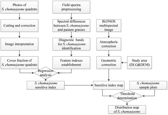
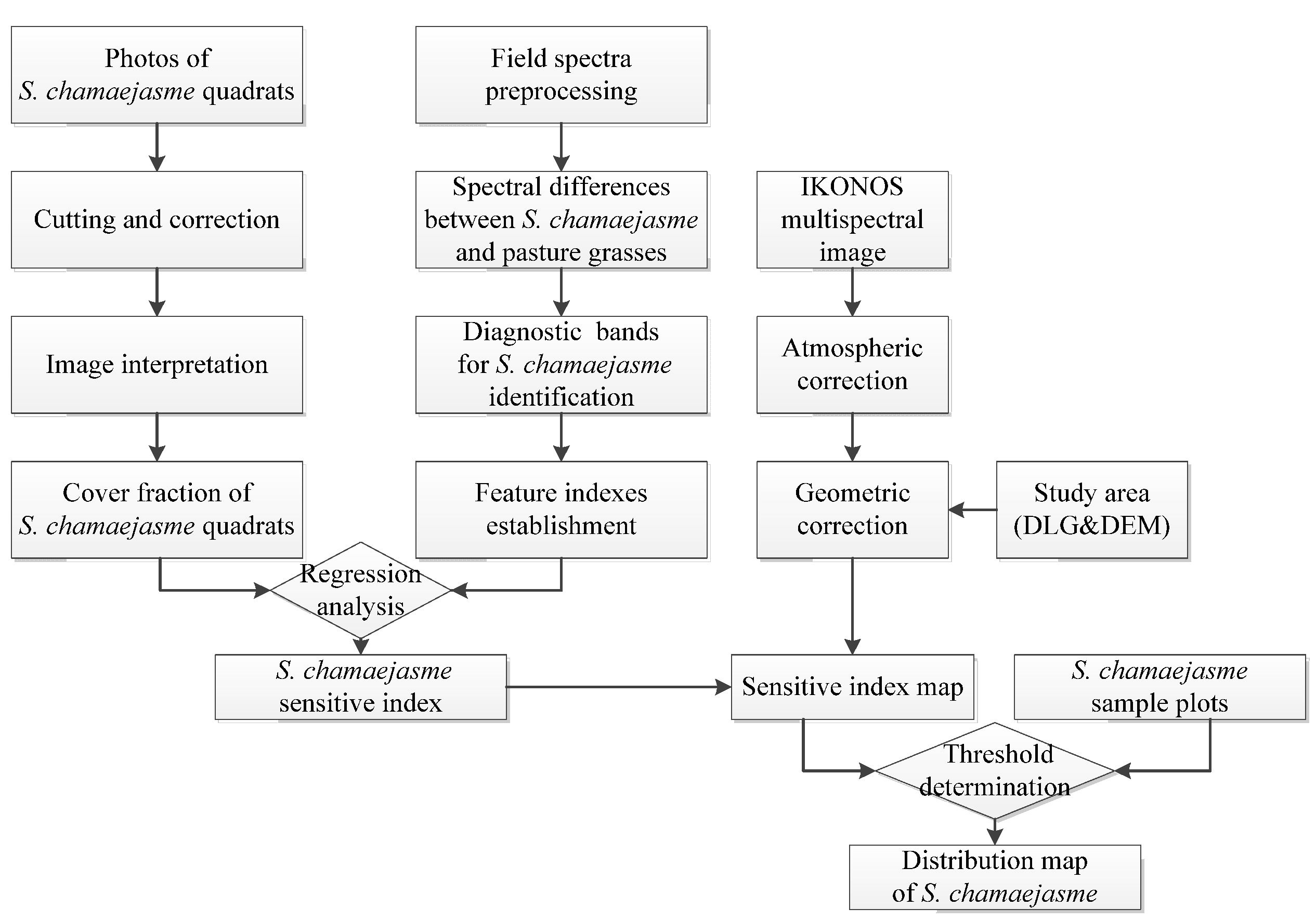
2.4.1. Overview of Methodology

The basic methodology in the study is introduced as follows (Figure 2): Firstly, the spectral differences between S. chamaejasme in the full-bloom stage and other pasture grasses were analyzed by measured spectra data and the diagnostic bands of S. chamaejasme recognition were determined. Secondly, according to the ratio and normalization principle, several indexes related to characteristics of S. chamaejasme were constructed with corresponding IKONOS bands. Thirdly, the actual cover fraction of S. chamaejasme quadrats were interpreted using the coverage photos of quadrats, and the indexes were derived from the measured quadrats spectra. The linear regression analysis between the indexes and cover fractions was performed to obtained S. chamaejasme sensitive index. Then, a S. chamaejasme sensitive index map of the study area was derived based on IKONOS multispectral image; corresponding pixels of S. chamaejasme sample plots with different coverage were identified on the map using GPS coordinates. The threshold range for S. chamaejasme distribution was determined by the sensitive index value of these pixels, and the distribution area of S. chamaejasme was extracted using the thresholding approach. Finally, the result was verified with the field measurements.
Figure 2. Flow chart of the methodology.
Remotesensing 08 00148 g002

2.4.2. Coverage Interpretation of S. Chamaejasme Quadrats

We randomly selected 38 quadrats of the S. chamaejasme communities with different coverage in the spectra tested site and simultaneously vertically photographed each quadrat. After cutting and geometric correction, the actual cover fraction of S. chamaejasme community quadrat was interpreted according to the grid method [19,48,49]. The estimated coverage is the inscribed circle area of the quadrat due to the fact that the field of view for spectral measurement is a circle with a diameter of 1 m (Figure 3).
Figure 3. Coverage Interpretation of S. chamaejasme quadrat (a) original quadrat photo, (b) photo after cutting and correction, (c) coverage interpretation.
Remotesensing 08 00148 g003

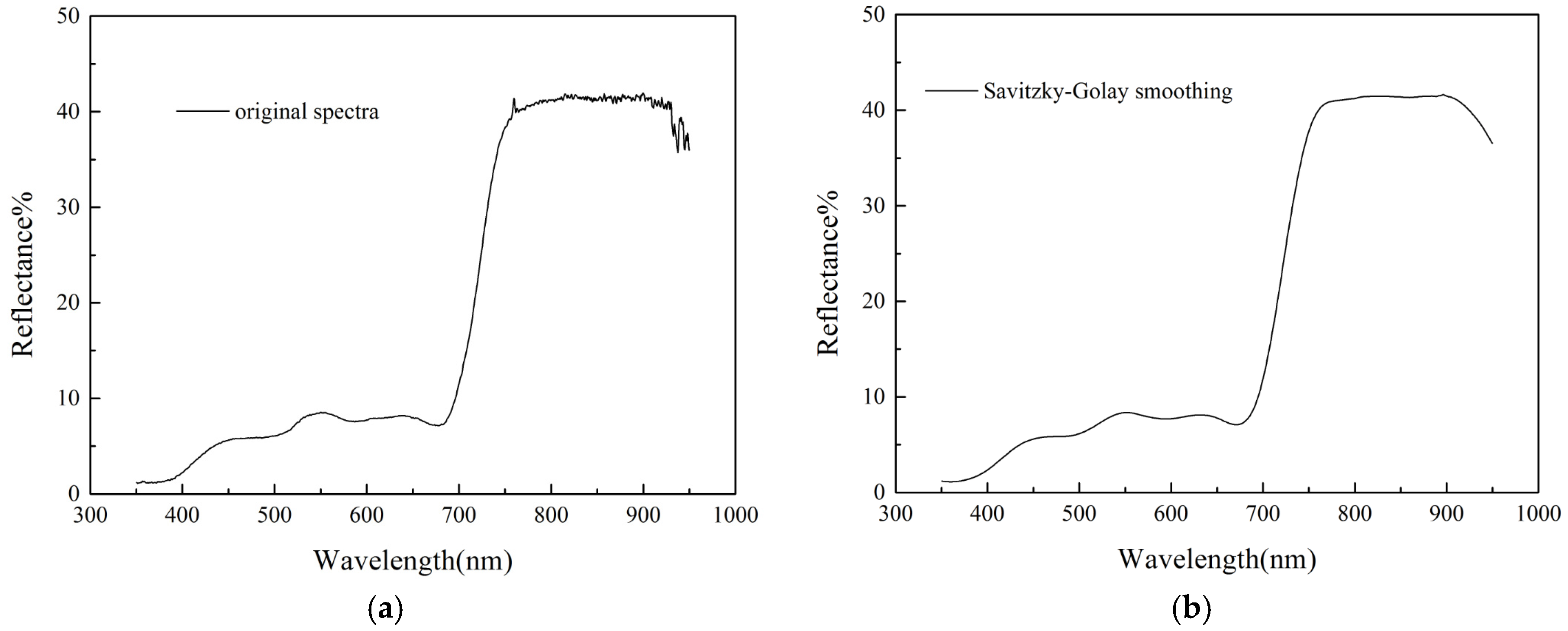
2.4.3. Spectra Data Preprocessing

The spectral band within 350–900 nm were selected as the effective data according to the spectroradiometer measurement range, then the noises existed in the original spectra was removed with a window-moving polynomial-fitting smoothing approach (Savitzky–Golay) [50]. Using this approach, polynomial fitting was performed with the data points included in each window based on the least squares principle and then the curve was smoothed by continually moving the window. Figure 4a,b display the original and smoothed spectra, respectively. The results indicated that the approach could retain the detailed reflection and absorption features in the spectral curve while suppressing the noise.
Figure 4. Spectral curve smoothing based on the Savitzky–Golay approach. (a) Original spectral curve; (b) smoothed spectral curve.
Remotesensing 08 00148 g004

2.4.4. Remote Sensing Data Preprocessing

The four IKONOS multispectral bands were firstly atmospherically corrected based on the FLAASH model [51,52], then topographically corrected by a normalization method [53]. That is, the terrain shadow was calculated using parameters, such as sun elevation and sun azimuth, combined with the DEM data; the correction factor was determined based on the shadow and each band was corrected on a pixel-by-pixel basis. Finally, integrated with GPS points and DLG and DEM datasets, the geometric correction was performed using the second-order polynomial model and applied previously rectified image as reference data [54,55]. The error was controlled to within an half of pixel to ensure that the GPS points precisely coincided with corresponding ground sites.

2.4.5. Feature Indexes Construction Based on IKONOS Image

Vegetation indexes were constructed with various combinations based on remote sensing bands to highlight vegetation characteristics or details, and provided a basis for the identification of different vegetation types [56]. In this paper, followed by the principles of the ratio vegetation index (RVI) [57] and the normalized difference vegetation index (NDVI) [57], the feature indexes related to S. chamaejasme were constructed with the IKONOS multispectral bands, which corresponded to the diagnostic spectral bands for S. chamaejasme extraction.

3. Results and Discussion

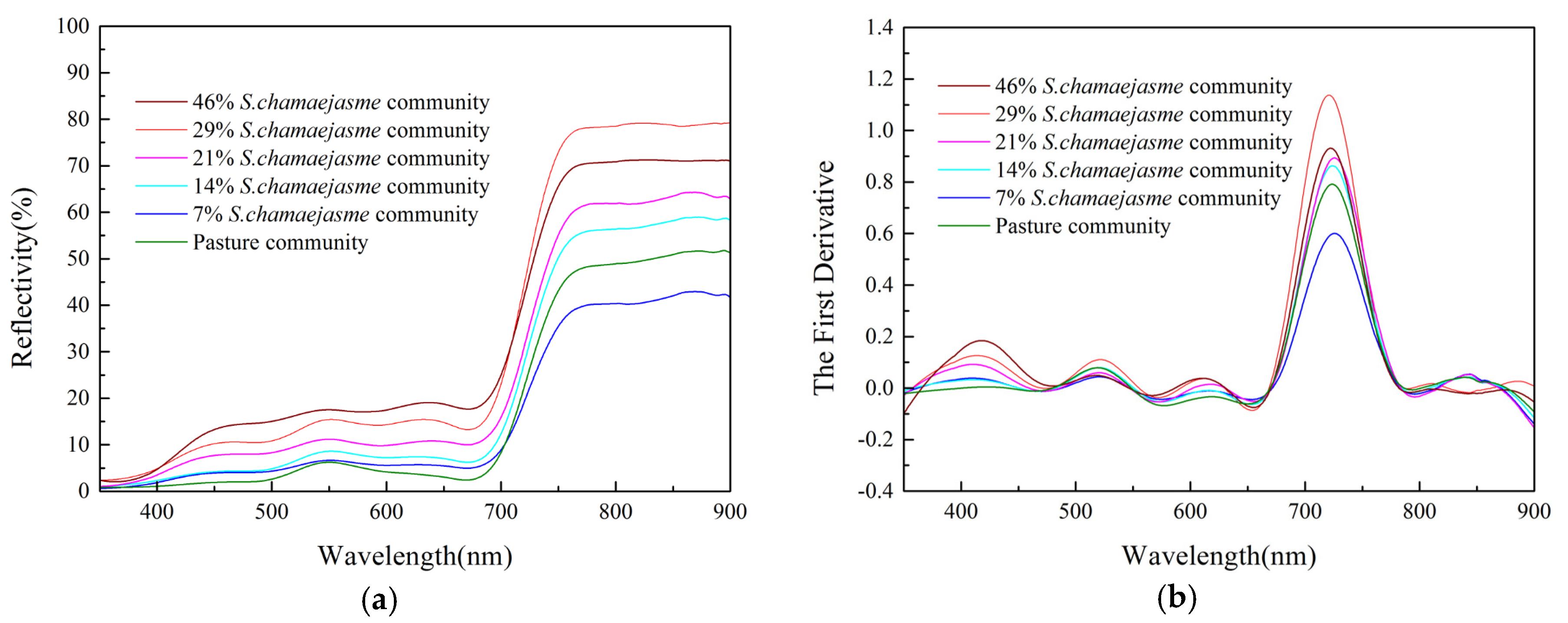
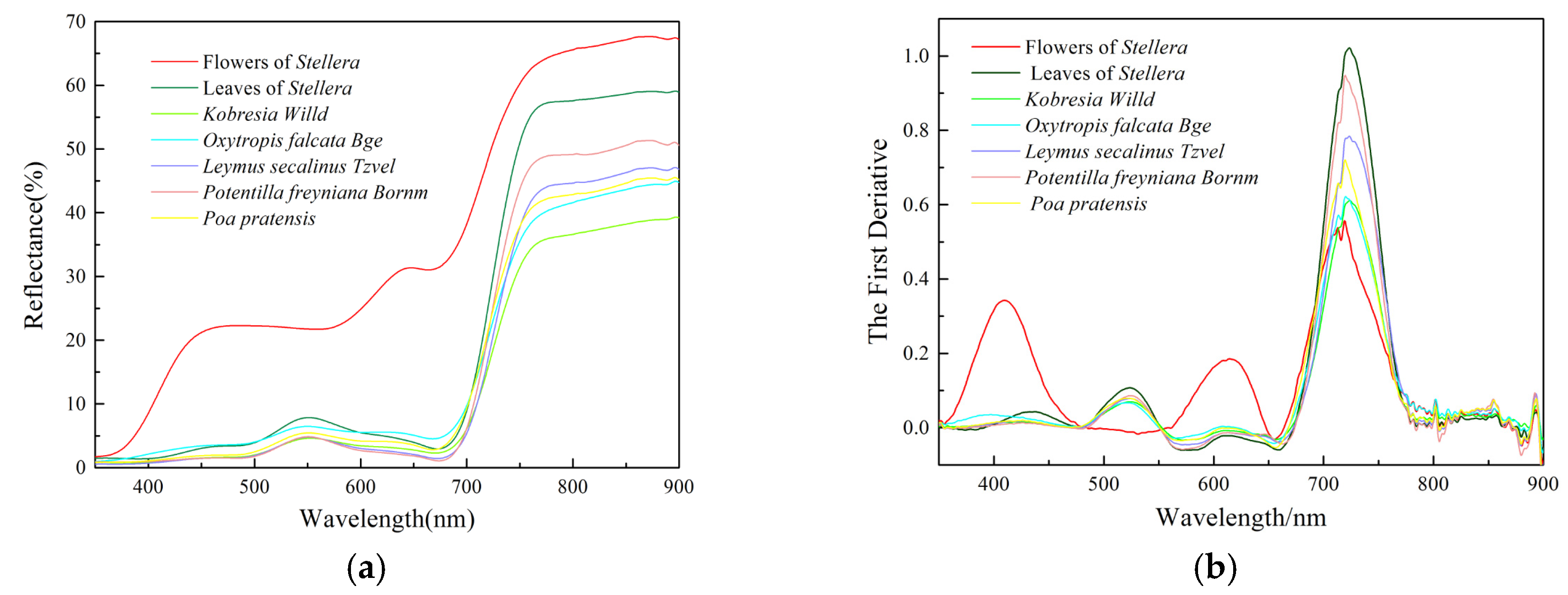
3.1. Spectral Differences between S. Chamaejasme and Surrounding Pasture Grasses

The terminal flowers of S. chamaejasme were purple in the bud stage and white in the blooming stage. The distribution of S. chamaejasme communities in the full-bloom stage shows the large-area, high-coverage, and patchy aggregation pattern. The distant view (Figure 5) presents an obvious pink-white halo, which is significantly different from the surrounding green pasture. The pasture grasses in the same blooming stage with S. chamaejasme mainly include Potentilla freyniana Bornm and Oxytropis falcata Bge, which have yellow and purple flowers, respectively; these flowers are small and sparsely distributed, with a less than 2% proportion in the distribution area of S. chamaejasme, so the two species hardly contributed to the white color in the region. Therefore, the remarkable spectral characteristics of terminal flowers provide the basis for S. chamaejasme recognition.
Figure 5. Distribution of the S. chamaejasme community in the study area, in Baishiya Village, Ebao Town, Qilian County, China (38°02′33.77″N, 100°32′01.82″E). The average coverage of the S. chamaejasme community in an alpine meadow is about 60%.
Remotesensing 08 00148 g005
Figure 6a presents the reflectance spectra curves of the white flowers, leaves of S. chamaejasme, and leaves of pasture grasses. In the wavelength range of 350–900 nm, the reflectance of white flowers of S. chamaejasme is obviously higher than that of the leaves of S. chamaejasme and pasture grasses, and present a fluctuating upward trend, while the reflectance spectra of the leaves of S. chamaejasme and pasture grasses show the typical spectral features of green plants, including a reflectance peak of 10% at 550 nm, an obvious absorption valley at 675 nm, and a steep increase with a highest reflectance of more than 60% in the near-infrared region of 700–750 nm. Due to the difference in the chlorophyll content and cell structure, the spectra of leaves of different species show a weak difference in the range of 350–700 nm and a significant difference in the range of 700–900 nm. The reflectance of leaves of S. chamaejasme is higher than that of the leaves of other pasture grasses.
Figure 6. Reflectance spectra (a) and first-order differential spectra (b) of the white flowers, leaves of S. chamaejasme, and leaves of pasture grasses.
Remotesensing 08 00148 g006
To further study the spectral differences between S. chamaejasme and pasture grasses, we adopted the related feature parameters of reflectance spectra and the first-order differential spectra (Table 2) in the subsequent analysis [58,59]. As shown in Figure 6a, the most significant reflectance differences between the white flowers of S. chamaejasme and the green background (including leaves of S. chamaejasme and pasture grasses) were observed at the red valley, followed by the blue valley. The first-order differential spectra highlighted the spectral change features of various targets. As shown in Figure 6b, in the range from 350 to 650 nm, the first-order differential spectra of white flowers of S. chamaejasme show the opposite spectral features to that of the green background. The significant difference between them was yellow edge amplitude, followed by blue edge amplitude. Although the most significant difference in the first-order differential spectra between the two was observed in the range from 350 nm to 450 nm, there is no further discussion because corresponding remote sensing bands were not available. Taking into account IKONOS multispectral bands, the red and blue bands showed the remarkable spectral difference between white flowers of S. chamaejasme and the green background.
Table 2. Definitions of spectral feature parameters.
Spectral Feature ParametersDefinitions
Blue edge amplitudeThe maximum first-order differential reflectance of blue edge band between 490 and 530 nm
Yellow edge amplitudeThe maximum first-order differential reflectance of yellow edge band between 560 and 640 nm
Red edge amplitudeThe maximum first-order differential reflectance of red edge band between 680 and 760 nm
Blue valleyThe minimum reflectance of blue band between 450 and 515 nm
Green peakThe maximum reflectance of green band between 510 and 560 nm
Red valleyThe minimum reflectance of red band between 640 and 680 nm
Near-infrared peakThe maximum reflectance of near-infrared band between 780 and 900 nm
Each pixel value of remote sensing images represents the mixed spectral information of all the ground objects in the corresponding area. For S. chamaejasme communities, the pixel value represents the mixed spectral information of S. chamaejasme, pasture, and soil. The field measured spectra shown in Figure 7a indicated that the spectral curves of S. chamaejasme communities with different coverage were similar in the range of 350–900 nm. With the coverage increasing of S. chamaejasme community, the reflectance gradually rises and the spectral features of white flowers become obvious. However, a weak green peak is still observed at 550 nm. In the wavelength range of 350–700 nm, the reflectance of S. chamaejasme communities with different coverage is higher than that of the pasture community. However, in the wavelength range of 700–900 nm, the reflectance of S. chamaejasme community with the lower coverage 7% is below that of the pasture community; the spectral curves of S. chamaejasme communities with coverage of 7% and 14% are similar and close to the pasture community. The spectral difference between S. chamaejasme communities with the coverage higher than 21% and the pasture community gradually increases. The most obvious difference between S. chamaejasme communities with different coverage and pasture community appears in near-infrared peak, which corresponds to the near infrared band of IKONOS image. The first-order derivative spectra curves (Figure 7b) indicate that the remarkable difference between the two is red edge amplitudes, but no regular changes.
Figure 7. Reflection spectra (a) and the first-order differential spectra (b) of the S. chamaejasme communities with different coverage and pasture community.
Remotesensing 08 00148 g007
The correlation analysis results between the spectral reflectance and the coverage of S. chamaejasme community quadrats (Figure 8) indicated that the maximum correlation coefficient R was 0.44 at 480 nm within the blue band. Another peak at 668 nm was located within the red band with R of 0.377. The correlation coefficient was relatively low and didn’t reach the significant level of 0.05 within the near-infrared band. In general, the coefficients within the band of 422–506 nm reached the significant level of 0.01 and the coefficients within the band of 611–692 nm reached the significant level of 0.05. The two ranges respectively corresponded to the blue band and red band of IKONOS images, which show good correlation between the spectral reflectance and the coverage of S. chamaejasme communities.
In conclusion, among IKONOS multispectral bands, the red band and blue band show the spectral difference between the white flowers of S. chamaejasme and the green background. Moreover, the reflectance of the two bands was significantly correlated with the coverage of S. chamaejasme communities. The near-infrared band represented the spectral difference among the S. chamaejasme communities with different coverage, and the difference between S. chamaejasme communities and pasture communities. The three bands can be used as the diagnostic bands for S. chamaejasme classification.
Figure 8. Correlation analysis between the spectral reflectance and coverage of S. chamaejasme community quadrats.
Remotesensing 08 00148 g008

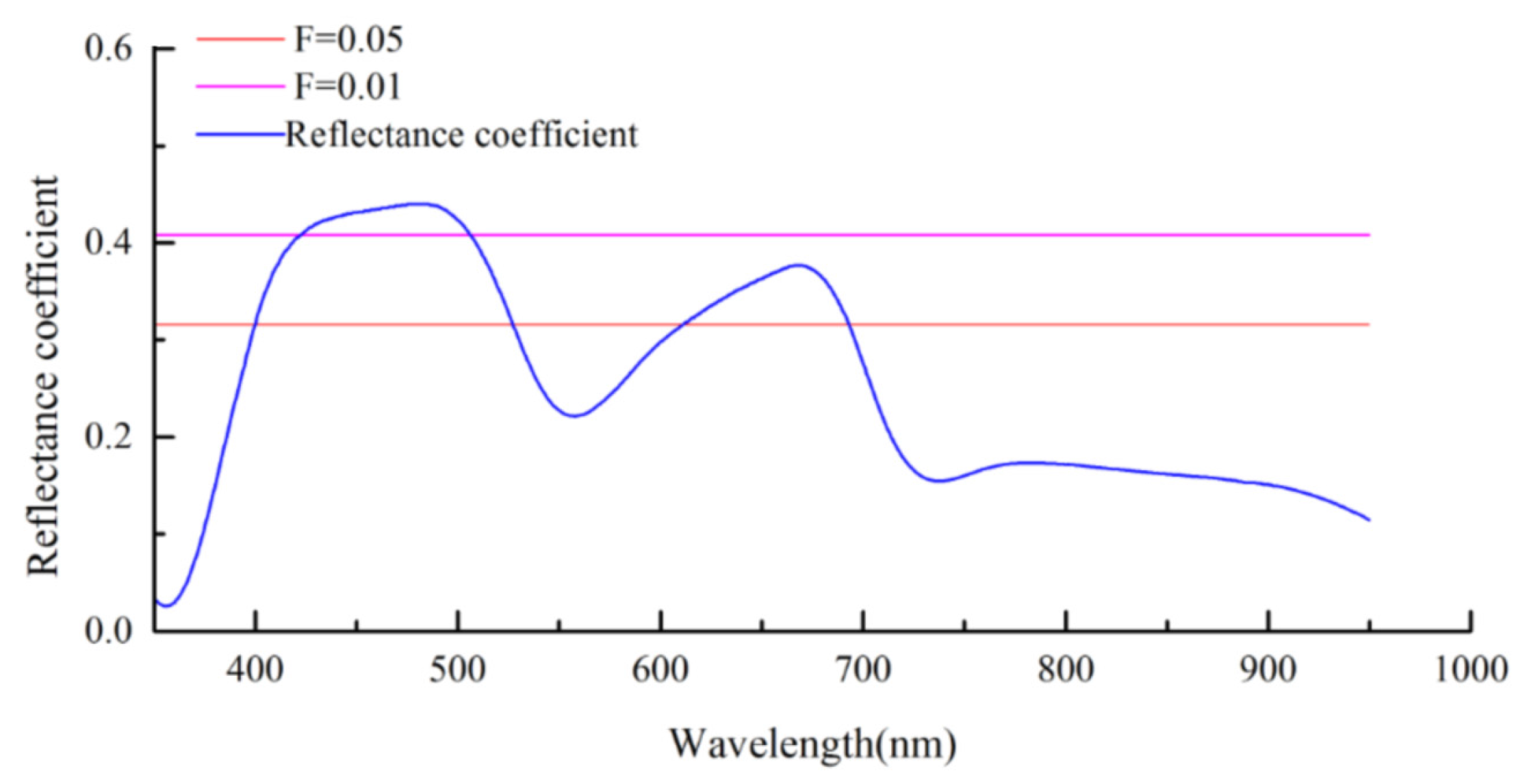
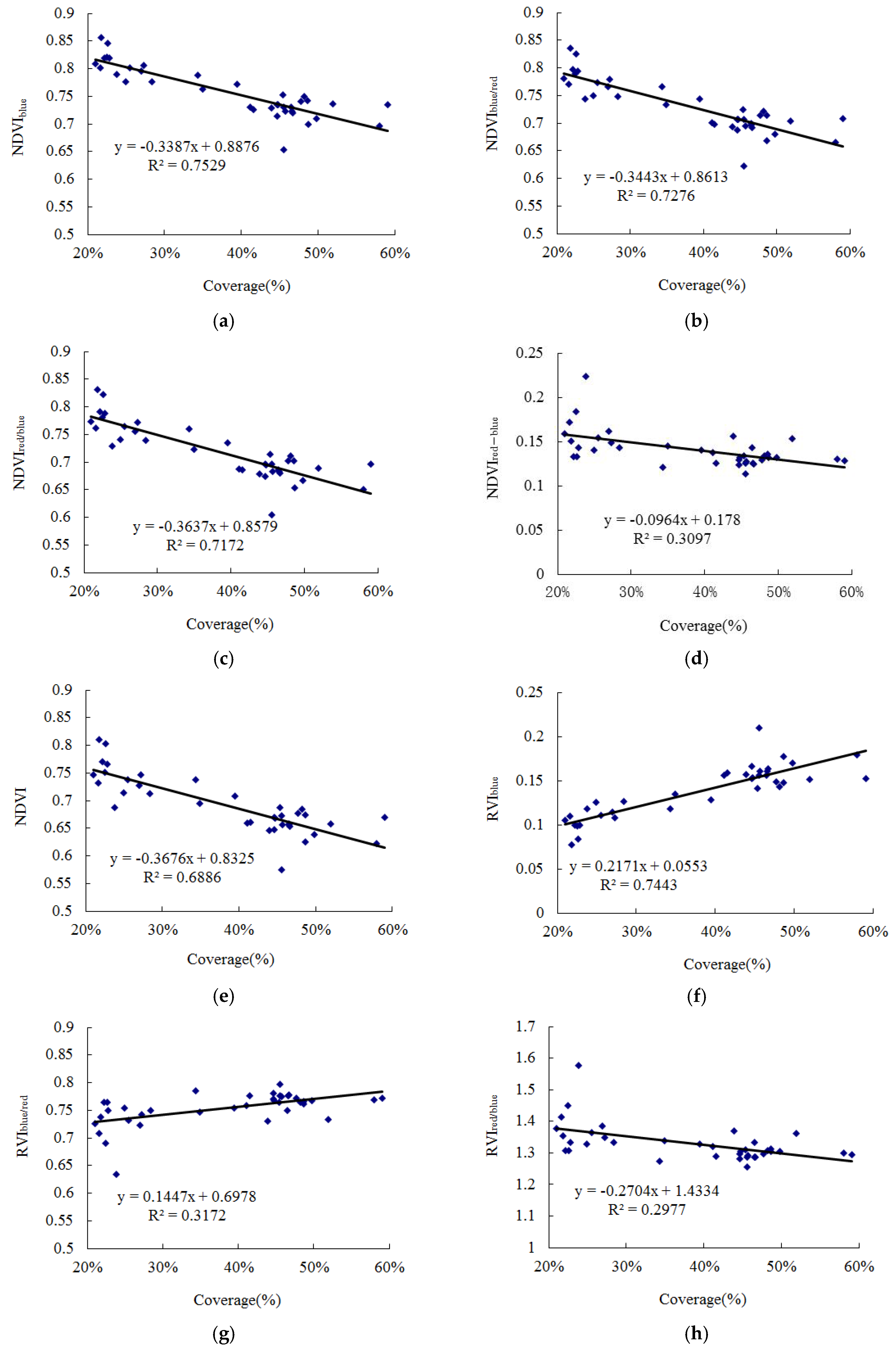
3.2. Sensitive Index Analysis

The above spectral analysis of S. chamaejasme and pasture grasses indicated that the full-bloom stage was the optimal time for S. chamaejasme recognition. With the blue, red, and near-infrared bands of IKONOS images, various indexes highlighting the features of S. chamaejasme were established as follows:
N D V I b l u e = ρ n i r ρ b l u e ρ n i r + ρ b l u e
N D V I b l u e / r e d = ρ n i r ρ b l u e ρ n i r + ρ r e d
N D V I r e d / b l u e = ρ n i r ρ r e d ρ n i r + ρ b l u e
N D V I r e d b l u e = ρ r e d ρ b l u e ρ r e d + ρ b l u e
N D V I = ρ n i r ρ r e d ρ n i r + ρ r e d
R V I b l u e = ρ b l u e ρ n i r
R V I b l u e / r e d = ρ b l u e ρ r e d
R V I r e d / b l u e = ρ r e d ρ b l u e
R V I = ρ r e d ρ n i r
where ρ n i r , ρ r e d , and ρ b l u e are denoted as the reflectance within the near-infrared, red, and blue bands of IKONOS image, respectively.
The remote sensing image pixels indicated the spectra information of S. chamaejasme communities with different coverage. Therefore, we performed the linear regression analysis between coverage of S. chamaejasme community and individual index to determine S. chamaejasme sensitive index. Seven indexes, NDVI, and RVI were derived from field quadrat spectra, the analysis (Figure 9) showed good results for N D V I b l u e , N D V I b l u e / r e d , N D V I r e d / b l u e , and R V I b l u e with the coefficient of determination R2 value above 0.7. Among all the indexes, N D V I b l u e presented the highest coefficient of determination R2 value of 0.7529 and could be taken as the sensitive index for distribution extraction of S. chamaejasme.
Figure 9. Linear regression analysis between coverage of S. chamaejasme community and feature indexes (n = 38). (ai) Corresponds to the indexes in Equations (1)–(9).
Remotesensing 08 00148 g009aRemotesensing 08 00148 g009b

3.3. Distribution Extraction of S. chamaejasme
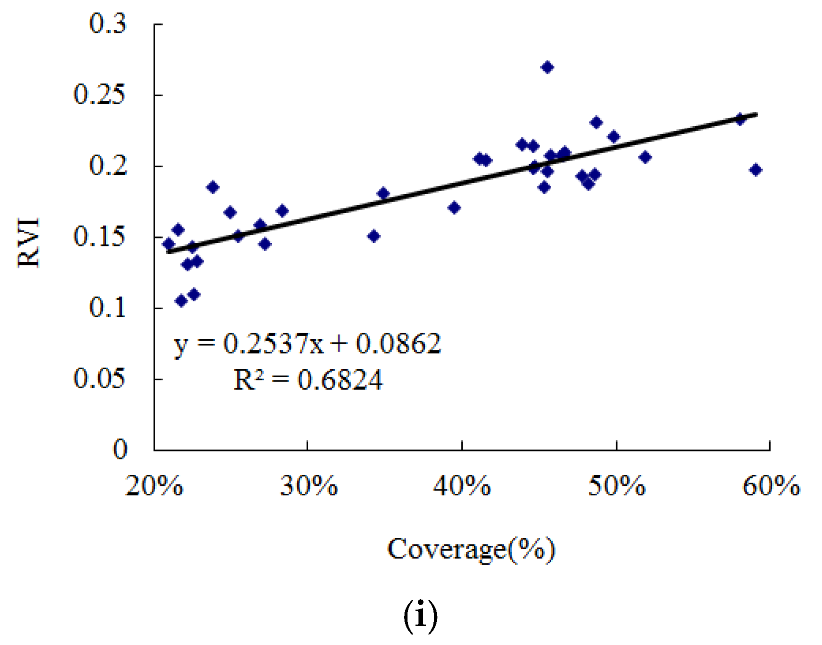
The sensitive index map based N D V I b l u e was calculated by IKONOS multispectral image using Equation (1). Thirty sampling plots were selected according to coverage characteristics of S. chamaejasme communities in the study area. The pixels on the sensitive index map corresponding to the plots of S. chamaejasme communities with different coverage were identified by GPS coordinates. Then, according to the N D V I b l u e values of these pixels, we determined the threshold range for S. chamaejasme distribution was 0.40–0.43. The distribution area of S. chamaejasme was initially extracted by the thresholding approach. Since the image spectra of bare soil, rocks, and snow cover were similar to that of S. chamaejasme, some pixels were prone to be misclassified. Combined with the aspect dataset, the mixed pixels were further eliminated in terms of environmental properties of S. chamaejasme, and the distribution area of S. chamaejasme was finally derived as shown in Figure 10.
Figure 10. Distribution map of S. chamaejasme in the study area.
Remotesensing 08 00148 g010

3.4. Validation

3.4.1. Statistical Data Validation

According to the statistical data in “Control Plan for the Toxic Grasses of Qilian County in 2011” [44], the area damaged by S. chamaejasme in Qilian County is 9.03 × 10⁴ hm2 in 2011 and accounts for 8.98% of the total grassland area in the county. The distribution area of S. chamaejasme extracted based on the IKONOS image is 2614.93 ha, which accounted for 9.42% of the total grassland area (27,755.2 ha) in the study region. Therefore, the remote sensing based distribution extraction of S. chamaejasme was basically consistent with the actual situation.

3.4.2. Field Data Validation

Field tested points were randomly selected in the study area to verify the extracted result, including 91 points in S. chamaejasme distribution area and 49 points in farmland and grassland (Figure 10). The Kappa coefficient, user accuracy, and overall accuracy [60] are 0.80, 89.01%, and 90.71%, respectively (Table 3 and Table 4). The classification error matrix indicated that the 10 points misclassified as S. chamaejasme were distributed on the sides of roads and rivers, as well as on shaded hills. The mistaken classification therefore might be caused by human activities, river interference, or shadows. The validation indicated that the proposed method could obtain good accuracy in S. chamaejasme distribution extraction on a large scale.
Table 3. Classification error matrix.
IField Tested Results
J S. chamaejasmeFarmland/GrasslandTotal
Classified resultsS. chamaejasme811091
Farmland/grassland34649
Total8455140
Table 4. Classification accuracy evaluation.
CategoriesMapping Accuracy (%)User Accuracy (%)
S. chamaejasme96.4389.01
Farmland/grassland82.1493.88
Overall accuracy = 90.71%Kappa coefficient = 0.80

4. Conclusions

The particular spatial pattern of S. chamaejasme communities and the significant difference between white flowers of S. chamaejasme and the green background provide the basis for remote sensing distribution monitoring of S. chamaejasme.
The spectral difference analysis between S. chamaejasme and pasture grasses demonstrated that the red, blue, and near-infrared bands of IKONOS image could be used as the diagnostic bands for S. chamaejasme recognition. The linear regression analysis between the coverage of S. chamaejasme communities and feature indexes showed best result for N D V I b l u e with the R2 value above 0.7529. Distribution area of the S. chamaejasme was extracted in the study area with the sensitive index of N D V I b l u e based on IKONOS multispectral image. The validation indicated that the user accuracy and overall accuracy were 89.01% and 90.71%, respectively. Although existing aerial and satellite hyperspectral images hardly met the dynamic monitoring of toxic grasses, high resolution multispectral satellite images (IKONOS image) showed the significant application advantages in toxic grasses recognition. The study is of great significance to grassland management and livestock production.
With the coverage decreasing of the S. chamaejasme community, the proportion of white flowers of S. chamaejasme decreases and the proportion of green background increases. Therefore, the spectral characteristics of S. chamaejasme community with low coverage become close to the pasture community, thus leading to a decline in the recognition accuracy of S. chamaejasme. With the coverage increasing of the S. chamaejasme community, the spectral differences between the S. chamaejasme community and the pasture community become significant and the two can be differentiated by using the N D V I b l u e index. Integrated with field investigation results, we considered that it was difficult to distinguish S. chamaejasme communities with coverage lower than 20% from the pasture community. Determination and validation of community coverage threshold are underway for identifying S. chamaejasme based on remote sensing data.

Acknowledgments

The study was supported by the Ministry of Agriculture’s Special Funds for Scientific Study on Public Causes (Grant No. 201203062) and the National Science Foundation of China (Grant No. 41171225).

Author Contributions

Yongmei Liu conceived and designed the experiments; Jingzhong Li, Lei Wang and Guowei Pang performed the experiments; Jingzhong Li analyzed the data; Chonghui Mo and Mingming Cao contributed reagents/materials/analysis tools; Jingzhong Li and Yongmei Liu wrote the paper.

Conflicts of Interest

The authors declare no conflict of interest.

References

  1. Scurlock, J.M.O.; Johnson, K.; Olson, R.J. Estimating net primary productivity from grassland biomass dynamics measurements. Glob. Change Biol. 2002, 8, 736–753. [Google Scholar] [CrossRef]
  2. Wu, C.; Wang, W.; Liu, X.; Ma, F.; Cao, D.; Yang, X.; Wang, S.; Geng, P.; Lu, H.; Zhao, B. Pathogenesis and preventive treatment for animal disease due to locoweed poisoning. Environ. Toxicol. Pharmacol. 2014, 37, 336–347. [Google Scholar]
  3. Zhao, B.; Liu, Z.; Lu, H.; Wang, Z.; Sun, L.; Wan, X.; Guo, X.; Zhao, Y.; Wang, J.; Shi, Z. Damage and control of poisonous weeds in western grassland of China. Agric. Sci. China 2010, 10, 1512–1521. [Google Scholar] [CrossRef]
  4. Wen, L.; Dong, S.K.; Zhu, L.; Li, X.Y.; Shi, J.J.; Wang, Y.L.; Ma, Y.S. The construction of grassland degradation index for alpine meadow in Qinghai-Tibetan Plateau. Procedia Environ. Sci. 2010, 2, 1966–1969. [Google Scholar] [CrossRef]
  5. Zhang, Y.S.; Zhao, X.Q.; Zhou, X.M. Strategy and countermeasure for sustainable development of animal husbandry in Qinghai. J. Nat. Resour. 2000, 4, 328–334. (In Chinese) [Google Scholar]
  6. Wei, Y.; Wang, L.; Shi, Y.; Li, L. Net productivity of grassland resources monitoring based on remote sensing data in Qinghai Province. Sci. Geogr. Sin. 2012, 5, 621–627. (In Chinese) [Google Scholar]
  7. Harris, R.B. Rangeland degradation on the Qinghai-Tibetan plateau: A review of the evidence of its magnitude and causes. J. Arid Environ. 2010, 74, 1–12. [Google Scholar] [CrossRef]
  8. Wen, L.; Dong, S.K.; Li, Y.Y. The effects of biotic and abiotic factors on the spatial heterogeneity of alpine grassland vegetation at a small scale on the Qinghai-Tihet Plateau, China. Environ. Monit. Assess. 2013, 10, 8051–8064. [Google Scholar] [CrossRef] [PubMed]
  9. Goslee, S.C.; Peters, D.P.C.; Beck, K.G. Modeling invasive weeds in grasslands: The role of allelopathy in Acroptilon repens invasion. Ecol. Model. 2001, 139, 21–45. [Google Scholar] [CrossRef]
  10. Zhao, M.; Gao, X.; Wang, J.; He, X.; Han, B. A review of the most economically important poisonous plants to the livestock industry on temperate grasslands of China. J. Appl. Toxicol. 2013, 33, 9–17. [Google Scholar] [CrossRef] [PubMed]
  11. Yan, Z.; Guo, H.; Yang, J.; Liu, Q.; Jin, H.; Xu, R.; Cui, H.; Qin, B. Phytotoxic flavonoids from roots of S. chamaejasme L. (Thymelaeaceae). Phytochemistry 2014, 106, 61–68. [Google Scholar] [CrossRef] [PubMed]
  12. Shi, Z.C. The Poisonous Plants of Chinese Grassland, 1st ed.; China Agriculture Press: Beijing, China, 1997. (In Chinese) [Google Scholar]
  13. Sun, G.; Luo, P.; Qiu, P.F.; Gao, Y.H.; Chen, H.; Shi, F.S. S. chamaejasme L. increases soil N availability, turnover rates and microbial biomass in an alpine meadow ecosystem on the eastern Tibetan Plateau of China. Soil Biol. Biochem. 2009, 41, 86–91. [Google Scholar] [CrossRef]
  14. Zhang, Y.H.; Volis, S.; Sun, H. Chloroplast phylogeny and phylogeography of S. chamaejasme on the Qinghai-Tibet Plateau and in adjacent regions. Mol. Phylogenet. Evol. 2010, 57, 1162–1172. [Google Scholar] [CrossRef] [PubMed]
  15. Zhang, G.Z.; Chen, Y.L.; Wang, Y.W.; Xiu, H.H. S. chamaejasme L. an pesticide plant of Thymelaeaceae. J. Cent. China Norm. Univ. 2000, 3, 326–330. (In Chinese) [Google Scholar]
  16. Lu, H.; Wang, S.S.; Zhou, Q.W.; Zhao, Y.N.; Zhao, B.Y. Damage and control of major poisonous plants in the western grasslands of China—A review. Rangel. J. 2012, 34, 329–339. [Google Scholar] [CrossRef]
  17. Gao, F.; Zhao, C.; Shi, F.; Sheng, Y.; Ren, H.; He, G. Spatial pattern of S. chamaejasme population in degraded alpine grassland in northern slope of Qilian Mountains, China. Chin. J. Ecol. 2011, 6, 1312–1316. [Google Scholar]
  18. Lawrence, R.L.; Wood, S.D.; Sheley, R.L. Mapping invasive plants using hyperspectral imagery and Breiman Cutler classifications (RandomForest). Remote Sens. Environ. 2006, 100, 356–362. [Google Scholar] [CrossRef]
  19. Wang, H.; Qian, J.; Ma, M.; Wang, X. The spectral characteristics of S. chamaejasme L. with varied coverage in Qilian of China. Proc. SPIE 2009. [Google Scholar] [CrossRef]
  20. Gausman, H.W.; Menges, R.M.; Escobar, D.E.; Everitt, J.H.; Bowen, R.L. Pubescence affects spectra and imagery of Silverleaf Sunflower (Helianthus argophyllus). Weed Sci. 1977, 25, 437–440. [Google Scholar]
  21. Everitt, J.H.; Anderson, G.L.; Escobar, D.E.; Davis, M.R.; Spencer, N.R.; Andrascik, R.J. Use of remote sensing for detecting and mapping leafy spurge (Euphorbia esula). Weed Technol. 1995, 3, 599–609. [Google Scholar]
  22. Underwood, E.; Ustin, S.; DiPietro, D. Mapping nonnative plants using hyperspectral imagery. Remote Sens. Environ. 2003, 86, 150–161. [Google Scholar] [CrossRef]
  23. Miao, X.; Gong, P.; Swope, S.; Pu, R.; Carruthers, R.; Anderson, G.L.; Heaton, J.S.; Tracy, C.R. Estimation of yellow starthistle abundance through CASI-2 hyperspectral imagery using linear spectral mixture models. Remote Sens. Environ. 2006, 101, 329–341. [Google Scholar] [CrossRef]
  24. Lass, L.W.; Thill, D.C.; Shafii, B.; and Prather, T.S. Detecting spotted knapweed (Centaurea maculosa) with hyperspectral remote sensing technology. Weed Technol. 2002, 16, 426–432. [Google Scholar] [CrossRef]
  25. Mirik, M.; Ansley, R.J.; Steddom, K.; Jones, D.C.; Rush, C.M.; Michels, G.J.; Elliott, N.C. Remote distinction of a noxious weed (musk thistle: Carduus nutans) using airborne hyperspectral imagery and the support vector machine classifier. Remote Sens. 2013, 5, 612–630. [Google Scholar] [CrossRef]
  26. Williams, A.P.; Hunt, E.R. Estimation of leafy spurge cover from hyperspectral imagery using mixture tuned matched filtering. Remote Sens. Environ. 2002, 82, 446–456. [Google Scholar] [CrossRef]
  27. Lass, L.W.; Prather, T.S. Detecting the locations of Brazilian pepper trees in the everglades with a hyperspectral sensor. Weed Technol. 2004, 18, 437–442. [Google Scholar] [CrossRef]
  28. Lass, L.W.; Prather, T.S.; Glenn, N.F.; Weber, K.T.; Mundt, J.T.; Pettingill, J. A review of remote sensing of invasive weeds and example of the early detection of spotted knapweed (Centaurea maculosa) and babysbreath (Gypsophila paniculata) with a hyperspectral sensor. Weed Sci. 2005, 53, 242–251. [Google Scholar] [CrossRef]
  29. Narumalani, S.; Mishra, D.R.; Burkholder, J.; Merani, P.B.T. A comparative evaluation of ISODATA and spectral angle mapping for the detection of saltcedar using airborne hyperspectral imagery. Geocarto Int. 2006, 2, 59–66. [Google Scholar] [CrossRef]
  30. Miao, X.; Gong, P.; Swope, S.; Pu, R.; Carruthers, R.; Anderson, G.L. Detection of yellow starthistle through band selection and feature extraction from hyperspectral imagery. Photogramm. Eng. Remote Sens. 2007, 9, 1005–1015. [Google Scholar]
  31. Yang, C.; Everitt, J.H. Comparison of hyperspectral imagery with aerial photography and multispectral imagery for mapping broom snakeweed. Int. J. Remote Sens. 2010, 20, 5423–5438. [Google Scholar] [CrossRef]
  32. Evangelista, P.H.; Stohlgren, T.J.; Morisette, J.T.; Kumar, S. Mapping invasive tamarisk (Tamarix): A comparison of single-scene and time-series analyses of remotely sensed data. Remote Sens. 2009, 1, 519–533. [Google Scholar] [CrossRef]
  33. Root, R.; Tejada, P.Z.; Pinilla, C.; Ustin, S.; Kokaly, R.; Anderson, G.; Hager, S. Identification, Classification, and Mapping of Invasive Leafy Spurge Using Hyperion, AVIRIS, and CASI. Available online: http://eo1.gsfc.nasa.gov/new/validationReport/Technology/ Documents/ Tech.Val.Report/Science_Summary_Root.pdf (accessed on 25 October 2015).
  34. Wang, L.; Sousa, W.S.; Gong, P.; Biging, G.S. Comparison of IKONOS and QuickBird images for mapping mangrove species on the Caribbean coast of Panama. Remote Sens. Environ. 2004, 91, 432–440. [Google Scholar] [CrossRef]
  35. Bhaskaran, S.; Paramananda, S.; Ramnarayan, M. Per-pixel and object-oriented classification methods for mapping urban features using Ikonos satellite data. Appl. Geogr. 2010, 30, 650–665. [Google Scholar] [CrossRef]
  36. Zhou, H.; Jiang, H.; Huang, Q. Landscape and water quality change detection in urban wetland: A Post-classification comparison method with IKONOS data. Procedia Environ. Sci. 2011, 10, 1726–1731. [Google Scholar]
  37. Delm, A.V.; Gulinck, H. Classification and quantification of green in the expanding urban and semi-urban complex: Application of detailed field data and IKONOS-imagery. Ecol. Indic. 2011, 11, 52–60. [Google Scholar] [CrossRef]
  38. Pu, R.; Landry, S. A comparative analysis of high spatial resolution IKONOS and WorldView-2 imagery for mapping urban tree species. Remote Sens. Environ. 2012, 124, 516–533. [Google Scholar] [CrossRef]
  39. Laet, V.D.; Paulissen, E.; Waelkens, M. Methods for the extraction of archaeological features from very high-resolution Ikonos-2 remote sensing imagery, Hisar (southwest Turkey). J. Archaeol. Sci. 2007, 34, 830–841. [Google Scholar] [CrossRef]
  40. Malhi, Y.; María, R.; Cuesta, R. Analysis of lacunarity and scales of spatial homogeneity in IKONOS images of Amazonian tropical forest canopies. Remote Sens. Environ. 2008, 112, 2074–2087. [Google Scholar] [CrossRef]
  41. Asner, G.P.; Warner, A.S. Canopy shadow in IKONOS satellite observations of tropical forests and savannas. Remote Sens. Environ. 2003, 87, 521–533. [Google Scholar] [CrossRef]
  42. Kayitakire, F.; Hamel, C.; Defourny, P. Retrieving forest structure variables based on image texture analysis and IKONOS-2 imagery. Remote Sens. Environ. 2006, 102, 390–401. [Google Scholar] [CrossRef]
  43. Casady, G.M.; Hanley, R.S.; Seelan, S.K. Detection of Leafy Spurge using multidate high-resoultion satellite imagery. Weed Technol. 2005, 19, 462–467. [Google Scholar] [CrossRef]
  44. Qilian Grassland Station. Control Plan for the Toxic Grass of Qilian County in 2011. A government work report, unpublished. 2011. (In Chinese) [Google Scholar]
  45. Hamzeh, S.; Naseri, A.A.; Alavipanah, S.K.; Mojaradi, B.; Bartholomeus, H.M.; Clevers, J.G.P.W.; Behzad, M. Estimating salinity stress in sugarcane fields with spaceborne hyperspectral vegetation indices. Int. J. Appl. Earth Obs. Geoinform. 2013, 21, 282–290. [Google Scholar] [CrossRef]
  46. Omodanisi, E.O.; Salami, A.T. An Assessment of the spectra characteristics of vegetation in south western Nigeria. IERI Procedia 2014, 9, 26–32. [Google Scholar] [CrossRef]
  47. Yang, G.; Pu, R.; Zhao, C.; Xue, X. Estimating high spatiotemporal resolution evapotranspiration over a winter wheat field using an IKONOS image based complementary relationship and Lysimeter observations. Agric. Water Manag. 2014, 133, 34–43. [Google Scholar] [CrossRef]
  48. Chen, J.; Shen, M.; Zhu, X.; Tang, Y. Indicator of flower status derived from in situ hyperspectral measurement in an alpine meadow on the Tibetan Plateau. Ecol. Indic. 2009, 9, 818–823. [Google Scholar] [CrossRef]
  49. Daniel, G.F.; David, E.H.; Antonio, R.C.; Julian, C.; Jose, M.M.M. A digital image processing based method for determining the crop coefficient of lettuce crops in the southeast of Spain. Biosyst. Eng. 2014, 117, 23–34. [Google Scholar]
  50. Tsai, F.; Philpot, W. Derivative analysis of hyperspectral data. Remote Sens. Environ. 1998, 66, 41–51. [Google Scholar]
  51. Hanan, N.P.; Prince, S.D.; Holben, B.N. Atmospheric correction of AVHRR data for biophysical remote sensing of the Sahel. Remote Sens. Environ. 1995, 51, 306–316. [Google Scholar] [CrossRef]
  52. Magendran, T.; Sanjeevi, S. Hyperion image analysis and linear spectral unmixing to evaluate the grades of iron ores in parts of Noamundi, Eastern India. Int. J. Appl. Earth Obs. Geoinform. 2014, 26, 413–426. [Google Scholar] [CrossRef]
  53. Law, K.H.; Nichol, J. Topographic correction for differential illumination effects on IKONOS satellite imagery. Int. Arch. Photogramm. Remote Sens. Spat. Inform. Sci. 2004, 35, 641–646. [Google Scholar]
  54. Wang, J.; Ge, Y.; Heuvelink, G.B.M.; Zhou, C.; Brus, D. Effect of the sampling design of ground control points on the geometric correction of remotely sensed imagery. Int. J. Appl. Earth Obs. Geoinform. 2012, 18, 91–100. [Google Scholar] [CrossRef]
  55. Rocchini, D.; Rita, A.D. Relief effects on aerial photos geometric correction. Appl. Geogr. 2005, 25, 159–168. [Google Scholar] [CrossRef]
  56. Gai, Y.; Fan, W.; Xu, X.; Yan, B.; Wang, H.; Liu, Y. Flower species identification and coverage estimation based on hyperspectral remote sensing data in Hulunbeier grassland. Spectrosc. Spectr. Anal. 2011, 10, 2778–2783. (In Chinese) [Google Scholar]
  57. Elvidge, C.D.; Chen, Z.K. Comparison of broad-band and narrow-band red and near-infrared vegetation indices. Remote Sens. Environ. 1995, 54, 38–48. [Google Scholar] [CrossRef]
  58. Gong, P.; Pu, R.; Heald, R.C. Analysis of in situ hyperspectral data for nutrient estimation of giant sequoia. Int. J. Remote Sens. 2002, 23, 1827–1850. [Google Scholar] [CrossRef]
  59. Pu, R.; Foschi, L.; Gong, P. Spectral feature analysis for assessment of water status and health level in coast live oak (Quercus agrifolia) leaves. Int. J. Remote Sens. 2004, 25, 4267–4286. [Google Scholar] [CrossRef]
  60. Monserud, R.A.; Leemans, R. Comparing global vegetation maps with the Kappa statistic. Ecol. Model. 1992, 62, 275–293. [Google Scholar] [CrossRef]

