Article

Estimating Soil Moisture with Landsat Data and Its Application in Extracting the Spatial Distribution of Winter Flooded Paddies

1
State Key Laboratory of Soil and Sustainable Agriculture, Institute of Soil Science, Chinese Academy of Sciences, Nanjing 210008, China
2
University of Chinese Academy of Sciences, Beijing 100049, China
3
College of Geography and Tourism, Zhengzhou Normal University, Zhengzhou 450044, China
*
Author to whom correspondence should be addressed.
Remote Sens. 2016, 8(1), 38; https://doi.org/10.3390/rs8010038
Submission received: 8 October 2015 / Revised: 21 December 2015 / Accepted: 25 December 2015 / Published: 5 January 2016

Abstract

:
Dynamic monitoring of the spatial pattern of winter continuously flooded paddies (WFP) at regional scales is a challenging but highly necessary process in analyzing trace greenhouse gas emissions, water resource management, and food security. The present study was carried out to demonstrate the feasibility of extracting the spatial distribution of WFP through time series imagery of volumetric surface soil moisture content (θv) at the field scale (30 m). A trade-off approach based on the synergistic use of tasseled cap transformation wetness and temperature vegetation dryness index was utilized to obtain paddy θv. The results showed that the modeled θv was in good agreement with in situ measurements. The overall correlation coefficient (R) was 0.78, with root-mean-square ranging from 1.96% to 9.96% in terms of different vegetation cover and surface water status. The lowest error of θv estimates was found to be restricted at the flooded paddy surface with moderate or high fractional vegetation cover. The flooded paddy was then successfully identified using the θv image with saturated moisture content thresholding, with an overall accuracy of 83.33%. This indicated that the derived geospatial dataset of WFP could be reliably applied to fill gaps in census statistics.

Graphical Abstract

1. Introduction

China is an important rice-producing country, containing 22% of the world’s harvested area of rice and 34% of the world’s rice production [1]. Winter continuously flooded paddies (WFP) are widely distributed in the mountainous area of Southwest and South China, and remain flooded and fallow after harvest. This rice ecosystem type is formed as part of the process of long-term rice cultivation for the purpose of easing the problem of water shortage for the next rice growing period [2]. Therefore, timely and accurate information in the spatiotemporal distribution of WFP, at fine resolution (≤30 m), can help guide irrigation scheduling and water resource management in precision agriculture. Furthermore, because they are a recognized source of greenhouse gases (GHGs), there is increasing interest in the role of rice fields in global warming. Cai et al. [3] reported that flooding of rice paddies in the non-rice growing season can not only trigger continuous methane (CH4) emissions during that season, but also emit large amounts of CH4 in the subsequent rice growing season. As a result, the water regime represented by surface soil moisture in the season prior to rice cultivation is a primary concern when estimating CH4 emissions from anthropogenic sources [4]. However, no statistical data are available for this parameter in China, meaning it is usually judged subjectively when forming estimations at the global scale. This has inevitably contributed to estimation error and a large degree of uncertainty with respect to such results.
Over the past decade, satellite-based techniques, including optical-thermal and microwave remote sensing methods, have been used in many studies for the purpose of regular and regional determination of surface soil moisture [5,6,7,8,9,10,11,12,13,14]. Based on these data, the seasonal water status can then potentially be derived as a reliable substitute for expert judgment in estimating regional CH4 emissions. Microwave sensors are able to sense the land surface under all-weather conditions without the impact of cloud contamination [15]. However, approaches of this kind carry with them several well-known limitations. Passive microwave sensors have a coarse spatial resolution (≥25 km), which is far from adequate for field-scale monitoring owing to the small units of farmland in China. Despite achievements with fairly high spatially resolved data (10–100 m), the application of active microwave sensors (e.g., SAR) usually falls prey to data availability and high computational cost at large scales. Besides, the disturbance effects of soil roughness and vegetation coverage on the SAR backscatter data used in surface soil moisture estimates have also been identified [5]. These weaknesses could be largely overcome using optical-thermal remote sensing data, as they have adequate spatial and temporal resolution to capture the seasonal variation in surface soil moisture at large scales and most of the data are widely available free of charge (e.g., Landsat series data). Numerous attempts have been made to monitor surface soil moisture content using methods combining information from visible and near infrared (VNIR) bands and land surface temperature (LST) [7,12,16,17,18,19]. The temperature vegetation dryness index (TVDI) is a commonly used optical-thermal infrared remote sensing method that has proven to be feasible in retrieving surface soil moisture content over partially vegetated areas [10,12,20]. However, estimation errors have been found to be higher with low fractional vegetation cover surface when using the soil wetness index (SWI, similar to TVDI), which may constrain the application of TVDI [7]. A complementary solution suitable for sparsely vegetated surfaces (e.g., bare soil) is thus needed to improve the retrieval of soil moisture solely using TVDI.
Tasseled cap transformation (TCT) is a linear transformation method for various remote sensing data. Not only can it conduct data volume compression, but it can also provide parameters associated with physical characteristics, such as brightness, greenness, and wetness indices [21,22,23,24,25,26,27,28]. Several studies have pointed out that soil moisture status is the primary characteristic expressed in wetness (TCTW) [22,23,25,28], and better water mapping results have been achieved using TCTW compared with other indices [29]. However, very little literature exists on the topic of quantifying the soil moisture content using TCTW. On the other hand, although TCT coefficients based on Landsat 8 Operational Land Imager (OLI) at-satellite reflectance were derived by Baig et al. [21], the method for transformation involved potential estimation error. First, the spectral coverage of Thematic Mapper (TM) differs somewhat from that of the OLI sensor, and the TM transform coefficients were developed based on digital number (DN) values [22]. Thereby, estimation error may have arisen if the targeted feature space was created by directly applying the DN-based TM transformation coefficients to OLI at-satellite reflectance data. Second, the six-band TCT coefficients may ignore the contribution of the new deep blue band to the TC feature derivation. Third, the transformed results were not validated using other reliable datasets.
The main aims of the present study were: (1) To generate a updated set of Landsat 8 OLI TCT coefficients with an improved method; (2) To access the capability of the synergistic application of soil wetness–related indices involving TCTW and TVDI in combination with an advanced machine learning method for estimating soil moisture content; (3) To present a procedure for the extraction of WFP using multi-temporal surface soil moisture content imagery. The proposed method utilizes, for the first time, the TCTW based on Landsat 8 OLI to quantitatively estimate the soil moisture content, and can be regarded as a preparatory study for the use of future optical-thermal infrared sensors, such as Sentinel-2 and Worldview-3.

2. Materials and Methods

2.1. Study Area

Paddy rice agriculture in China can be roughly classified into four major rotation systems:
(1)
Single rice: The major cropping system in Northwest China, Northeast China, and the mountainous and hilly parts of Southwest China.
(2)
Double rice: Spans from the north of Nanling to the middle and lower reaches of Yangtze River.
(3)
Rice–upland crop: Adopted across the southern Liao River, Huai River and Hai River valley, Yellow River area and the south of Huai River and Qinling.
(4)
Double rice–upland crop: Mainly distributed from the tropical and subtropical area to the south of the middle and lower reaches of Yangtze River.
Three major rice-producing provinces, namely Jiangsu, Sichuan and Hunan, were chosen for soil moisture field sampling (Figure 1). Rice–upland crop rotation is the dominant cropping system across Jiangsu province, where the landscape is typically flat and the soil surface is relatively homogenous. In Hunan province, the subtropical monsoon climate brings abundant precipitation and a long warm season, and double rice and double rice–upland crop rotation systems mainly occur. In Sichuan province, rice–upland crop rotation is the major cropping system in rice paddies of Chengdu plain, while single rice cropping is commonly adopted in the mountainous and hilly regions, where a large fraction of the rice paddies are continuously flooded during winter.
Figure 1. Locations of the 64 field sample sites in Jiangsu, Hunan and Sichuan provinces.
Remotesensing 08 00038 g001
A case study approach was applied across the main rice planting regions (e.g., the Dongting Lake region and the Xiangjiang River region) in Hunan and Jiangxi provinces (Figure 2) to provide detailed illustrations for the identification of WFP from the time series of volumetric surface soil moisture content (θv) images. The chosen area was representative owing to the presence of abundant WFP and the major rice crop rotation systems in China.
Figure 2. Map of the Hunan and Jiangxi provinces study area showing the distributions of rice paddies, water bodies, and the six remotely sensed image scenes used the WFP extraction method.
Remotesensing 08 00038 g002

2.2. Field Sampling

From 21 October 2013 to 19 March 2014, three field surveys were conducted in the study area to obtain the θv in rice paddy areas using a mobile Delta–T WET–2 sensor [30] (Table 1). The soil moisture was directly measured between 9:00 a.m. and 4:00 p.m. for each sampling day. A wide range of soil moisture conditions were identified by the θv observations to enable sampling of rice paddy areas, from 22.7% in dry rice–oilseed rape cropping areas, to 72.07% in flooded fallow paddies. A total of 64 field sites (located with GPS), randomly distributed across the rice planting area with a transection of about 5 km, were sampled in Jiangsu, Sichuan, and Hunan provinces separately, in the context of the θv retrieval algorithm (Figure 1). Each sample was the average of three observations taken within a sampling area of about 30 × 30 m2 at 0–6 cm depth. Before the θv measurements were made, a soil-specific calibration for paddy soil measurements was performed using these samples. Permittivity and gravimetric measurements of soil moisture were obtained at several representative sampling sites as a reference dataset. The custom parameters for paddy soil were then determined by following the calibration procedure mentioned in the product user manual [31].
Table 1. List of the Landsat images acquired over the study area in 2013–2014.
Scene #Path/RowGeographic LocationAcquisition DateField Campaign Date
OLIETM+
1119/38Jiangsu, China23 October 2013/22 October 2013
2120/37Jiangsu, China/22 October 201322 October 2013
3120/38Jiangsu, China/22 October 201322 October 2013
4124/40Hunan, China/22 January 201422 January 2014
5129/39Sichuan, China/14 March 201416 March 2014
6124/40Hunan, China/19 November 2013/
124/40Hunan, China14 January 2014//
124/40Hunan, China30 January 2014//
7124/41Hunan, China/19 November 2013/
124/41Hunan, China29 December 2013//
124/41Hunan, China/22 January 2014/
8123/41Hunan, China/28 November 2013/
123/41Hunan, China/30 December 2013/
123/41Hunan, China23 January 2014//
9123/42Hunan, China/28 November 2013/
123/42Hunan, China/30 December 2013/
123/42Hunan, China23 January 2014//
10122/42Jiangxi, China22 November 2013//
122/42Jiangxi, China24 December 2013//
122/42Jiangxi, China/2 February 2014/
11121/40Jiangxi, China29 November 2013//
121/40Jiangxi, China31 December 2013//
121/40Jiangxi, China1 February 2014//

2.3. Remotely Sensed Data

2.3.1. Tasseled Cap Transformation

A set of 10 consecutive pairs of clear/near cloud-free Landsat Enhanced Thematic Mapper Plus (ETM+) and OLI images that captured both leaf-on and leaf-off conditions under various geographical distributions were selected in this study (Table 2). Each pair of Landsat ETM+/OLI scenes shared the same spatial coverage with an 8-day interval between the OLI and the ETM+ images. The detailed spectral characteristics of Landsat ETM+ and OLI sensors were given in Table 3. Landsat 8 image has narrower visible red (R) and near infrared (NIR) bands than ETM+ image [32]. All of these L1T products, which have undergone radiometric and terrain correction processes, were freely provided by the Geospatial Data Cloud, Computer Network Information Center, Chinese Academy of Sciences [33]. Raw DN values were then calibrated to at-satellite reflectance prior to using them for image processing in order to eliminate the impact of sun illumination geometry and atmospheric scattering [25,34].
Table 2. Landsat images used for TCT derivation.
Scene #Path/RowGeographic LocationAcquisition Date
OLIETM+
120/35Tennessee, TN, USA18 November 201310 November 2013
221/36Alabama, AL, USA22 September 201314 September 2013
329/30South Dakota, SD, USA12 July 20134 July 2013
431/29South Dakota, SD, USA27 August 201319 August 2013
538/31Utah, UT, USA9 June 20131 June 2013
6122/36Jiangsu, JS, China21 May 201313 May 2013
7122/37Anhui, AH, China21 May 201313 May 2013
8123/39Hubei, HU, China31 July 20138 August 2013
9142/43Uttar Pradesh, UP, India17 May 201325 May 2013
1029/30South Dakota, SD, USA29 August 20136 September 2013
Table 3. Multispectral bands of Landsat 7 and Landsat 8.
Landsat 8 OLISpectral Range (μm)Spatial Resolution (m)Landsat 7 ETM+Spectral Range (μm)Spatial Resolution (m)
Coastal aerosolBand 10.43–0.4530
BlueBand 20.45–0.5130Band 10.45–0.5230
GreenBand 30.53–0.5930Band 20.52–0.6030
RedBand 40.64–0.6730Band 30.63–0.6930
NIRBand 50.85–0.8830Band 40.77–0.9030
SWIR 1Band 61.57–1.6530Band 51.55–1.7530
SWIR 2Band 72.11–2.2930Band 62.09–2.3530
PanBand 80.50–0.6815Band 70.52–0.9030
CirrusBand 91.36–1.3830

2.3.2. Soil Moisture Retrieval

The estimates of soil moisture in paddy rice areas were made during the winter periods of 2013 and 2014. The satellite dataset considered in the soil moisture estimation comprised two sets of Landsat images (Table 1). One set was obtained contemporaneously with the field surveys (#1–5) over the study area and were used to develop the procedure for soil moisture retrieval. The other set was gap-filled product and acquired for the extraction of WFP (#6–11). In order to convert the DN values into land surface reflectance, atmospheric correction was applied to each Landsat image using the Fast Line-of-sight Atmospheric Analysis of Spectral Hypercubes (FLAASH) module integrated in the software of Environment for Visualizing Images (ENVI, Version 5.1). Then, an automated cloud and cloud shadow detection algorithm—Fmask—was adopted to remove the cloud-contaminated pixels in all the images before further analysis [35].

2.4. Ancillary Data

First, because this study focused on soil moisture estimation at the paddy surface, a MODIS-based rice paddy map of Hunan and Jiangxi provinces produced from Li et al. [36] was used as a prerequisite to exclude the other land use types (Figure 2). The rice paddy map was georeferenced and resampled to the same resolution and coverage as the Landsat 8 imagery.
Second, a 2-km water holding capacity (WHC) dataset for China was acquired from the Soil Information System of China (SISChina) [37]. The relationship between modeled WHC and in situ saturated moisture content (SMC) data in the study area is shown in Figure 3. The SMC data were all obtained from the saturated soil just beneath the flooded paddy. The result of linear regression analysis showed that WHC is highly correlated with SMC (R2 = 0.867) at saturated soil sample sites. The slope and intercept were 0.828 ± 0.086 and 0.252 ± 0.033, respectively. The soil SMC dataset was then derived from the WHC dataset using an empirical law (Equation (1)). These data were used to set the threshold for extracting the WFP.
S M C = 0.828 W H C + 0.252
Figure 3. Relationship between WHC and in situ SMC at saturated soil sample sites.
Remotesensing 08 00038 g003

2.5. Data Processing

2.5.1. Methods for Tasseled Cap Transformation

Different sun illumination and atmospheric conditions of the images may disturb the derived tasseled cap value, and thus each image has a somewhat different set of transformation coefficients. To eliminate these underlying influences, an ensemble average of rotation matrices across the input images was calculated as the TCT for the Landsat 8 OLI imagery. The approach described below was designed to accomplish the derivation of the transformation.
Firstly, a total of 5404 random pseudo-invariant samples, including deep water, dense vegetation and manmade surface, were evenly selected by visual interpolation from the first nine pairs of Landsat OLI/ETM+ scenes given in Table 2 to guide the rotations. The selected objects were considered to be invariant during an 8-day interval between the paired OLI and these ETM+ images [25]. An Ordinary Procrustes analysis was then performed on all these nine pairs of Landsat scenes to align the Landsat 8 OLI principal component analysis (PCA) transformed space represented by the selected samples with the pair-wise linked Landsat 7 ETM+ tasseled cap space. The nine initial rotation matrices were subsequently defined through multiplication between the transformation coefficients developed by Procrustes and PCA.
Secondly, a Generalized Procrustes analysis was adopted to obtain the consensus orthogonal rotation matrices from the nine input initial rotation matrices. The transformation was derived through a calculation of the ensemble average rotation matrix of all scenes.
Finally, the Gram–Schmidt procedure was used to preserve the orthogonality of all seven axes, enabling the identification of a new set of orthogonal axes that highlighted the tasseled cap features the most for Landsat 8. A detailed description of the Procrustes analysis algorithms is provided in Supplementary Material 1.

2.5.2. Methods for Extracting the Spatial Distribution of Winter Flooded Paddies

Miscellaneous rice cropping systems in the three representative provinces may pose challenges to the accurate acquisition of the soil moisture. To overcome this problem, an integrated approach was used to sense different fractional vegetation cover and soil moisture conditions from different rice cropping systems (Figure 4). With pairs of feature values (TCTW and TVDI) derived from the Landsat images and θv measurements were obtained, the TCTW and TVDI indices were introduced as the regressors with θv as the output in an advanced machine learning algorithm, the general regression neural network (GRNN) [38,39]. Over the past decade, probabilistic neural networks like GRNN have been widely used for solving nonlinear problems and preforming predictions because of their flexible network structures, high fault tolerances, and robustness [39,40,41,42,43,44,45,46]. Additionally, the primary benefit of GRNN over a traditional back propagation neural network is its ability to obtain a satisfying fit of the data rapidly, with only a few training samples available, and without additional parameter inputs [39,44]. These features make GRNN a very efficient tool for constructing predictors for the desired variables.
Figure 4. Flowchart of the algorithm for extracting WFP from Landsat images.
Remotesensing 08 00038 g004
After attaining the monthly paddy θv images during a winter season (December to February), a threshold was needed to differentiate the flooded paddies from non-flooded paddies in each time series of θv images. The overlapping areas of flooded rice paddies of all three tiles could then be regarded as continuously flooded paddies in winter (Figure 4). To this end, the derived SMC distribution data of paddy soil within the case study area were taken as the threshold for identifying flooded paddies. If the pixel value in the θv image is larger than the pixel value in the according SMC image, it will then be classified as a flooded pixel.

3. Results and Discussion

3.1. Tasseled Cap Transformation Coefficients

The Landsat 8 tasseled cap coefficients are listed in Table 4 and compared with the coefficients derived by Baig et al. [21]. Except for the deep blue band, the two sets of TCT coefficients are generally similar. There are, however, still some notable differences between them, and the addition of the OLI deep blue visible band may be the cause. The distribution of band weights were somewhat altered due to the added band. On the other hand, the modified methodology is another potential impact factor contributing to the differences between the two sets of coefficients. The quasi-synchronous ETM+ tasseled cap space was taken as the reference target instead of the TM transformed OLI data. These differences highlight the importance of a standardized rotation procedure of the tasseled cap transformation.
Table 4. TCT coefficients for Landsat 8 OLI at-satellite reflectance.
IndexCoastal AerosolBlueGreenRedNIRSWIR1SWIR2
Baig et al.Brightness 0.30290.27860.47330.55990.50800.1872
Greenness/−0.2941−0.2430−0.54240.72760.0713−0.1608
Wetness 0.15110.19730.32830.3407−0.7117−0.4559
This studyBrightness0.25400.30370.36080.35640.70840.23580.1691
Greenness−0.2578−0.3064−0.3300−0.43250.6860−0.0383−0.2674
Wetness0.18770.20970.20380.10170.0685−0.7460−0.5548
Note: The Coastal aerosol band is a newly added band in Landsat 8 OLI sensor used for coastal and aerosol studies.

3.2. Confirmation of Tasseled Cap Features

To confirm the tasseled cap features after transformation, nearly 7000 pseudo-invariant samples, including deep water, dense vegetation, sparse vegetation, manmade objects, and bare soil were selected randomly from the validation image (#10 image given in Table 2).
The brightness, greenness and wetness axes are presented by the “tasseled cap” concept for the two transformations (
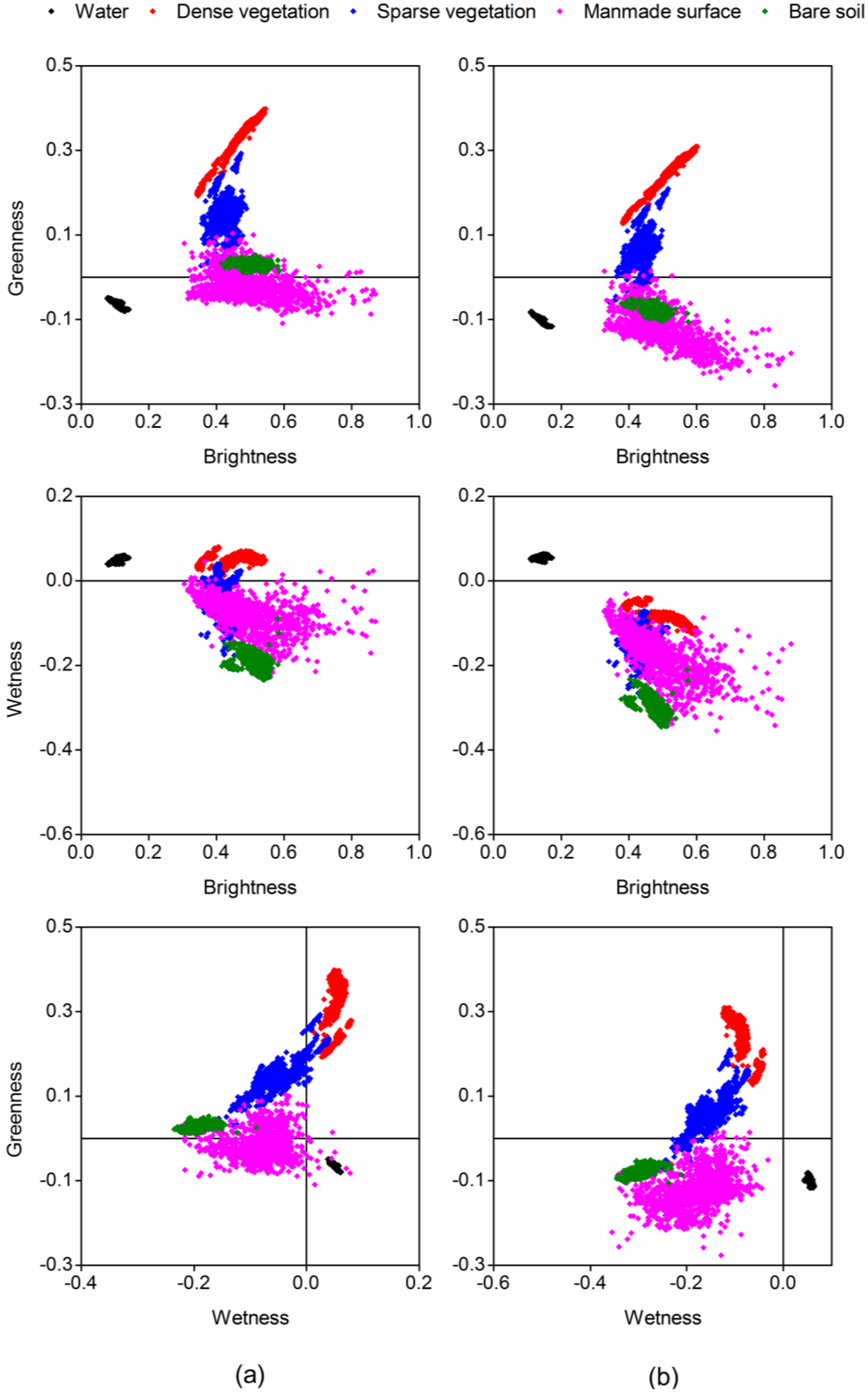
Figure 5). The shapes of the selected samples from the validation scene in the two sets of tasseled cap spaces are similar, whereas their orientation and relative location differ moderately from each other (Figure 5). The greenness and wetness values of our transformation (hereafter referred to as ETM+-based TCT) were generally lower than those of Baig et al. [21] (hereafter referred to as TM-based TCT). In the brightness-greenness space, the greenness values of bare soil samples derived from the TM-based TCT are all greater than 0, and remain stable as the brightness value increases (Figure 5a). On the contrary, the ETM+-based TC transformed space reveals that the greenness values of bare soil samples are all less than 0, and there is a slight decline in its greenness value as the brightness value rises (Figure 5b). Considering that soil has the highest spectral reflectance in the short-wave infrared band (SWIR1, with a central wavelength of 1.609 μm) within the spectral range of Landsat 8 [47], a smaller loading in the SWIR1 band may lead to lower greenness values of bare soil samples obtained after transformation, making it easier to discriminate bare soil pixels from sparse vegetation pixels using the greenness alone (Figure 5). Larger disparities are found in brightness–wetness/wetness–greenness space. Besides deep water, the wetness value of dense vegetation as well as a few sparse vegetation and manmade objects samples derived from TM-based TCT are also greater than 0, which shows it is not possible to distinguish water pixels from dense vegetation pixels effectively by using wetness index only. It is suggested that the ETM+-based TC transformed space could better highlight the discrepancy between water bodies and other land cover types due to the wetness values of all land cover types derived from ETM+-based TCT being negative, except water pixels, and the wetness values increasing as the brightness values generally decrease. Taken together, the vegetation cover could be identified from the land surface using a threshold of Greenness index > 0, while the water body could be easily extracted from a TCTW image using a threshold of TCTW > 0. Therefore, it would be very efficient if the TCT-derived indices were introduced in a classification process.
Figure 5. Comparison of tasseled cap spaces derived by (a) Baig et al. (2014) and (b) this study.
Remotesensing 08 00038 g005

3.3. Validation of Tasseled Cap Transformation

A total of 2667 pseudo-invariant samples, including dense vegetation, deep water and manmade surfaces, were selected randomly as an independent validation dataset. Mean bias error (MBE), mean absolute error (MAE), and root-mean-square error (RMSE) were used to assess the goodness of fit between the OLI-based TC value and the quasi real-time ETM+-based TC value from the two transformations.
MBE = 1 n i = 1 n ( E i O i )
MAE = 1 n i = 1 n | E i O i |
RMSE = 1 n i = 1 n ( E i O i ) 2
where n is the number of provinces, and Ei and Oi are the estimated and observed θv, respectively. The MBE corresponds to the metrics of overestimation (−) and underestimation (+) [48]. The method is perfect when MBE = 0, MAE = 0 and RMSE = 0.
The results achieved in terms of the three TC features are summarized in Table 5. There appeared to be an obvious overestimation of the TM-based TCT greenness (MBE = 0.0588) and wetness values (MBE = 0.0739), though the correlation coefficients of both approaches were significant at the 0.01 level. Although the estimations of brightness from the two methods were comparable, better performance for greenness and wetness was achieved by our method; the R2 increased by 0.0133 and 0.4428, the MAE decreased by 0.0312 and 0.0643, and the RMSE decreased by 0.0414 and 0.0811, respectively. Overall, it can be seen that the transform coefficients of this study can better maintain the tasseled cap features. The estimation accuracy, for the wetness index in particular, improved greatly.
There are several possible explanations for the improvement in our estimation. First, there is continuity between the band settings of Landsat 8 and Landsat 7, as well as some new spectral characteristics including the addition of a deep blue band, a shortwave-infrared band, and refinement of the spectral range of several bands corresponding to those of Landsat 7 ETM+ [49]. These may bring estimation error if the TM TCT coefficients are directly applied to OLI data for creating the target feature space. Second, the DN-based TM TCT coefficients are suitable for raw DN images rather than radiometrically calibrated data. Therefore, an increase in the estimation error is likely when taking the at-satellite OLI images as input data. In addition, many studies have proven the effectiveness of at-satellite reflectance–based TCT coefficients [25,26]; however, the impacts of atmospheric scattering and sun illumination geometry still exist. The direct application of all samples to the images used to calculate the tasseled cap transformation coefficients may also lower the estimation accuracy. Our method has the capability to overcome the deficiencies mentioned above and can thereby obtain relatively accurate tasseled cap transformation indices.
Table 5. Assessment of the two tasseled cap transformations.
TCTIndexR2MBEMAERMSE
Baig et al.Brightness0.97370.01320.03380.0432
Greenness0.98070.05880.05880.0719
Wetness0.54540.07390.07430.0947
This studyBrightness0.98660.04320.04680.0567
Greenness0.9940−0.00930.02760.0305
Wetness0.98810.00100.01000.0136

3.4. Soil Moisture Content Retrieval

The relationship between the TCTW, TVDI and θv could be complicated by the presence of various vegetated conditions in rice paddies during winter [50]. The rice paddy may be partially or fully covered by rice straw, grass, or crop canopy (e.g., rape). This may have a negative effect on the θv retrieval algorithm. It has been reported that the Normalized Difference Tillage Index (NDTI) is a good indicator for differentiating vegetation/crop residue from soil [51,52]. NDTI can be calculated by surface reflectance values from the two shortwave-infrared (SWIR) bands:
NDTI = ρ S W I R 1 ρ S W I R 2 ρ S W I R 1 + ρ S W I R 2
where ρSWIR1 and ρSWIR2 refer to the surface reflectance values from Band 5 and Band 7 in the Landsat-7 ETM+ sensor and Band 6 and Band 7 in the Landsat-8 OLI sensor, respectively. Therefore, as summarized from all the NDTI values at the in situ field samples, the error statistics were calculated for two NDTI classes of <0.2 and ≥0.2. NDTI < 0.2 represented a low fractional crop residue/vegetation cover condition, whereas NDTI ≥ 0.2 indicated a moderate or high fractional crop residue/vegetation cover condition. Moreover, the ground water condition could also be a potential factor of influence for θv estimation. Additionally, it is infeasible to separate the flooded or non-flooded status in paddies from different provinces using a fixed θv threshold, because the saturated volumetric moisture content of paddy soil may differ in terms of variations in soil texture. Thus, we roughly classified the flooded or non-flooded status by visual interpretation. Taken together, during the non-rice growing period (usually from December to February), the rice paddy surface conditions can mainly be classified into four categories: (1) Flooded (NDTI < 0.2); (2) Flooded (NDTI ≥ 0.2); (3) Non-flooded (NDTI < 0.2); and (4) Non-flooded (NDTI ≥ 0.2).
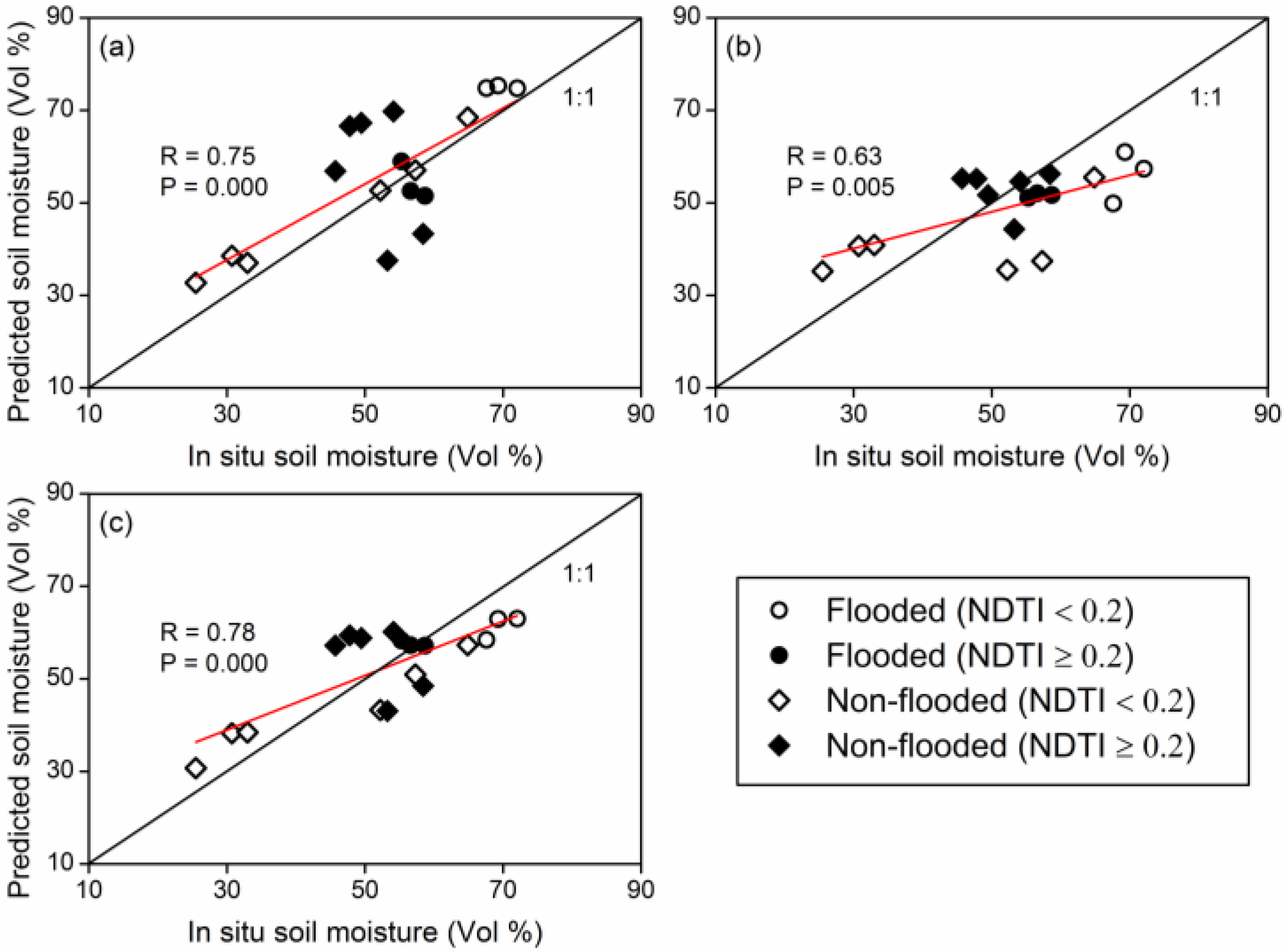
The 64 field samples were randomly separated into training (46/64) and validation (18/64) samples. Different regressor combinations were inputted to the GRNN model in order to investigate the best performance for θv retrieval. Assessing the accuracy was achieved by comparing the estimation results with the in situ measured data in terms of different input configurations (Figure 6). The error statistics (bias, MAE and RMSE) were calculated based on the validation dataset for different scenarios (Table 6). The correlation coefficients of all the input configurations were significant at the 0.01 level. The TCTW+TVDI configuration gave the best performance as an input into the model, with the highest correlation coefficient (R = 0.78, P = 0.000) and lowest estimation errors (MAE = 7.19 and RMSE = 7.83). It seemed to be less effective in estimating θv (for the retrieval process) using either the TCTW or TVDI configuration as the input into the model. The TVDI configuration yielded the largest estimation errors (MAE = 8.94 and RMSE = 10.39), with the lowest correlation coefficient (R = 0.63, P = 0.005). There was an underestimation of 3.69% in the TVDI configuration but an overestimation of 3.54% in the TCTW configuration. More specifically, the TCTW had a problem in estimating the process of θv in non-flooded and vegetated areas, where considerably larger errors (MAE = 15.72, RMSE = 15.90) were produced compared to the samples with respect to other land cover types (Table 6).
Figure 6. Comparison between modeled and in situ measured volumetric surface soil moisture content (θv) with (a) TCTW; (b) TVDI and (c) TCTW+TVDI input configurations.
Remotesensing 08 00038 g006
Table 6. Assessment of the model performance under different scenarios.
Vegetation Coverage ConditionGround Water ConditionMBE (%)MAE (%)RMSE (%)
TCTWNDTI ≥ 0.2Flooded−2.534.965.20
Non-flooded5.4315.7215.90
NDTI < 0.2Flooded5.295.295.63
Non-flooded3.803.894.88
PooledPooled3.548.2510.13
TVDINDTI ≥ 0.2Flooded−5.255.255.39
Non-flooded1.435.146.29
NDTI < 0.2Flooded−13.6013.6014.15
Non-flooded−3.0712.2413.02
PooledPooled−3.698.9410.39
TCTW+TVDINDTI ≥ 0.2Flooded0.701.721.96
Non-flooded3.059.789.96
NDTI < 0.2Flooded−8.208.208.30
Non-flooded−0.786.846.97
PooledPooled−0.497.197.83
The presence of non-paddy rice vegetation, during the non-rice growing period, will increase the greenness signal and reduce the soil signatures as the canopies of green plants or straws partially or fully cover the paddy surface area [53]. It has been suggested that the soil moisture status is the primary characteristic expressed in TCTW, while only a limited amount of plant moisture variation is represented in the tasseled cap space [22]. As a consequence, the TCTW would work well on the condition that the land surface consisted of merely bare soil without any other materials. However, a much higher accuracy was achieved under flooded and vegetated surface conditions than under non-flooded and non-vegetated surface conditions. The cause of this may be that the water signature often dominates over the flooded rice paddy surface, as it is covered by a mixture of rice residue, soil and water bodies, and it then conceals the weakness of TCTW in estimating the soil moisture over vegetated areas. Most of the soil and vegetated surfaces are obscured under flooded conditions.
In contrast to the TCTW configuration, the TVDI configuration failed to estimate θv over the bare soil areas, with the largest range of RMSE (13.02%–14.15%) (Table 6), especially for the samples with a high moisture status (θv > 50%) (Figure 6). Furthermore, there was a high probability of θv underestimation over flooded and bare soil areas (MBE = −13.60%). Mallick et al. [7] pointed out that the estimation results from an LST-VI index method like TVDI or SWI may be less reliable with low fractional vegetation cover because the wet edge is set as a horizontal base of the LST-VI triangle. Despite this, the same situation was observed in our experiment based on the parameters regressed from the sloping wet edge. Hence, we hypothesized that the definition of the wet edge was not a major concern affecting the prediction ability of TVDI. There are several likely causes for the considerably higher estimation error produced by the TVDI method. First, the differences in the optical-thermal infrared spectral bands and the performances of the instruments between Landsat 7 and Landsat 8 can give rise to slight variations in the derived Normalized Difference Vegetation Index (NDVI) and LST data used during the model training and prediction phase. Second, the non-linear stretching effect of NDVI can enhance the low-vegetation cover part within the full fractional vegetation cover range [54], and the NDVI value over the bare soil area may be overestimated to some extent. Third, the land surface emissivity of the bare soil area was simplified to the soil emissivity as a substitution. This may lower the accuracy of the LST retrieval over the bare soil area. Because of this, the model parameters were not perfectly regressed, the prediction ability of TVDI decreased over the bare area. It can therefore be assumed that the combination of TCTW and TVDI can provide high sensitivity to changes in soil moisture over both sparsely and densely vegetated areas during the fallow period.

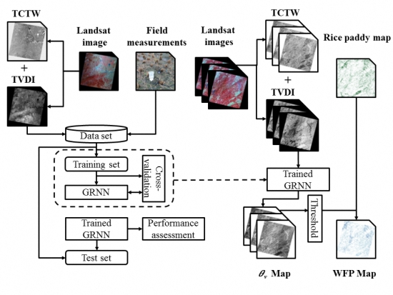
3.5. Extraction of the Winter Continuously Flooded Paddy

After the time series θv images were collected using the TCTW+TVDI configuration modeling, we generated flooded paddy tiles for each 
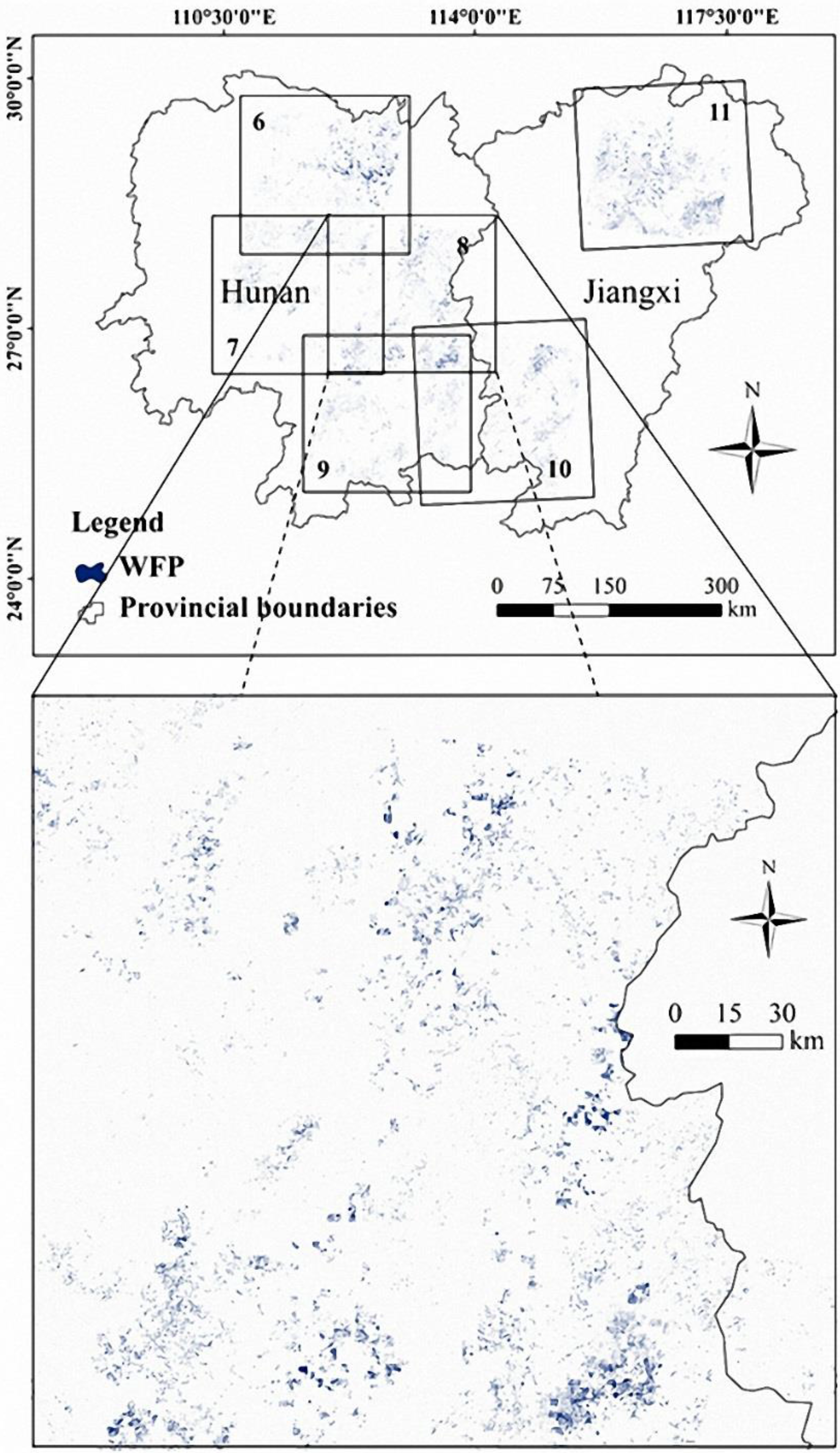
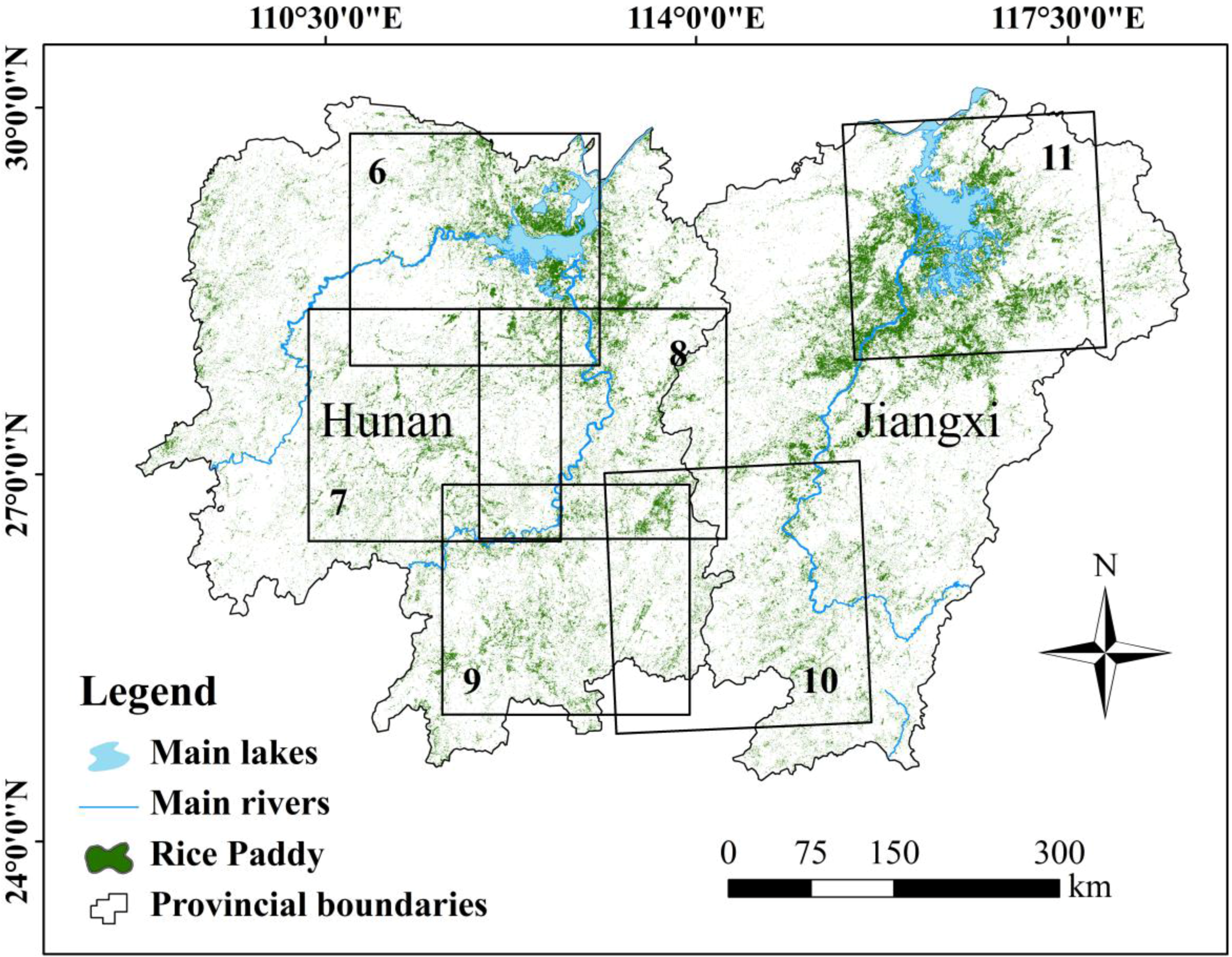
θv image with SMC thresholding over the case study area. Finally, the spatial distribution of WFP represented by the overlapping areas of flooded rice paddies of all three tiles in winter in Hunan and Jiangxi provinces was extracted based on the rice paddy map (Figure 7). Winter flooded paddies were found to be sparsely distributed throughout the main rice planting areas of Hunan and Jiangxi provinces. The amount of WFP around the Dongting Lake and Poyang Lake regions was larger than in the other scenes probably due to the presence of significantly larger amounts of rice paddies. The ratio of the area of WFP to the total area of rice paddy under each Landsat scene coverage was then calculated and summarized in Table 7. The average slope of the map of the case study area was used to classify the scene coverage into flat and hilly areas. The fraction of WFP in flat areas was comparable to that of hilly areas in Hunan, whereas there was an obvious increase in the fraction in flat areas than that of hilly areas in Jiangxi.
Figure 7. Spatial distribution of WFP derived from 2013–2014 Landsat data in selected areas with a zoom of scene #8.
Remotesensing 08 00038 g007
Table 7. Fraction of WFP within Hunan and Jiangxi provinces.
Scene #Path/RowGeographic LocationMean Slope (°)Fraction of WFP (%) *
6124/40Hunan, China3.0914.81
7124/41Hunan, China4.7113.74
8123/41Hunan, China3.2417.56
9123/42Hunan, China5.0015.80
10122/42Jiangxi, China5.3922.15
11121/40Jiangxi, China2.6515.06
* The fraction of WFP represents the ratio of the area of WFP to the total area of rice paddy under the corresponding Landsat scene coverage.
Although Southwest China boasts a well-developed river system and relatively abundant water resources, the complex terrain and large fraction of mountainous areas always result in there being a long distance between the cropland and water sources, increasing the difficulty involved in water resource utilization. Most regions are unable to irrigate during the dry season because they do not possess the necessary water storage facilities, infrastructure and technology. Storing water in winter is an effective method for some areas to ease the pressure on water resource shortages in the rice growing period. However, long-term flooding is one of the main factors causing high CH4 emissions during the rice growing period in southern China. The average CH4 flux from a rice paddy that was flooded in the winter season (about 36.2 g·CH4·m−2) is approximately 1.9 times that from a rice paddy that experienced a drained winter season [3,4,55]. Under these conditions, other rice varieties (e.g., water-saving and drought-resistant rice) and single rice–upland winter crop rotation could be effective options for mitigating CH4 emissions without reducing grain yields under water-saving irrigation in the traditional WFP [55,56]. Therefore, the spatial distribution data of WFP could not only be useful for GHG emissions estimation, but also for guiding the selection of rice varieties and cropping patterns, as well as water resource management in local agricultural production. On the contrary, the plain areas have much better irrigation conditions, and thus there is no need to maintain WFP for supplementing water during the rice growing season.
However, corroboration of a continuous status of flooding remains difficult to fulfill at present. As an alternative solution, confusion matrices were calculated based on the ground-truth dataset to assess the accuracy of flooded paddy identification from the five single-date images in the study area (Table 8). The 18 validation field sites mentioned in Section 3.4, consisting of flooded (6/18) and non-flooded (12/18) samples, were used as the ground-truth dataset, and there was good agreement between the identification result and ground-truth data [57]. Furthermore, we compared our estimate with the result from Yan et al. [58], who suggested 10% as the fractional amount of WFP in the CH4 emissions of both Hunan and Jiangxi. Our results were 15.48% and 18.61%, for the fractional coverage of WFP in the total rice paddy area. This was evident in the case of the comparison between various modeled results and satellite observations, and regional discrepancies were subsequently found (e.g., Sichuan basin) [59]. Moreover, the large dependence on the surface water status data in determining the CH4 emissions has been exemplified in a report by Jonai and Takeuchi [60]. Significant underestimation of the fraction of WFP may result in inconsistencies between modeled results and satellite observations. The validation of the WFP maps derived from remotely sensed data has a long way to go owing to a lack of census statistics. Further efforts should be made to create a validation database consisting of dynamic data collected from regional moisture monitoring networks and surveys from a considerable number of local people.
Table 8. Assessment of the accuracy of flooded paddy identification.
Ground Truth (Pixels)FloodedNon-FloodedTotal
Flooded516
Non-flooded21012
Total71118
Prod. Acc. (%)83.3383.33
User Acc. (%)71.4390.91
Overall accuracy (%)83.33
Kappa coefficient0.64

4. Conclusions

A methodology that combines Landsat-based TCTW and TVDI for regional mapping of flooded paddies over both sparsely and densely vegetated areas has been presented. The implementation and innovative aspects of this methodology are as follows:
First, the new 7-band Landsat 8 OLI TCT coefficients were updated. The result showed that a good separation among different land cover types was apparent after our transformation, with substantially smaller prediction error than the existing transformation coefficients. The improved procedure for TCT derivation can also be extended to other forthcoming multi-spectral remotely sensed data (e.g., Sentinel-2 and Worldview-3), if the target sensor in question has a close similarity with the reference sensor (with known TCT coefficients). Second, this is the first time that a synergistic TCTW/TVDI approach has been performed to estimate surface soil moisture content with Landsat images, and satisfying results with various vegetation cover types and ground water conditions have been achieved. Finally, the WFP was extracted from the overlapping area of the time series imagery of flooded paddies with an accuracy of 83.33%.
The methodology described in this paper can be applied to generate a regional geospatial database of WFP, which can then be used to support various studies of agricultural water use, GHG emissions estimates, and food security in China and Asia. This work can also be considered as an exploratory study for the use of other optical-thermal sensors. To obtain a more accurate WFP map, future efforts may focus on improving the retrieval algorithm in the soil moisture estimation process and using remotely sensed time series imagery with high resolution in both time and space.

Supplementary Files

Supplementary File 1

Acknowledgments

This study was financially supported by the “Strategic Priority Research Program e Climate Change: Carbon Budget and Relevant Issues” of the Chinese Academy of Sciences (No. XDA05020200), the Key Research Program of the Chinese Academy of Sciences (No. KZZD-EW-10-04-2), the Ministry of Science and Technology of China (No. 2012DFG90290) and the Ministry of Agriculture of China (No. 201103039). The authors thank Jiang Yuan from soil and fertilizer research institute, Sichuan Academy of Agricultural Sciences for his assistance in field survey.

Author Contributions

Bolun Li and Xiaoyuan Yan contributed to the experimental design of the study. Bolun Li collected field data, conducted the analysis of results and wrote the manuscript. All authors contributed to writing and reviewing the manuscript.

Conflicts of Interest

The authors declare no conflict of interest.

References

  1. Food and Agriculture Organization of the Unitited Nations (FAO). Available online: http://apps.fao.org/ (accessed on 1 July 2015).
  2. Li, Q. Paddy Soils of China; Science Press: Beijing, China, 1992. (In Chinese) [Google Scholar]
  3. Cai, Z.C.; Tsuruta, H.; Minami, K. Methane emission from rice fields in China: Measurements and influencing factors. J. Geophys. Res. Atmos. 2000, 105, 17231–17242. [Google Scholar] [CrossRef]
  4. Intergovernmental Panel on Climate Change (IPCC). 2006 IPCC Guidelines for National Greenhouse Gas Inventories; Institute for Global Environmental Strategies: Hayama, Japan, 2007. [Google Scholar]
  5. Dubois, P.C.; van Zyl, J.; Engman, T. Measuring soil moisture with imaging radars. IEEE Trans. Geosci. Remote Sens. 1995, 33, 915–926. [Google Scholar] [CrossRef]
  6. Liu, Y.Y.; Dorigo, W.A.; Parinussa, R.M.; de Jeu, R.A.M.; Wagner, W.; McCabe, M.F.; Evans, J.P.; van Dijk, A.I.J.M. Trend-preserving blending of passive and active microwave soil moisture retrievals. Remote Sens. Environ. 2012, 123, 280–297. [Google Scholar] [CrossRef]
  7. Mallick, K.; Bhattacharya, B.K.; Patel, N.K. Estimating volumetric surface moisture content for cropped soils using a soil wetness index based on surface temperature and NDVI. Agric. For. Meteorol. 2009, 149, 1327–1342. [Google Scholar] [CrossRef]
  8. Neusch, T.; Sties, M. Application of the Dubois-model using experimental synthetic aperture Radar data for the determination of soil moisture and surface roughness. ISPRS J. Photogramm. Remote Sens. 1999, 54, 273–278. [Google Scholar] [CrossRef]
  9. Pasolli, L.; Notarnicola, C.; Bertoldi, G.; Della Chiesa, S.; Niedrist, G.; Bruzzone, L.; Tappeiner, U.; Zebisch, M. Soil moisture monitoring in mountain areas by using high-resolution SAR images: Results from a feasibility study. Eur. J. Soil Sci. 2014, 65, 852–864. [Google Scholar] [CrossRef]
  10. Patel, N.R.; Anapashsha, R.; Kumar, S.; Saha, S.K.; Dadhwal, V.K. Assessing potential of MODIS derived temperature/vegetation condition index (TVDI) to infer soil moisture status. Int. J. Remote Sens. 2008, 30, 23–39. [Google Scholar] [CrossRef]
  11. Prakash, R.; Singh, D.; Pathak, N.P. A fusion approach to retrieve soil moisture with SAR and optical data. IEEE J. Sel. Top. Appl. Earth Obs. Remote Sens. 2012, 5, 196–206. [Google Scholar] [CrossRef]
  12. Sandholt, I.; Rasmussen, K.; Andersen, J. A simple interpretation of the surface temperature/vegetation index space for assessment of surface moisture status. Remote Sens. Environ. 2002, 79, 213–224. [Google Scholar] [CrossRef]
  13. Wang, C.; Qi, J.; Moran, S.; Marsett, R. Soil moisture estimation in a semiarid rangeland using ERS-2 and TM imagery. Remote Sens. Environ. 2004, 90, 178–189. [Google Scholar] [CrossRef]
  14. Moran, M.S.; Clarke, T.R.; Inoue, Y.; Vidal, A. Estimating crop water deficit using the relation between surface-air temperature and spectral vegetation index. Remote Sens. Environ. 1994, 49, 246–263. [Google Scholar] [CrossRef]
  15. Barrett, B.; Dwyer, E.; Whelan, P. Soil moisture retrieval from active spaceborne microwave observations: An evaluation of current techniques. Remote Sens. 2009, 1, 210–242. [Google Scholar] [CrossRef]
  16. Carlson, T. An overview of the “triangle method” for estimating surface evapotranspiration and soil moisture from satellite imagery. Sensors 2007, 7, 1612–1629. [Google Scholar] [CrossRef]
  17. Carlson, T.N.; Gillies, R.R.; Perry, E.M. A method to make use of thermal infrared temperature and NDVI measurements to infer surface soil water content and fractional vegetation cover. Remote Sens. Rev. 1994, 9, 161–173. [Google Scholar] [CrossRef]
  18. Shafian, S.; Maas, S. Index of soil moisture using raw Landsat image digital count data in texas high plains. Remote Sens. 2015, 7, 2352–2372. [Google Scholar] [CrossRef]
  19. Zhang, D.; Tang, R.; Zhao, W.; Tang, B.; Wu, H.; Shao, K.; Li, Z.-L. Surface soil water content estimation from thermal remote sensing based on the temporal variation of land surface temperature. Remote Sens. 2014, 6, 3170–3187. [Google Scholar] [CrossRef] [Green Version]
  20. Wang, C.; Qi, S.; Niu, Z.; Wang, J. Evaluating soil moisture status in China using the temperature–vegetation dryness index (TVDI). Can. J. Remote Sens. 2004, 30, 671–679. [Google Scholar] [CrossRef]
  21. Baig, M.H.A.; Zhang, L.; Shuai, T.; Tong, Q. Derivation of a tasselled cap transformation based on Landsat 8 at-satellite reflectance. Remote Sens. Lett. 2014, 5, 423–431. [Google Scholar] [CrossRef]
  22. Crist, E.P.; Cicone, R.C. A physically-based transformation of thematic mapper data—The TM tasseled cap. IEEE Trans. Geosci. Remote Sens. 1984, GE-22, 256–263. [Google Scholar] [CrossRef]
  23. Crist, E.P.; Cicone, R.C. Application of the tasseled cap concept to simulated thematic mapper data. Photogramm. Eng. Remote Sens. 1984, 50, 343–352. [Google Scholar]
  24. Horne, J.H. A tasseled cap transformation for Ikonos images. In Proceedings of the ASPRS 2003 Annual Conference Proceedings, Anchorage, AK, USA, 3–9 May 2003; pp. 1–7.
  25. Huang, C.; Wylie, B.; Yang, L.; Homer, C.; Zylstra, G. Derivation of a tasselled cap transformation based on Landsat 7 at-satellite reflectance. Int. J. Remote Sens. 2002, 23, 1741–1748. [Google Scholar] [CrossRef]
  26. Ivits, E.; Lamb, A.; Langar, F.; Hemphill, S.; Koch, B. Orthogonal transformation of segmented SPOT5 images. Photogramm. Eng. Remote Sens. 2008, 74, 1351–1364. [Google Scholar] [CrossRef]
  27. Kauth, R.J.; Thomas, G. The tasselled cap-a graphic description of the spectral-temporal development of agricultural crops as seen by Landsat. In Proceedings of the Symposium on Machine Processing of Remotely Sensed Data, Purdue University, West Lafayette, IN, USA, 29 June–1 July 1976; pp. 4B41–4B51.
  28. Lobser, S.E.; Cohen, W.B. MODIS tasselled cap: Land cover characteristics expressed through transformed MODIS data. Int. J. Remote Sens. 2007, 28, 5079–5101. [Google Scholar] [CrossRef]
  29. Hoan, N.T.; Tateishi, R.; Dong Xuan, P.; Johnson, B. Global water mapping using MODIS tasseled cap indexes. In Proceedings of the 2012 IEEE International Geoscience and Remote Sensing Symposium (IGARSS), Munich, Germany, 22–27 July 2012; pp. 7161–7164.
  30. Delta-T Devices. Available online: http://www.delta-t.co.uk/ (accessed on 13 September 2015).
  31. Delta-T Devices. Product Support Material. Available online: http://www.delta-t.co.uk/product-support-material.asp/ (accessed on 13 September 2015).
  32. U.S. Geological Survey (USGS). Frequently Asked Questions about the Landsat Missions. Available online: http://landsat.usgs.gov/band_designations_landsat_satellites.php/ (accessed on 22 March 2015).
  33. Geospatial Data Cloud. Available online: http://www.gscloud.cn/ (accessed on 5 April 2014).
  34. U.S. Geological Survey (USGS). Using the USGS Landsat 8 product. Available online: http://landsat.usgs.gov/landsat8_using_product.php/ (accessed on 22 March 2015).
  35. Zhu, Z.; Wang, S.; Woodcock, C.E. Improvement and expansion of the Fmask algorithm: Cloud, cloud shadow, and snow detection for Landsats 4–7, 8, and Sentinel 2 images. Remote Sens. Environ. 2015, 159, 269–277. [Google Scholar] [CrossRef]
  36. Li, B.; Ti, C.; Yan, X. Estimating rice paddy areas in China using multi-temporal NDVI imagery based on change detection. Pedosphere. accepted.
  37. Institute of Soil Science, Chinese Academy of Sciences (ISSAS). Soil information system of china (SISChina). Available online: http://www.issas.cas.cn/ztwz/200910/t20091015_2551708.html/ (accessed on 15 May 2015).
  38. Schløler, H.; Hartmann, U. Mapping neural network derived from the parzen window estimator. Neural Netw. 1992, 5, 903–909. [Google Scholar] [CrossRef]
  39. Specht, D.F. A general regression neural network. IEEE Trans. Neural Netw. 1991, 2, 568–576. [Google Scholar] [CrossRef] [PubMed]
  40. Bauer, M.M. General Regression Neural Network, Grnn: A Neural Network for Technical Use; University of Wisconsin: Madison, WI, USA, 1995. [Google Scholar]
  41. Jia, K.; Liang, S.; Liu, S.; Li, Y.; Xiao, Z.; Yao, Y.; Jiang, B.; Zhao, X.; Wang, X.; Xu, S.; et al. Global land surface fractional vegetation cover estimation using general regression neural networks from MODIS surface reflectance. IEEE Trans. Geosci. Remote Sens. 2015, 53, 4787–4796. [Google Scholar] [CrossRef]
  42. Baker, B.D. Can flexible non-linear modeling tell us anything new about educational productivity? Econ. Educ. Rev. 2001, 20, 81–92. [Google Scholar] [CrossRef]
  43. Cigizoglu, H.K. Generalized regression neural network in monthly flow forecasting. Civ. Eng. Environ. Syst. 2005, 22, 71–81. [Google Scholar] [CrossRef]
  44. Ibrić, S.; Jovanović, M.; Djurić, Z.; Parojčić, J.; Solomun, L. The application of generalized regression neural network in the modeling and optimization of aspirin extended release tablets with EUDRAGIT® RS PO as matrix substance. J. Controll. Release 2002, 82, 213–222. [Google Scholar] [CrossRef]
  45. Leung, M.T.; Chen, A.-S.; Daouk, H. Forecasting exchange rates using general regression neural networks. Comput. Oper. Res. 2000, 27, 1093–1110. [Google Scholar] [CrossRef]
  46. Panda, B.; Bahubalendruni, M.V.A.R.; Biswal, B. A general regression neural network approach for the evaluation of compressive strength of FDM prototypes. Neural Comput. Appl. 2015, 26, 1129–1136. [Google Scholar] [CrossRef]
  47. Richards, J.A. Remote Sensing Digital Image Analysis; Springer: Heidelberg, Germany, 1999. [Google Scholar]
  48. Holzman, M.E.; Rivas, R.; Piccolo, M.C. Estimating soil moisture and the relationship with crop yield using surface temperature and vegetation index. Int. J. Appl. Earth Obs. Geoinform. 2014, 28, 181–192. [Google Scholar] [CrossRef]
  49. Li, P.; Jiang, L.; Feng, Z. Cross-comparison of vegetation indices derived from Landsat-7 Enhanced Thematic Mapper Plus (ETM+) and Landsat-8 Operational Land Imager (OLI) sensors. Remote Sens. 2013, 6, 310–329. [Google Scholar] [CrossRef]
  50. Xing, G.; Zhao, X.; Xiong, Z.; Yan, X.; Xu, H.; Xie, Y.; Shi, S. Nitrous oxide emission from paddy fields in China. Acta Ecol. Sin. 2009, 29, 45–50. [Google Scholar] [CrossRef]
  51. Zhang, R.; Tian, J.; Su, H.; Sun, X.; Chen, S.; Xia, J. Two improvements of an operational two-layer model for terrestrial surface heat flux retrieval. Sensors 2008, 8, 6165–6187. [Google Scholar] [CrossRef]
  52. Van Deventer, A.; Ward, A.; Gowda, P.; Lyon, J. Using thematic mapper data to identify contrasting soil plains and tillage practices. Photogramm. Eng. Remote Sens. 1997, 63, 87–93. [Google Scholar]
  53. Huete, A.R.; Jackson, R.D.; Post, D.F. Spectral response of a plant canopy with different soil backgrounds. Remote Sens. Environ. 1985, 17, 37–53. [Google Scholar] [CrossRef]
  54. Purevdorj, T.S.; Tateishi, R.; Ishiyama, T.; Honda, Y. Relationships between percent vegetation cover and vegetation indices. Int. J. Remote Sens. 1998, 19, 3519–3535. [Google Scholar]
  55. Yan, X.; Yagi, K.; Akiyama, H.; Akimoto, H. Statistical analysis of the major variables controlling methane emission from rice fields. Glob. Chang. Biol. 2005, 11, 1131–1141. [Google Scholar] [CrossRef]
  56. Xu, Y.; Ge, J.; Tian, S.; Li, S.; Nguy-Robertson, A.L.; Zhan, M.; Cao, C. Effects of water-saving irrigation practices and drought resistant rice variety on greenhouse gas emissions from a no-till paddy in the central lowlands of China. Sci. Total Environ. 2015, 505, 1043–1052. [Google Scholar] [CrossRef] [PubMed]
  57. Landis, J.R.; Koch, G.G. The measurement of observer agreement for categorical data. Biometrics 1977, 33, 159–174. [Google Scholar] [CrossRef] [PubMed]
  58. Yan, X.; Akiyama, H.; Yagi, K.; Akimoto, H. Global estimations of the inventory and mitigation potential of methane emissions from rice cultivation conducted using the 2006 intergovernmental panel on climate change guidelines. Glob. Biogeochem. Cycles 2009, 23, GB2002. [Google Scholar] [CrossRef]
  59. Hayashida, S.; Ono, A.; Yoshizaki, S.; Frankenberg, C.; Takeuchi, W.; Yan, X. Methane concentrations over monsoon asia as observed by sciamachy: Signals of methane emission from rice cultivation. Remote Sens. Environ. 2013, 139, 246–256. [Google Scholar] [CrossRef]
  60. Jonai, H.; Takeuchi, W. Comparison between global rice paddy field mapping and methane flux data from gosat. In Proceedings of the 2014 IEEE International Geoscience and Remote Sensing Symposium (IGARSS), Quebec, QC, Canada, 13–18 July 2014; pp. 2098–2101.

