Mapping Forest Canopy Height Across Large Areas by Upscaling ALS Estimates with Freely Available Satellite Data

Abstract

Operational assessment of forest structure is an on-going challenge for land managers, particularly over large, remote or inaccessible areas. Here, we present an easily adopted method for generating a continuous map of canopy height at a 30 m resolution, demonstrated over 2.9 million hectares of highly heterogeneous forest (canopy height 0–70 m) in Victoria, Australia. A two-stage approach was utilized where Airborne Laser Scanning (ALS) derived canopy height, captured over ~18% of the study area, was used to train a regression tree ensemble method; random forest. Predictor variables, which have a global coverage and are freely available, included Landsat Thematic Mapper (Tasselled Cap transformed), Moderate Resolution Imaging Spectroradiometer Normalized Difference Vegetation Index time series, Shuttle Radar Topography Mission elevation data and other ancillary datasets. Reflectance variables were further processed to extract additional spatial and temporal contextual and textural variables. Modeled canopy height was validated following two approaches; (i) random sample cross validation, and (ii) with 108 inventory plots from outside the ALS capture extent. Both the cross validation and comparison with inventory data indicate canopy height can be estimated with a Root Mean Square Error (RMSE) of ≤ 31% (~5.6 m) at the 95th percentile confidence interval. Subtraction of the systematic component of model error, estimated from training data error residuals, rescaled canopy height values to more accurately represent the response variable distribution tails e.g., tall and short forest. Two further experiments were carried out to test the applicability and scalability of the presented method. Results suggest that (a) no improvement in canopy height estimation is achieved when models were constructed and validated for smaller geographic areas, suggesting there is no upper limit to model scalability; and (b) training data can be captured over a small percentage of the study area (~6%) if response and predictor variable variance is captured within the training cohort, however RMSE is higher than when compared to a stratified random sample.

1. Introduction

For large, inaccessible and remote forested areas, the assessment of vegetation structure in an operational framework remains an on-going challenge for land managers [1,2,3]. Synoptic capture of large forested areas is provided by space borne passive optical remote sensing platforms and has proved useful for the attribution of forest structure [1,4,5,6,7]. However, the inability of passive instruments to sense below the principal canopy limits their applicability for assessing three-dimensional forest structure attributes, such as canopy height [8,9,10]. Over the last two decades, Light Detection and Ranging (LiDAR) technologies, and in particular discrete return Airborne Laser Scanners (ALS), have become an operational alternative to traditional forest inventory [2,11,12]. Consequently, there has been recent interest in the fusion of ALS and satellite multispectral imagery for the improved retrieval of vegetation parameters (see review by Torabzadeh et al. [13]). However, although examples of acquisition of ALS over very large areas exist [2,14,15,16,17,18], ALS coverage is often incomplete and follows a transect or linear pattern and is therefore inappropriate for deriving wall-to-wall maps of vegetation structure.

To achieve large area attribution, ALS can be used as a sampling tool in a two-stage approach where ALS is captured over a fraction of the study area. This is achieved by first establishing an empirical statistical model between ALS metrics and spectral reflectance and/or other spatially synoptic datasets. The model is then applied to the reflectance/synoptic data and therefore upscales estimates of canopy structure beyond the confines of the ALS survey extent [19,20,21,22,23,24]. Examples where assessment has been carried out over large areas of heterogeneous forest include Asner et al. [15] who estimated forest biomass across ~4 million hectares of Peruvian rainforest and Wulder and Seemann [25] who estimated canopy height over 700,000 ha of boreal forest in Canada. Both studies used a linear regression of ALS derived variables with segmented Landsat imagery to predict canopy structure. Continental and global maps of forest structure have also been produced using this method where LiDAR data from the spaceborne the Geoscience Laser Altimeter System (GLAS) sensor was used as a sampling tool in conjunction with coarse resolution satellite imagery (250–1000 m) [26,27,28].

Modeling approaches that have determined a parametric association between response and predictor variables have been successfully applied to the attribution of forest structure [20,22,25]. However, in more recent years machine learning techniques have been utilized for remote sensing applications, where the complex statistical associations of multi-source datasets require more advanced approaches to characterize forests over large areas [19,23,29]. A machine learning technique that has gained in popularity is random forest, an ensemble regression tree technique from the Classification and Regression Tree or CART family [30]. Random forest works by constructing “weak” regression trees (usually in the order of hundreds) from bootstrapped samples of input variables. The “weak” regression trees are then aggregated in an ensemble to produce a robust model that is insensitive to collinear predictor variables and a non-normal distributed response variable [31]. Furthermore, the ease of application (e.g., only two model parameters, see Section 2.3.1) and the ability to run efficiently over large datasets makes random forest an ideal choice for large area attribution [32]. A number of studies have utilized random forest for mapping forest attributes with remotely sensed data, including biomass [28,33], species extent [34], forest extent [21,35,36], canopy cover [7,37,38] and canopy height [24,26,38,39,40,41].

The majority of studies use a combination of predictor variables that can be roughly split into two cohorts: (a) variables that respond to changes in vegetation and are derived from surface reflectance, and (b) variables that determine vegetation growth potential (in the absence of disturbance) such as site quality and climate. Particular choices of predictor datasets are dictated by the target variable, scale of analysis and data costs or accessibility; the ready access to free satellite imagery has been recognized as crucial for the long term modeling of environmental systems [42]. Large area forest assessment should be consistent across the domain of the study, providing an accurate estimate of forest structure regardless of forest type, as well as being locally relevant, for example identifying features in the landscape [6]. An earth observing platform that has proved useful in this respect is the Landsat program, for example, 9 of the 11 random forest studies listed above used Landsat products as a predictor variable in some way.

Random Forest is capable of efficiently incorporating a large number of both continuous and categorical variables, as a result of sub-sampling predictor variables at each node when constructing regression trees. From a remote sensing perspective, this enables additional contextual or textural variables (and the large number of variables this can produce) to be easily incorporated into modeling [43]. The addition of first and second order textural information from satellite imagery has been shown to improve the classification accuracy of forest structure [43,44,45,46]. Additionally, the incorporation of variables generated from a remote sensing time series have also improved model performance. For example, when estimating canopy height Ahmed et al. [38] included a time-since-disturbance variable generated from a Landsat ETM time series, which led to improvements in RMSE of ~20%.

This manuscript extends the work of previous authors by presenting a method for the production of a medium-resolution (30 m) continuous map of canopy height, for a large area (millions of hectares) of highly heterogeneous forest, using freely available datasets as predictive variables and in an open source computing framework. The presented method is intended to be easily adopted (and adapted) by forest scientists and land management agencies for the routine assessment of canopy height. Canopy height was chosen as a candidate metric owing to its importance across many applications including biomass estimation [15,47,48], habitat assessment [49,50] and forest inventory [51,52,53]. An estimate of canopy height is also required to fulfill international assessment and reporting obligations such as those outlined in the Montreal process [54].

2. Materials and Methods

2.1. Study Area

The study area is located in the state of Victoria, Australia (Figure 1A) and comprises a total area of 4 million ha, an area similar in size to the country of Switzerland or the US state of Maryland. Land tenure is predominantly public (> 70%), the majority of which is located in state forest and national parks; the remainder is privately owned and primarily used for grazing livestock. Within this boundary, forest covers 2.9 million ha [35] where forest is defined as “having the potential to reach > 2 m in height and > 20% canopy cover” [55] (Figure 1D). Canopy height across the study area ranges from 0–70 m (Figure 1B).

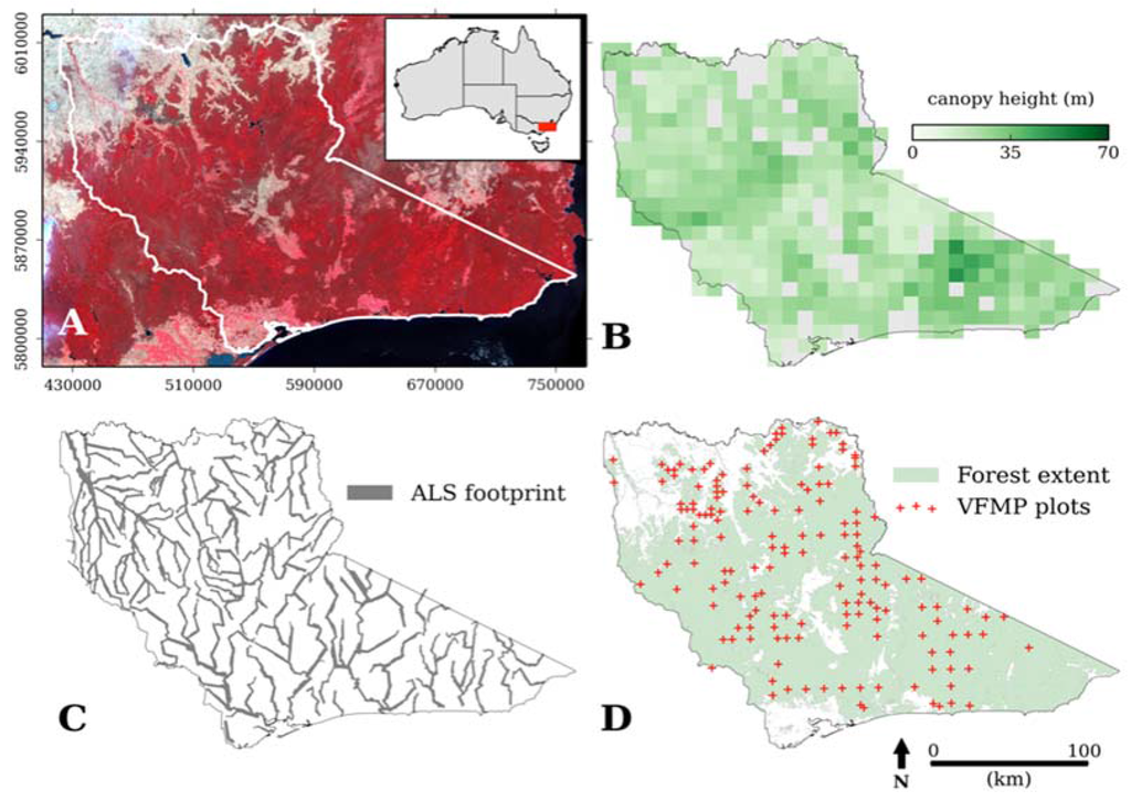
Figure 1. Study area in east Victoria, Australia. A mosaic of 5 Landsat TM false color composite images covering the study area (outlined in white) and location of the study area within Australia (inset) (A). Canopy height derived from ALS capture where canopy height values are aggregated into 10 × 10 km cells (grey indicates no data) (B). The extent of the ALS capture (C). Forest extent [35] and location of Victorian Forest Monitoring Programme forest inventory plots (VFMP) (D). Map coordinate system is the projected Map Grid of Australia (MGA) zone 55.

Figure 1. Study area in east Victoria, Australia. A mosaic of 5 Landsat TM false color composite images covering the study area (outlined in white) and location of the study area within Australia (inset) (A). Canopy height derived from ALS capture where canopy height values are aggregated into 10 × 10 km cells (grey indicates no data) (B). The extent of the ALS capture (C). Forest extent [35] and location of Victorian Forest Monitoring Programme forest inventory plots (VFMP) (D). Map coordinate system is the projected Map Grid of Australia (MGA) zone 55.

The forested area extends across seven seven Interim Biogeographic Regionalisation for Australia (IBRA) regions, IBRA regions have distinct ecological, geological and climatological features [56]. Vegetation is dominated by dry sclerophyll forest and woodlands, which have a relatively sparse canopy and a patchy, scrubby understorey. In the foothills of the Australian Alps there are areas of highly-productive wet forest and rainforest characterized by a tall (> 40 m) and closed canopy with high species richness [57]. There are also subalpine and alpine areas in the Australian Alps that straddle the middle of the study area; these are characterized by relatively short vegetation.

Two factors confound the estimation of canopy height in the study area when using remote sensing. Firstly, the area is subject to regular disturbance from fuel reduction burns, bush fires and drought. For example, the area experienced the most severe drought in a century in the decade prior to the study, which led to large-scale tree mortality [58,59]. Secondly, the physiology of Eucalypt trees and stands, such as an erectophile leaf angle distribution, asymmetrical crown configuration, low foliage density and leaf and crown clumping [60] increase the proportion of reflectance coming from the ground, mid and understorey as well as increasing the shadow fraction [7,61].

2.2. Data Collection

2.2.1. Forest Inventory

Forest inventory plot data was collected as part of the Department of Environment, Land, Water and Planning (DELWP) Victorian Forest Monitoring Programme (VFMP). A total of 130 forest inventory plots were within the study area including 22 that intersected the ALS acquisition extent. Forest inventory plots were installed between May 2011 and December 2014, where at each sampling location a 0.04 ha plot was established following DELWP protocol [62]. Measurements for all trees within the forest inventory plot included diameter at breast height, species and live status. For a subset of trees (including the three tallest) height was also recorded. Dominant canopy height, the mean height of the three tallest live trees in a forest inventory plot, was calculated as the metric summarizing canopy height [63].

2.2.2. Airborne Laser Scanning Data

Airborne Laser Scanning (ALS) data was acquired as part of the DELWP River Health Programme [14]. ALS instrument and survey specifications are presented in Table 1. The ALS data was originally acquired to assess stream bank condition and therefore capture was restricted to the riparian zone, extending 300 m on either side of the river or stream. Flight lines followed the course of the rivers and streams and were therefore off cardinal (Figure 1C), this resulted in a substantial and multiple overlap at flight line intersections. A combination of pulse density and the ability of the two ALS instruments utilized to record up to 4 discrete returns per outgoing laser pulse meant the data was suitable for characterizing vegetation structure [1,64].

The ALS acquisition extent was clipped to the existing forest area [29] and totaled 520,000 ha (Figure 1C). A regular grid with a 250 m spacing (to reduce the spatial autocorrelation of the response variable) was placed over the study area and a total of 12,000 ALS plots were extracted using random stratified sampling. To capture canopy structural variance across the study area, the IBRA bioregion layer was used to stratify the area into distinctive vegetation types. ALS plots that either intersected the edge of the ALS acquisition or had a pulse density < 0.5 pulses·m⁻² [64] were removed from analysis. This resulted in ~11,000 ALS plots for model construction and evaluation.

Table 1. ALS capture and instrument specifications.

Specifications
Capture specifications
Date	December 2009–January 2011
Flying height	600–1500 m above ground level
Mean pulse density	9.4 pl m−2
Swath overlap	20%
Absolute vertical accuracy	± 20 cm
Absolute horizontal accuracy	± 30 cm
Mean footprint diameter	~35 cm
Instrument specifications
Instrument	Leica ALS50-II and ALS60 (Heerbrugg, Switzerland)
Operating wavelength	1064 nm
Max off-nadir scan angle	± 15°
Outgoing pulse rate	36.4 Hz

Table 1. ALS capture and instrument specifications.

Specifications
Capture specifications
Date	December 2009–January 2011
Flying height	600–1500 m above ground level
Mean pulse density	9.4 pl m−2
Swath overlap	20%
Absolute vertical accuracy	± 20 cm
Absolute horizontal accuracy	± 30 cm
Mean footprint diameter	~35 cm
Instrument specifications
Instrument	Leica ALS50-II and ALS60 (Heerbrugg, Switzerland)
Operating wavelength	1064 nm
Max off-nadir scan angle	± 15°
Outgoing pulse rate	36.4 Hz

Square plots (50 m × 50 m) were extracted from the ALS dataset, after computation of canopy height plots were clipped to 30 m × 30 m to be consistent with Landsat TM pixel dimensions. Plots were initially extracted at larger plot dimensions to ensure points around the plot edge had a large enough neighborhood to create a representative ground surface model. Point height data was normalized to ground surface by first classifying points into either ground or non-ground, then using ground classified returns only, creating a triangulated irregular network (TIN) surface. Using the TIN, the ground normalized height for all points was then calculated. Point classification, TIN creation and height normalization were computed using LAStools (version 130225) [65]. The 95th percentile of return height for returns classified as non-ground was calculated for each plot as an analogue of dominant canopy height.

2.2.3. Satellite Imagery and Ancillary Data

A full list of predictor variables initially processed is presented in Table 2. A total of 10 Landsat Thematic Mapper (TM) images were acquired for two seasons; January–March 2009 (summer) and October–November 2009 (spring). Two seasons were acquired as different vegetation cover and composition characteristics are evident at different times of year. For example, imagery captured in summer maximizes the spectral difference between evergreen (overstorey) and cured grass whereas spring imagery captures the green flush [29]. Images were geo-rectified and corrected for atmospheric and bi-directional reflectance distribution function effects to obtain surface reflectance [66], before being mosaicked. Both image mosaics were captured at a time (pre- and post- summer equinox) when sun angle was relatively high to minimize shadow. Although the summer imagery was captured approximately one year prior to the start of the ALS acquisition, imagery from summer 2010 was significantly cloud affected and therefore unsuitable.

A Tasselled Cap (TC) transformation [67] was applied to the Landsat TM mosaics, reducing the 6 visible bands to 3 features: brightness, greenness and wetness [38,39,43]. From each TC feature, 2 first order texture metrics (mean and variance or contextual and textural metrics, respectively) were calculated using a range of kernel sizes (3, 5, 15, 33, 65 and 99 Landsat TM pixels). Maximum kernel size was determined using semivariance analysis of ALS derived canopy height models (30 m × 30 m resolution) captured over three representative forest areas in Victoria [68]. Smaller kernel sizes were used to capture forest structure variance for forests that have a shorter lag and also to characterize forest patches smaller than a continuous canopy e.g., fragmented forests or linear features such as riparian vegetation.

Table 2. List of predictor variables with original image resolution in brackets (⁺kernel sizes: 3, 5, 15, 31, 65, and 99 pixels).

Source
Landsat TM (30 m)	MOD13Q1 (NDVI) time series (2001–2010) (250 m)
Tasselled Cap features and	Summer mean
NDVI	Summer standard deviation
Summer brightness	Summer coefficient of variation
Summer greenness	Summer linear regression slope coefficient
Summer wetness	Spring mean
Spring brightness	Spring standard deviation
Spring greenness	Spring coefficient of variation
Spring wetness	Spring linear regression slope coefficient
Summer NDVI	SRTM (~30 m)
Spring NDVI	Elevation
	Aspect
Image context/texture+	Slope
Summer mean brightness	Climatic (1 km) [66]
Summer mean greenness	Total annual precipitation
Summer mean wetness	Mean annual temperature
Spring mean brightness	Soils
Spring mean greenness	Soil moisture (1 km) [67]
Spring mean wetness	Major soil type (vector) [68]
Summer brightness variance	Coordinates (MGA zone 55) (30 m)
Summer greenness variance	X location
Summer wetness variance	Y location
Spring brightness variance
Spring greenness variance
Spring wetness variance

Table 2. List of predictor variables with original image resolution in brackets (⁺kernel sizes: 3, 5, 15, 31, 65, and 99 pixels).

Source
Landsat TM (30 m)	MOD13Q1 (NDVI) time series (2001–2010) (250 m)
Tasselled Cap features and	Summer mean
NDVI	Summer standard deviation
Summer brightness	Summer coefficient of variation
Summer greenness	Summer linear regression slope coefficient
Summer wetness	Spring mean
Spring brightness	Spring standard deviation
Spring greenness	Spring coefficient of variation
Spring wetness	Spring linear regression slope coefficient
Summer NDVI	SRTM (~30 m)
Spring NDVI	Elevation
	Aspect
Image context/texture+	Slope
Summer mean brightness	Climatic (1 km) [66]
Summer mean greenness	Total annual precipitation
Summer mean wetness	Mean annual temperature
Spring mean brightness	Soils
Spring mean greenness	Soil moisture (1 km) [67]
Spring mean wetness	Major soil type (vector) [68]
Summer brightness variance	Coordinates (MGA zone 55) (30 m)
Summer greenness variance	X location
Summer wetness variance	Y location
Spring brightness variance
Spring greenness variance
Spring wetness variance

A time series of the Moderate Resolution Imaging Spectroradiometer (MODIS) Normalized Difference Vegetation Index (NDVI) product (MOD13Q1) was utilized to capture changes in vegetation structure in the decade prior to the study period. The MODIS NDVI product was chosen as it is highly correlated with vegetation phenology [69] and also has the highest spatial resolution of MODIS products (250 m). Two scenes (summer and spring) were acquired for each year between 2000–2010, where images were captured at the same time each year (first week of February and first week of November, respectively). Images were subsequently ordered into a chronological stack (for each season) and four statistics were computed for each pixel stack: mean, standard deviation, coefficient of variation and the slope coefficient of a linear regression of NDVI with acquisition year.

Site quality and climatological variables can constrain maximum canopy height, for example, a forest plots topographical position or air temperature [61,70]. To capture this within the predictive model, additional variables included elevation, slope and aspect derived from the Shuttle Radar Topography Mission (SRTM) 1 arc-second resolution (~30 m) dataset; mean annual temperature and mean total rainfall [71]; soil water balance [72] and major soil type [73]. Additionally Cartesian coordinate layers (X and Y location) were included [33]. All datasets were resampled to a 30 m resolution to match that of Landsat TM and reprojected to MGA zone 55.

2.3. Canopy Height Estimation with Random Forest

For the estimation of canopy height, random forest was run in ‘regression’ mode where canopy height was the response (dependent) variable and the satellite and ancillary data were the predictor (independent) variables. In order to preserve the spatial heterogeneity present in native forests managed for conservation [61,74,75], canopy height output is computed as a continuous surface i.e. not segmented into forest stands. Random forest models were constructed and validated over the entire study area by randomly sampling 5000 ALS plots from the global dataset in a bootstrap (N = 50). For each bootstrap iteration, the resulting random forest model was applied to a withheld random sample of 1000 ALS plots, from which Root Mean Squared Error (RMSE) was estimated. Outliers at the 95th percentile confidence interval were removed from RMSE calculations. To produce a wall-to-wall map of canopy height, individual random forest models from the bootstrapped cross-validation were combined, to improve generalization, and then applied to the synoptic datasets. A second validation was achieved by comparing forest inventory measured canopy height from outside ALS acquisition area with model output.

Two further experiments were conducted to assess the suitability and applicability of random forest for estimating canopy height over large areas: (a) models were constructed and validated using ALS data within smaller geographic extents, and (b) models were constructed from smaller geographic subsets and validated using ALS data from the remaining portion of the study area. For experiment (a), the hypothesis was that improvements can be made in performance by constructing and validating models over smaller geographic areas owing to the reduced range and variability of the response and predictor variables. Experiment (a) was evaluated by dividing the study area into 24 grid squares (50 km × 50 km), then for each grid square a model was constructed using 75% of ALS plots as training data and the remainder for validation.

LiDAR surveys usually cover a much smaller extent than the River Health capture. Experiment (b) therefore tested the possibility of combining disparate acquisitions to estimate canopy height over a larger area. This was achieved by randomly sampling the twenty-four 50 km × 50 km grid squares, where the number of squares included was iteratively increased from 2 to 23 (5%–95% of the ALS footprint or 1%–16% of the forested area). ALS plot data from the selected grids was combined and used as a training sample, creating a non-random distribution of training samples. A random sample of 2000 ALS plots from outside the selected grid squares were used as validation. An additional 18,000 ALS plots were randomly extracted from the River Health dataset (using the method described in Section 2.2.2), and combined with 2000 from the original sample to create a randomly distributed dataset for the entire study area (i.e., not stratified by IBRA bioregion).

2.3.1. Random Forest Implementation

To facilitate the uptake of this method by land management agencies and forest scientists, computation was achieved using an open source framework [29]. ForestLAS [76] and LAStools [65] were used to extract and process ALS data; GRASS [77] and QGIS [78] software were used to extract and pre-process predictor variables; data management was achieved with Python [79]; and random forest was implemented in Python via RPy2 using the R [80] randomForest package [81].

The randomForest implementation has two primary user defined parameters; number of candidate variables selected at each node split (mtry) and the total number of trees constructed in each forest (ntree). The default mtry value was used, this is calculated as the total number of predictor variables divided by three [81]. Stabilization of out-of-bag error (the error calculated using the withheld sample from the construction of each regression tree) occurred at ~100 trees and was therefore used for ntree. Additionally, a sensitivity analysis of the number of training samples was undertaken, indicating an asymptote in achievable accuracy was reached at ~5000 plots.

2.3.2. Selecting Predictor Variables

A more parsimonious model can be obtained by removing highly collinear variables and variables that contribute least to the predictive capability of the model [82,83]. Variable collinearity was tested by constructing a coefficient of determination matrix for all combinations of variables. For each highly correlated pair (r² > 0.9), correlation coefficients were calculated between the variables and canopy height, where the predictor variable with the highest coefficient of determination was kept. The second step followed the method of Murphy et al. [82] where cohorts of predictor variables were iteratively removed from model construction based on their importance within the model. After each iteration model performance was evaluated.

A total of 19 variables were finally selected (Figure 2) from the original set of 97 (Table 2). Using the cohort of 19 variables resulted in a <1% decrease in model accuracy when compared to using the full set. The cohort consisted almost exclusively of reflectance variables, of which fifteen were derived from Landsat TM and 4 were derived from the Tasselled Cap wetness feature alone. Contextual predictor variables featured prominently and were more important than single pixel variables. Landsat TM imagery captured in the summer was more important than spring imagery. Ten year summer and spring mean NDVI was the only MODIS time series variable to feature prominently. Ancillary variables were of less importance, only the X and Y Cartesian coordinates featured significantly. The relatively small range of MSE values from the cross validation for each predictor variable (Figure 2) suggests that the order of the most significant variables was stable.

Figure 2. Relative importance of the 18 variables selected for the final random forest model. Confidence intervals (95th percentile) for variable importance were calculated in a bootstrap (N = 50). Increase mean square error (MSE) is the mean of the squared prediction error when the variable is permuted for a random variable [84]. Numbers in brackets indicate the kernel size.

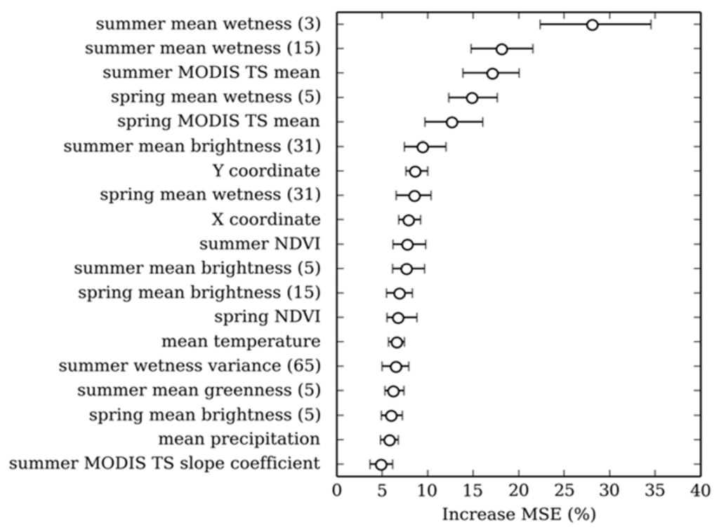
Figure 2. Relative importance of the 18 variables selected for the final random forest model. Confidence intervals (95th percentile) for variable importance were calculated in a bootstrap (N = 50). Increase mean square error (MSE) is the mean of the squared prediction error when the variable is permuted for a random variable [84]. Numbers in brackets indicate the kernel size.

2.3.3. Systematic Error in Model Output

Exploratory analysis suggested a systematic bias in modeled canopy height output, where the height of shorter and taller plots were over and underestimated, respectively. Spatially incorporating an estimate of error (e.g., kriging or cokriging of model residuals) has been utilized previously [20]. However, here this was inappropriate owing to the low spatial autocorrelation in model error (Moran’s I = 0.018, p < 0.001). Alternatively, two aspatial methods were tested to mitigate the systematic bias; (a) resampling of the response variable to a uniform distribution and (b) subtracting from model output a linear model that characterizes the systematic error component. When running random forest as a “classifier”, inequity in class representation can be addressed by either up-sampling or down-sampling the minority and majority classes, respectively [85]. Here a pseudo-uniform distribution for the response variable was computed by aggregating ALS plots into 10 m height cohorts, then using random sampling (with replacement), increasing or decreasing the number of plots in each class accordingly.

For the second approach, a random forest model and a linear model of systematic error were derived from the training dataset, these were then applied to the withheld dataset or across the whole study area. To ensure independence of training and withheld datasets, the training dataset was divided into two halves. The first half of the training data was used to construct the random forest. Linear coefficients were then determined by regressing model residual error, derived from applying the random forest model to the second training dataset, with ALS estimated canopy height. To then estimate canopy height of the withheld dataset (H_RF-SE), the random forest model was applied to the dataset (H_RF) and the systematic component was subtracted as follows:

$$H_{\text{RF}-\text{SE}}= H_{\text{RF}}- \left(\alpha H_{\text{RF}}+\beta \right)$$

(1)

where α and β are the regression coefficients. When applying the technique across the whole study area using the combined random forest model, mean α and β regression coefficients from the cross-validation were used.

3. Results

3.1. Canopy Height Estimation

Cross-validation of random forest for estimating canopy height returned a mean RMSE of 31.3% (5.68 m) at the 95th percentile confidence interval, where the model explained 58% of variance in canopy height (p < 0.0001). Systematic error was apparent in the over and underestimation of shorter and taller canopy heights, respectively (Figure 3A), systematic error accounted for ~2 m of total error. This error was caused by forest plots located towards the tails of the response variable distribution having similar predictor variable values to plots closer to the mean (Figure 4). As a result, canopy height values closer to the mean were preferentially modeled to reduce overall prediction error. For example, plots with a canopy height < 10 m have a comparable spectral response to plots where canopy height is 10–20 m (Figure 4B). As plots in the 10–20 m cohort are more numerous, modeled canopy height for plots where ALS estimated canopy height is < 10 m are allocated to the 10–20 m cohort (Figure 4C). The systematic error resulted in additional kurtosis for modeled canopy height when compared to the distribution of the response variable (compare Figure 4A and C). This effectively reduced the range of canopy height from 1.4–71.9 m for ALS measured canopy height to 7.9–60.7 m for modeled canopy height.

Training random forest with response data that had been resampled to a uniform distribution resulted in a marginal reduction in overall model performance (RMSE = 33% at the 95th percentile confidence interval), however the predicted range of canopy height values increased to 6.7–63.3 m (Figure 3B). When an estimate of systematic error was accounted for the distribution of canopy height closely represents ALS estimate height (Figure 4). Furthermore, the range of canopy height was more representative of the response variable (0.5–68.0 m) and mean error for plots where canopy height was > 50 m and < 10 m were reduced by 4.2 m and 1.2 m, respectively (Figure 4D). Although error became independent of the response variable (Figure 3C), overall model accuracy increased only marginally when compared to the original output (RMSE = 30.4% (6.46 m) at the 95th percentile confidence interval) owing to the rescaling of correctly modeled plots.

A map of canopy height derived from random forest after correcting for the systematic error is presented in Figure 5A. When ALS plots are aggregated into 10 km × 10 km cohorts and compared to the ALS dataset, error was less than ± 15% of ALS derived canopy height for 74% of the study area, less than ± 10% for 57% and less than ± 5% for 33%. Larger errors occur in the taller (south east corner) and shorter (central strip) forests in the study area (Figure 5B and C), which was consistent with the tails of the canopy height distribution being under represented.

Generating a continuous map of canopy height at a 30 m resolution allows for the identification of features in the landscape, for example, caused by land-use and disturbance history. An area of mixed-use forest is presented in Figure 6 where the location, extent and regeneration of (clear-felled) logging coupes are clearly evident. A map generated at a coarser spatial resolution would not identify land-use history with such fidelity. In Figure 6 example A, the poorer model performance for estimating the tails of the canopy height distribution is evident, as it would be expected that canopy height for a recently logged coupe would be closer to 0 m.

Figure 3. ALS derived canopy height (H₉₅) compared to model residual error for random forest models (H_RF); constructed using 5000 ALS plots of untransformed response data (A), 5000 ALS plots where the response variable was resampled to a uniform distribution (B), and subtraction of systematic error from modeled canopy height (C). The coefficient of determination values (r²) were calculated from a linear regression of measured canopy height and model residuals.

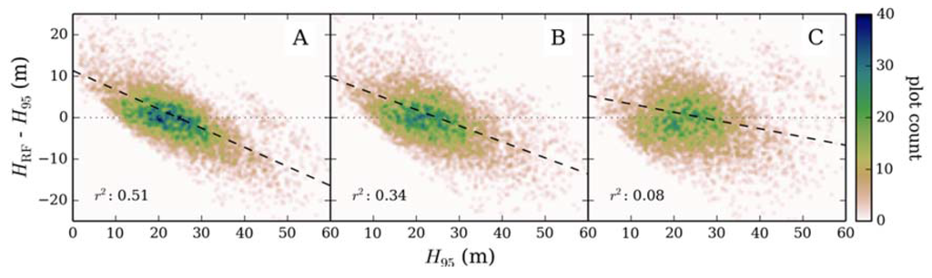
Figure 3. ALS derived canopy height (H₉₅) compared to model residual error for random forest models (H_RF); constructed using 5000 ALS plots of untransformed response data (A), 5000 ALS plots where the response variable was resampled to a uniform distribution (B), and subtraction of systematic error from modeled canopy height (C). The coefficient of determination values (r²) were calculated from a linear regression of measured canopy height and model residuals.

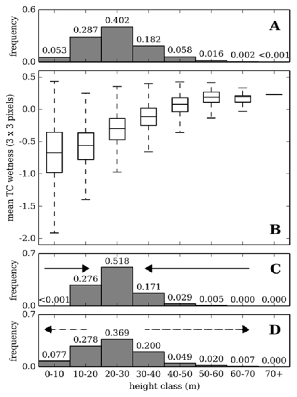
Figure 4. A comparison of the response variable distribution (A), range of Tasselled Cap wetness values (3 × 3 pixels) (B) and the distributions of modeled canopy height (random forest (C) and random forest-systematic error (D)) for different height classes. The solid arrows indicate the direction in which the random forest model output was “squeezed” by inequity in response variable distribution; the dashed arrow indicates the direction canopy height values were rescaled after correcting for systematic error.

Figure 4. A comparison of the response variable distribution (A), range of Tasselled Cap wetness values (3 × 3 pixels) (B) and the distributions of modeled canopy height (random forest (C) and random forest-systematic error (D)) for different height classes. The solid arrows indicate the direction in which the random forest model output was “squeezed” by inequity in response variable distribution; the dashed arrow indicates the direction canopy height values were rescaled after correcting for systematic error.

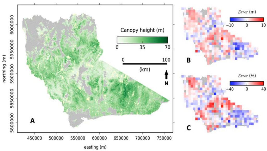
Figure 5. Canopy height at a 30 m resolution (clipped to forest extent) generated using random forest−systematic error (A). Model output when compared to ALS derived canopy height (10 km × 10 km resolution) where error is represented as height difference (B) and percentage of height (C). Coordinate system is the projected Map Grid of Australia (MGA) zone 55.

Figure 5. Canopy height at a 30 m resolution (clipped to forest extent) generated using random forest−systematic error (A). Model output when compared to ALS derived canopy height (10 km × 10 km resolution) where error is represented as height difference (B) and percentage of height (C). Coordinate system is the projected Map Grid of Australia (MGA) zone 55.

3.2. Validation with Inventory Data

Further validation of model output was provided by comparing random forest generated canopy height with forest inventory plots from outside the extent of the ALS capture (Figure 7), the random forest model and random forest minus systematic error returns a RMSE of 29% (5.5 m) and 32% (6.3 m), respectively, at the 95th percentile confidence interval. Although the model output from random forest produces a more accurate result (Figure 7A), correcting for systematic error improved estimates of taller forest inventory plots in particular (Figure 7B). Figure 8 compares ALS and random forest derived canopy height with inventory measurements from within the ALS capture extent. A good statistical association is evident between inventory and ALS measured canopy height where ALS estimates canopy height with a RMSE of 11% (2.9 m). This highlights the suitability of ALS for measuring canopy height over a large area using a single metric, even where forest type is heterogeneous. The association between random forest estimated and inventory measured canopy height is similar to the comparison with forest inventory plots outside the ALS acquisition extent (RMSE = 29% (6.0 m)). Interrogation of the outlier in Figure 8 indicates this was the result of a single emergent tree that was significantly taller than the other trees used to estimate dominant canopy height, thereby increasing the ALS estimate of canopy height.

3.3. Training and Validation of Random Forest Using Smaller Geographic Areas

There was generally no improvement in model performance for random forest trained and validated on smaller geographic areas, when compared to the same area trained using the complete dataset (paired t-test; p = 0.4766). As there is no increase in model performance, this would indicate there is no upper limit to modeled area size, as long as training data captures the variance in canopy height and predictor variables. For some locations a large error (> 10%) was observed from a random forest model trained on a smaller area when compared to the whole area model, this is attributed to a small training dataset (N < 150). Improvements in model performance were seen for an area where mean ALS derived canopy height was 37 m. Taller forests were generally under represented in the study-area wide model (Figure 4), therefore for areas where canopy height was consistently taller a local model yielded improved results.

3.4. Simulating Disparate ALS Capture for Training a Random Forest

When training the model with non-randomly distributed sample points (e.g., simulating aggregation of smaller ALS acquisitions) achievable accuracy reaches an asymptote at ~6% of the total forest area (Figure 9). RMSE and variance in estimates is greater than when compared to a stratified random sample approach. It is suggested that the ~3% increase in RMSE is caused by random forest over-fitting to the training data, therefore extrapolation beyond the training areas is impeded [33]. The large estimate variance is due to the training data either not capturing the variance in the withheld sample (larger error), or the training data and withheld samples having similar canopy height distributions (smaller error). This is exemplified by RMSE of > 40% for a training sample derived from > 90% of the acquisition area (Figure 9), in these instances areas of taller and shorter forest plots were not included in the training cohort.

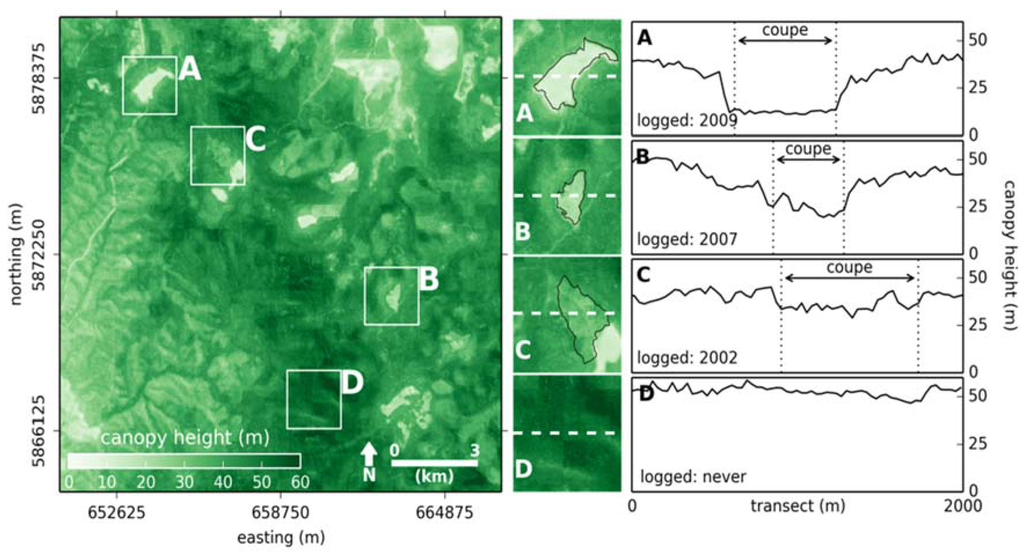
Figure 6. A map of canopy height (30 m resolution) for an area of 16.5 km × 16.5 km, highlighting the land use history of an area of mixed-use forest (left). Three logging coupes that were clear-felled between 2002 and 2009 (A–C) and an area that has never been logged (D) are singled out (coupe extents outlined in black) (center column). Transects of canopy height across each coupe indicating regrowth since logging, coupe boundaries are also identified (right). Coordinate system is the projected Map Grid of Australia (MGA) zone 55.

Figure 6. A map of canopy height (30 m resolution) for an area of 16.5 km × 16.5 km, highlighting the land use history of an area of mixed-use forest (left). Three logging coupes that were clear-felled between 2002 and 2009 (A–C) and an area that has never been logged (D) are singled out (coupe extents outlined in black) (center column). Transects of canopy height across each coupe indicating regrowth since logging, coupe boundaries are also identified (right). Coordinate system is the projected Map Grid of Australia (MGA) zone 55.

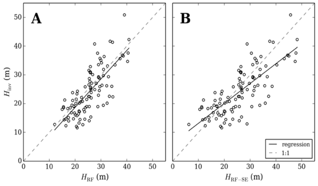
Figure 7. A comparison of inventory measured canopy height (H_inv) with random forest (H_RF) (A) and random forest corrected for systematic error (H_RF-SE) (B) estimated canopy height, at 108 forest inventory plots.

Figure 7. A comparison of inventory measured canopy height (H_inv) with random forest (H_RF) (A) and random forest corrected for systematic error (H_RF-SE) (B) estimated canopy height, at 108 forest inventory plots.

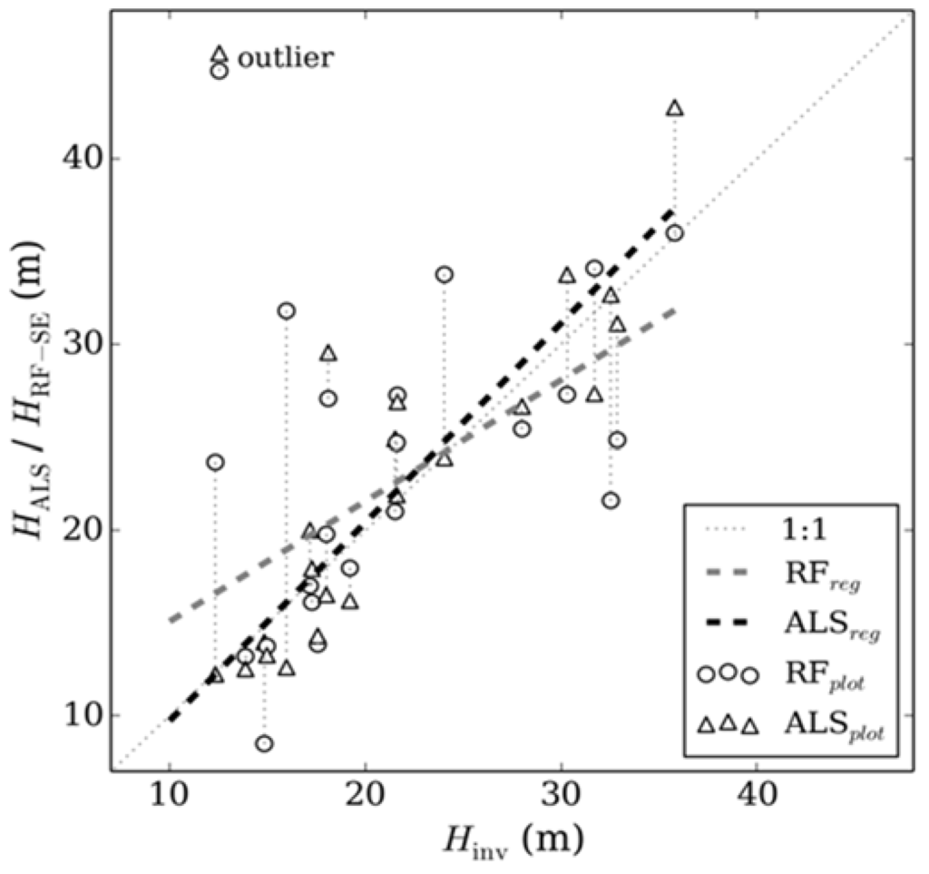
Figure 8. A comparison of inventory (H_inv) measured canopy height and ALS (H_ALS) and random forest-systematic error (H_RF-SE) estimated canopy height, for 22 plots from within the ALS capture area. Vertical dotted lines link the same plot estimated with ALS or random forest.

Figure 8. A comparison of inventory (H_inv) measured canopy height and ALS (H_ALS) and random forest-systematic error (H_RF-SE) estimated canopy height, for 22 plots from within the ALS capture area. Vertical dotted lines link the same plot estimated with ALS or random forest.

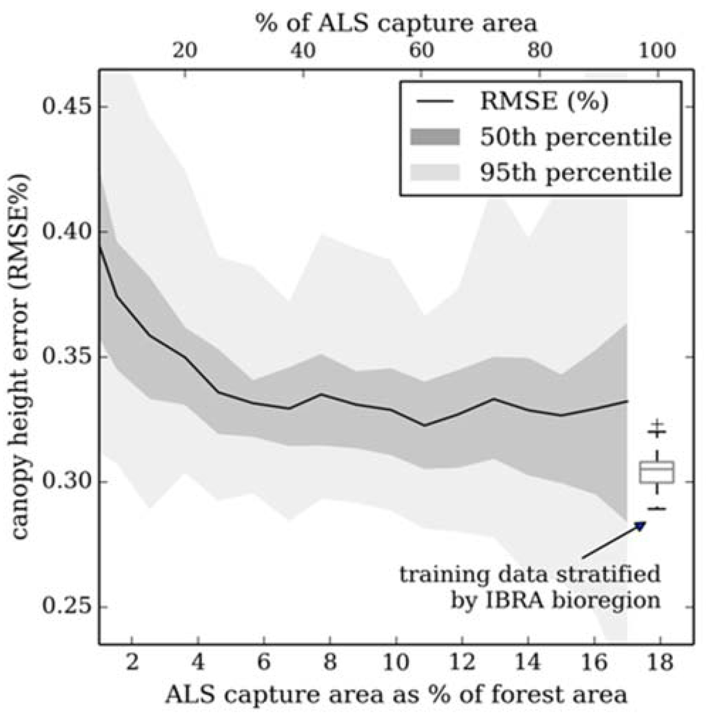
Figure 9. Error in canopy height estimates when constructing random forest models from ALS data selected to represent a combination of a number of disparate (non-random) acquisitions. Model output was validated with ALS plots from outside the training area. For comparison (see boxplot), the results from bootstrapping (N = 50) random forest trained with a random stratified (by IBRA bioregion) sample from across the whole study area (~18% of forested area) is included.

Figure 9. Error in canopy height estimates when constructing random forest models from ALS data selected to represent a combination of a number of disparate (non-random) acquisitions. Model output was validated with ALS plots from outside the training area. For comparison (see boxplot), the results from bootstrapping (N = 50) random forest trained with a random stratified (by IBRA bioregion) sample from across the whole study area (~18% of forested area) is included.

4. Discussion

This manuscript demonstrates a method for assessing canopy height, over a large area, where forest structure is heterogeneous and canopy height ranges from 0–70 m, using freely available predictor data and in an open source computing framework. Forest canopy height was modeled from satellite imagery and ancillary data with a two-stage approach, where ALS data captured over 18% of the study area was used to train the ensemble regression tree model, random forest. Two validation approaches were used, both of which indicate a good agreement between measured and modeled canopy height (RMSE ≤ 31% at the 95th percentile confidence interval). Model error is at the upper limit of acceptable error as stipulated by the European Space Agency (ESA) in the upcoming BIOMASS project when estimating forest biomass from canopy height [86]. However, the ESA target resolution for a canopy height product is much coarser (200 m) than the one presented in this study (30 m).

Previous studies have used regression and machine learning techniques to model canopy height, however these studies have been limited to forests with a maximum canopy height < 30 m or plantations. For example, Mora et al. [19] used high spatial resolution imagery to estimate canopy height for a 7000 ha area of conifer forest, reporting errors of 21% using a k-Nearest Neighbor method. Using a segmented Landsat image to estimate height over 707,000 ha of coniferous forest, Wulder and Seemann [25] reported a standard error of 3.3 m. Applying random forest, Ahmed et al. [38] and Cartus et al. [24] estimated canopy height with an RMSE of ≤ 3.5 m and < 1.7 m for managed coniferous and eucalyptus forests, respectively. When using regression tress to classify plots in height classes ranging from 0 to > 50 m, Peterson and Nelson [41] significantly underestimated canopy height for plots > 50 m when compared to inventory data. A comparison of model output (resampled to 1 km) with the Simard et al. [26] global canopy height product reveals discrepancies between the two approaches of up to ± 20 m over tall and short forest.

The capture or ALS over large areas is still uncommon and previous studies have shown that, over relatively homogeneously forested landscapes, acceptable results can be obtained from a capture of < 1% of the forest area [25]. If a wall-to-wall ALS acquisition is unrealistic, a sample cohort could be created by combining a number of smaller (existing) acquisitions. Results for this study area would suggest that RMSE reaches an asymptote when ALS is acquired over ~6% of forested area. However, a non-random sample returned a larger error when compared to a stratified random sample, even when comprised of plots from over a relatively large area. It is suggested that with a targeted ALS sampling strategy, total area acquired could be reduced. However, this would require detailed a priori knowledge of forest structure or segmentation of a synoptic predictor dataset to infer forest structure variability [87].

Systematic error was apparent in the tails of modeled canopy height distribution, a similar systematic error was evident in other studies that used random forest to model canopy height and biomass [28,39,41]. Two methods were tested to reduce the error; a resampling of the response variable to a uniform distribution and subtracting an estimate of the systematic error component from modeled output. The latter technique proved most successful in recreating the range of canopy heights evident in the training data. However, the transformation is non-discriminate when rescaling canopy height values and therefore inevitably introduced noise to the modeled output (e.g., rescaling values correctly modeled by random forest). This is evident from there being a minimal overall improvement in model performance after subtracting the modeled error component.

Overall, reflectance predictor variables were far more important in the model than other data sources. This would suggest that disturbance has a far bigger influence on determining canopy height than underlying site condition or climatic processes that constrain maximum canopy height. Mascaro et al. [33] found the addition of coordinate variables within the model greatly improved accuracy when estimating biomass, however in this instance this was not the case. The preference of reflectance based model drivers may also indicate that the complex set of environmental variables that limit canopy height are not captured within the datasets used, although the low spatial autocorrelation of model error may suggest otherwise. Furthermore, the resolution of the ancillary datasets were generally much coarser and required resampling, therefore these variables would not have adequately captured the within pixel variance. It should be noted that the specific variables and their relative importance will not be universally applicable across all forests outside of the study area, or in previous or subsequent years [88]. For example, previous and subsequent years would have to be treated as independent and therefore new models created for each [89].

By far the most important variable was the Tasselled Cap (TC) wetness feature, in particular the mean value calculated for a kernel size of 3 × 3 Landsat TM pixels (90 m × 90 m). Calculating a mean value over a kernel, as opposed to individual pixel values, limits the impact of pixel level noise [7]. Variable importance calculated for 50 km × 50 km sub areas, across a wide range of forest types and environmental gradients, also consistently ranked TC wetness as the most important variable. The TC wetness feature is driven by contrast between the visible and infrared and short wave infrared wavelengths, highlighting moisture gradients in a scene [67]. This would indicate that the canopies of taller, denser forests contain more moisture (owing to decreased temperatures and increased evapotranspiration) and shorter forest canopies are more arid, a paradigm that fits the environmental gradients of the study area [57,61]. Previous studies have highlighted the strong association between forest structure and the TC wetness feature [8,22] or middle and short wave infrared wavelengths [28,90]. However, a linear regression of TC wetness (3 × 3 pixels) and canopy height returns a fairly weak statistical association (r² = 0.35), highlighting the requirement for a more complex statistical approach.

Although successful results were obtained, there are a number of potential sources of error worthy of discussion. For example, there is up to two years between ALS and Landsat TM acquisition and up to five years between ALS capture and plot measurements. An assessment of forest inventory plots that have been revisited (a total of 60 state wide) reveals that absolute mean change in canopy height is ~0.5 m per annum. This would suggest that changes in canopy height are minimal at plots that have not been affected by fire or logging in the interim years. Another potential source of error is the limited extent of the ALS capture that was restricted to the riparian zone. Vegetation composition, and therefore structure, is known to differ from non-riparian areas, such as comprising a lower proportion of Eucalypt species [91]. However, ALS transects were the same width along the entire reach of the river and therefore the proportion of riparian vegetation within the sample decreased in the upper catchments. The strong statistical association of forest inventory data from outside the ALS acquisition extent (and therefore away from riparian vegetation) with modeled canopy height would indicate that the impact of the limited sample extent was negligible. The narrow transect width also reduces the number of ALS plots falling within logged coupes or managed plantations, this is a result of a 200 m wide riparian retention strip around all water courses [92]. These management practices are therefore potentially poorly represented in the model e.g., clear-felling in Figure 6.

The analysis presented in this manuscript was achieved using an open source computing framework, in addition, model predictor variables are publically available with a global coverage. Therefore, if training data is available (e.g., canopy height measurements from ALS or forest inventory) the presented methodology could be easily adopted by scientists and land management agencies who wish to map canopy height over large areas. Furthermore, with the planned launch of the Global Ecosystem Dynamics Investigation (GEDI) space borne LiDAR mission in 2018, the opportunity to replace costly ALS or inventory acquisitions with a freely available and spatially continuous sampling method is presented (within the temperate and tropical latitudes) [93].

5. Conclusions

This study presents a method for estimating canopy height at a large-area (i.e., millions of hectares) scale at a 30 m resolution. Application of this method was demonstrated across 2.9 million hectares of heterogeneous forest, comprising a broad range of forest types from open woodland to temperate rainforest, where canopy height ranged from 0–70 m. Canopy height was estimated using a two-stage approach, firstly a random forest ensemble regression tree model was trained with ALS derived canopy height, canopy height estimates were then upscaled to the large area using the synoptic datasets. This was achieved utilizing existing ALS data (i.e., not a bespoke acquisition) in conjunction with synoptic medium resolution freely available satellite imagery (e.g., Landsat Thematic Mapper (TM) and Moderate Resolution Imaging Spectroradiometer). Root mean square error in estimated canopy height was ≤ 31% (~5.6 m) when validated with (a) cross-validation of ALS derived canopy height and (b) a network of forest inventory plots from outside the ALS extent.

Systematic error was evident in model output where taller and shorter forest plots were under and overestimated, respectively. This was corrected for by subtracting an estimate of systematic error, derived from a linear regression of model residuals, from model output. It should be noted that correcting for systematic error did not improve overall model estimates, as plots closer to the mean canopy height were incorrectly rescaled. It is a modelers prerogative whether to estimate broad trends (e.g., using the random forest output) or more accurately attribute outlier values (e.g., subtracting an estimate of systematic error). The model was predominantly driven by reflectance data, in particular the Landsat TM Tasselled Cap transformed wetness feature. This would suggest that in the study area disturbance is the primary constraint on canopy height.

The method framework is designed to be easily adopted by land management agencies. It was shown that the combination of disparate ALS acquisitions (i.e., a non-random sample) covering ~6% of the forested area could be used to successfully estimate canopy height, although results were slightly worse than for a random stratified sample of the entire study area. In the absence of suitable ALS data, the use of forest inventory plot data to train the random forest model is suggested, if the inventory plot network is sufficiently representative. Alternatively, the planned Global Ecosystem Dynamics Investigation (GEDI) space borne LiDAR will offer a near global sampling of forest structure and furthermore will be freely available. This, coupled with the scalability of random forest, suggests application of the technique at a continental or global scale would be entirely feasible.

References

- Wulder, M.A.; White, J.C.; Nelson, R.F.; Næsset, E.; Ørka, H.O.; Coops, N.C.; Hilker, T.; Bater, C.W.; Gobakken, T. LiDAR sampling for large-area forest characterization: A review. Remote Sens. Environ. 2012, 121, 196–209. [Google Scholar] [CrossRef]
- Wulder, M.A.; White, J.C.; Bater, C.W.; Coops, N.C.; Hopkinson, C.; Chen, G. Lidar plots—A new large-area data collection option: Context, concepts, and case study. Can. J. Remote Sens. 2012, 38, 600–618. [Google Scholar] [CrossRef]
- McRoberts, R.E.; Cohen, W.B.; Næsset, E.; Stehman, S.V.; Tomppo, E.O. Using remotely sensed data to construct and assess forest attribute maps and related spatial products. Scand. J. For. Res. 2010, 25, 340–367. [Google Scholar] [CrossRef]
- Wulder, M.A. Optical remote-sensing techniques for the assessment of forest inventory and biophysical parameters. Prog. Phys. Geogr. 1998, 22, 449–476. [Google Scholar] [CrossRef]
- Franklin, J.; Strahler, A.H. Invertible canopy reflectance modeling of vegetation structure in semiarid woodland. IEEE Trans. Geosci. Remote Sens. 1988, 26, 809–825. [Google Scholar] [CrossRef]
- Hansen, M.C.; Potapov, P.V.; Moore, R.; Hancher, M.; Turubanova, S.A.; Tyukavina, A.; Thau, D.; Stehman, S.V.; Goetz, S.J.; Loveland, T.R.; et al. High-resolution global maps of 21st-century forest cover change. Science 2013, 342, 850–853. [Google Scholar] [CrossRef] [PubMed]
- Armston, J.D.; Denham, R.J.; Danaher, T.J.; Scarth, P.; Moffiet, T.N. Prediction and validation of foliage projective cover from Landsat-5 TM and Landsat-7 ETM+ imagery. J. Appl. Remote Sens. 2009. [Google Scholar] [CrossRef]
- Cohen, W.B.; Spies, T.A. Estimating structural attributes of Douglas-fir/western hemlock forest stands from landsat and SPOT imagery. Remote Sens. Environ. 1992, 41, 1–17. [Google Scholar] [CrossRef]
- Lefsky, M.A.; Cohen, W.B.; Parker, G.G.; Harding, D.J. LiDAR remote sensing for ecosystem studies. Bioscience 2002, 52, 19–30. [Google Scholar] [CrossRef]
- Pasher, J.; King, D.J. Development of a forest structural complexity index based on multispectral airborne remote sensing and topographic data This article is one of a selection of papers from extending forest inventory and monitoring over space and time. Can. J. For. Res. 2011, 41, 44–58. [Google Scholar] [CrossRef]
- Holmgren, J.; Jonsson, T. Large scale airborne laser scanning of forest resources in Sweden. Arch. Photogramm. Remote Sens. Spat. Inf. Sic. 2004, 36, 157–160. [Google Scholar]
- Maltamo, M.; Eerikäinen, K.; Packalén, P.; Hyyppä, J. Estimation of stem volume using laser scanning-based canopy height metrics. Forestry 2006, 79, 217–229. [Google Scholar] [CrossRef]
- Torabzadeh, H.; Morsdorf, F.; Schaepman, M.E. Fusion of imaging spectroscopy and airborne laser scanning data for characterization of forest ecosystems—A review. ISPRS J. Photogramm. Remote Sens. 2014, 97, 25–35. [Google Scholar] [CrossRef]
- Quadros, N.; Frisina, R.; Wilson, P. Using airborne survey to map stream Form and Riparian Vegetation Characteristics across Victoria. In Proceedings of the SilviLaser, Hobart, Australia, 16–19 October 2011.
- Asner, G.P.; Powell, G.V.; Mascaro, J.; Knapp, D.E.; Clark, J.K.; Jacobson, J.; Kennedy-Bowdoin, T.; Balaji, A.; Paez-Acosta, G.; Victoria, E.; et al. High-resolution forest carbon stocks and emissions in the Amazon. Proc. Natl. Acad. Sci. 2010, 107, 16738–16742. [Google Scholar] [CrossRef] [PubMed]
- Gregoire, T.G.; Ståhl, G.; Næsset, E.; Gobakken, T.; Nelson, R.F.; Holm, S. Model-assisted estimation of biomass in a LiDAR sample survey in Hedmark County, Norway. Can. J. For. Res. 2011, 41, 83–95. [Google Scholar] [CrossRef]
- Hansen, A.J.; Phillips, L.B.; Dubayah, R.O.; Goetz, S.J.; Hofton, M.A. Regional-scale application of LiDAR: Variation in forest canopy structure across the southeastern US. For. Ecol. Manag. 2014, 329, 214–226. [Google Scholar] [CrossRef]
- Gobakken, T.; Næsset, E.; Nelson, R.; Bollandsås, O.M.; Gregoire, T.G.; Ståhl, G.; Holm, S.; Ørka, H.O.; Astrup, R. Estimating biomass in Hedmark County, Norway using national forest inventory field plots and airborne laser scanning. Remote Sens. Environ. 2012, 123, 443–456. [Google Scholar]
- Mora, B.; Wulder, M.A.; Hobart, G.W.; White, J.C.; Bater, C.W.; Gougeon, F.A.; Varhola, A.; Coops, N.C. Forest inventory stand height estimates from very high spatial resolution satellite imagery calibrated with LiDAR plots. Int. J. Remote Sens. 2013, 34, 4406–4424. [Google Scholar] [CrossRef]
- Hudak, A.T.; Lefsky, M.A.; Cohen, W.B.; Berterretche, M. Integration of LiDAR and Landsat ETM+ data for estimating and mapping forest canopy height. Remote Sens. Environ. 2002, 82, 397–416. [Google Scholar] [CrossRef]
- Ørka, H.O.; Wulder, M.A.; Gobakken, T.; Næsset, E. Integrating airborne laser scanner data and ancillary information for delineating the boreal-alpine transition zone in Hedmark County, Norway. In Proceedings of the SilviLaser 2010, Freiburg, Germany, 14–17 September 2010.
- Pascual, C.; García-Abril, A.; Cohen, W.B.; Martín-Fernández, S. Relationship between LiDAR-derived forest canopy height and Landsat images. Int. J. Remote Sens. 2010, 31, 1261–1280. [Google Scholar] [CrossRef]
- McInerney, D.O.; Suarez-Minguez, J.; Valbuena, R.; Nieuwenhuis, M. Forest canopy height retrieval using LiDAR data, medium-resolution satellite imagery and kNN estimation in Aberfoyle, Scotland. Forestry 2010, 83, 195–206. [Google Scholar] [CrossRef]
- Cartus, O.; Kellndorfer, J.M.; Rombach, M.; Walker, W. Mapping canopy height and growing stock volume using airborne LiDAR, ALOS PALSAR and Landsat ETM+. Remote Sens. 2012, 4, 3320–3345. [Google Scholar] [CrossRef]
- Wulder, M.A.; Seemann, D. Forest inventory height update through the integration of LiDAR data with segmented Landsat imagery. Can. J. Remote Sens. 2003, 29, 536–543. [Google Scholar] [CrossRef]
- Simard, M.; Pinto, N.; Fisher, J.B.; Baccini, A. Mapping forest canopy height globally with spaceborne LiDAR. J. Geophys. Res. 2011, 116, 1–12. [Google Scholar] [CrossRef]
- Lefsky, M.A. A global forest canopy height map from the Moderate Resolution Imaging Spectroradiometer and the Geoscience Laser Altimeter System. Geophys. Res. Lett. 2010, 37, 1–5. [Google Scholar] [CrossRef]
- Baccini, A.; Laporte, N.T.T.; Goetz, S.J.; Sun, M.; Dong, H. A first map of tropical Africa’s above-ground biomass derived from satellite imagery. Environ. Res. Lett. 2008, 3, 1–9. [Google Scholar] [CrossRef]
- Mellor, A.; Haywood, A.; Stone, C.; Jones, S. The performance of random forests in an operational setting for large area sclerophyll forest classification. Remote Sens. 2013, 5, 2838–2856. [Google Scholar] [CrossRef]
- Breiman, L. Random forests. Mach. Learn. 2001, 45, 5–32. [Google Scholar] [CrossRef]
- Breiman, L. Bagging predictors. Mach. Learn. 1996, 24, 123–140. [Google Scholar] [CrossRef]
- Rodriguez-Galiano, V.F.; Ghimire, B.; Rogan, J.; Chica-Olmo, M.; Rigol-Sanchez, J.P. An assessment of the effectiveness of a random forest classifier for land-cover classification. ISPRS J. Photogramm. Remote Sens. 2012, 67, 93–104. [Google Scholar] [CrossRef]
- Mascaro, J.; Asner, G.P.; Knapp, D.E.; Kennedy-Bowdoin, T.; Martin, R.E.; Anderson, C.; Higgins, M.; Chadwick, K.D. A tale of two “Forests”: Random Forest machine learning aids tropical Forest carbon mapping. PLoS ONE 2014, 9, 12–16. [Google Scholar] [CrossRef] [PubMed]
- Evans, J.S.; Cushman, S.A. Gradient modeling of conifer species using random forests. Landscape. Ecol. 2009, 24, 673–683. [Google Scholar] [CrossRef]
- Mellor, A.; Jones, S.D.; Haywood, A.; Wilkes, P. Using random forest decision tree classification for large area forest extent mapping with multi-source remote sensing and GIS data. In Proceedings of the 16th Australasian Remote Sensing and Photogrammetry Conference, Melbourne, Australia, 27–28 August 2012.
- Mellor, A.; Boukir, S.; Haywood, A.; Jones, S. Exploring issues of training data imbalance and mislabelling on random forest performance for large area land cover classification using the ensemble margin. ISPRS J. Photogramm. Remote Sens. 2015, 105, 155–168. [Google Scholar] [CrossRef]
- Johansen, K.; Phinn, S.; Witte, C. Mapping of riparian zone attributes using discrete return LiDAR, QuickBird and SPOT-5 imagery: Assessing accuracy and costs. Remote Sens. Environ. 2010, 114, 2679–2691. [Google Scholar] [CrossRef]
- Ahmed, O.S.; Franklin, S.E.; Wulder, M.A.; White, J.C. Characterizing stand-level forest canopy cover and height using Landsat time series, samples of airborne LiDAR, and the random forest algorithm. ISPRS J. Photogramm. Remote Sens. 2015, 101, 89–101. [Google Scholar] [CrossRef]
- Kellndorfer, J.M.; Walker, W.S.; LaPoint, E.; Kirsch, K.; Bishop, J.; Fiske, G. Statistical fusion of LiDAR, InSAR, and optical remote sensing data for forest stand height characterization: A regional-scale method based on LVIS, SRTM, Landsat ETM+, and ancillary data sets. J. Geophys. Res. Biogeosci. 2010. [Google Scholar] [CrossRef]
- Stojanova, D.; Panov, P.; Gjorgjioski, V.; Kobler, A.; Džeroski, S. Estimating vegetation height and canopy cover from remotely sensed data with machine learning. Ecol. Inform. 2010, 5, 256–266. [Google Scholar] [CrossRef]
- Peterson, B.; Nelson, K. Mapping forest height in Alaska using GLAS, Landsat composites, and airborne LiDAR. Remote Sens. 2014, 6, 12409–12426. [Google Scholar] [CrossRef]
- Turner, W.; Rondinini, C.; Pettorelli, N.; Mora, B.; Leidner, A.K.; Szantoi, Z.; Buchanan, G.; Dech, S.; Dwyer, J.; Herold, M.; et al. Free and open-access satellite data are key to biodiversity conservation. Biol. Conserv. 2015, 182, 173–176. [Google Scholar] [CrossRef]
- Rodriguez-Galiano, V.F.; Chica-Olmo, M.; Abarca-Hernandez, F.; Atkinson, P.M.; Jeganathan, C. Random forest classification of mediterranean land cover using multi-seasonal imagery and multi-seasonal texture. Remote Sens. Environ. 2012, 121, 93–107. [Google Scholar] [CrossRef]
- Coburn, C.; Roberts, A. A multiscale texture analysis procedure for improved forest stand classification. Int. J. Remote Sens. 2004, 25, 4287–4308. [Google Scholar] [CrossRef]
- Ghimire, B.; Rogan, J.; Miller, J. Contextual land-cover classification: incorporating spatial dependence in land-cover classification models using random forests and the Getis statistic. Remote Sens. Lett. 2010, 1, 45–54. [Google Scholar] [CrossRef]
- Franklin, S.E.; Wulder, M.A.; Gerylo, G.R. Texture analysis of IKONOS panchromatic data for Douglas-fir forest age class separability in British Columbia. Int. J. Remote Sens. 2001, 22, 2627–2632. [Google Scholar] [CrossRef]
- Lefsky, M.A.; Cohen, W.B.; Harding, D.J. LiDAR remote sensing of above ground biomass in three biomes. Int. Arch. Photogramm. Remote Sens. 2001, 34, 155–162. [Google Scholar] [CrossRef]
- Lucas, R.M.; Lee, A.C.; Bunting, P.J. Retrieving forest biomass through integration of CASI and LiDAR data. Int. J. Remote Sens. 2008, 29, 1553–1577. [Google Scholar] [CrossRef]
- Goetz, S.J.; Steinberg, D.; Dubayah, R.O.; Blair, B.J. Laser remote sensing of canopy habitat heterogeneity as a predictor of bird species richness in an eastern temperate forest, USA. Remote Sens. Environ. 2007, 108, 254–263. [Google Scholar] [CrossRef]
- Hyde, P.; Dubayah, R.O.; Walker, W.; Blair, B.J.; Hofton, M.A.; Hunsaker, C. Mapping forest structure for wildlife habitat analysis using multi-sensor (LiDAR, SAR/InSAR, ETM+, Quickbird) synergy. Remote Sens. Environ. 2006, 102, 63–73. [Google Scholar] [CrossRef]
- Næsset, E. Airborne laser scanning as a method in operational forest inventory: Status of accuracy assessments accomplished in Scandinavia. Scand. J. For. Res. 2007, 22, 433–442. [Google Scholar] [CrossRef]
- Næsset, E. Determination of mean tree height of forest stands using airborne laser scanner data. ISPRS J. Photogramm. Remote Sens. 1997, 52, 49–56. [Google Scholar] [CrossRef]
- Wulder, M.A.; Bater, C.W.; Coops, N.C.; Hilker, T.; White, J.C. The role of LiDAR in sustainable forest management. For. Chron. 2008, 84, 807–826. [Google Scholar] [CrossRef]
- Miles, P.D. Using biological criteria and indicators to address forest inventory data at the state level. For. Ecol. Manag. 2002, 155, 171–185. [Google Scholar] [CrossRef]
- National Forest Inventory. Australia’s State of the Forests Report 1998; National Forest Inventory, Bureau of Rural Sciences: Canberra, Australia, 1998.
- Department of Environment Australia’s bioregions (IBRA). Available online: http://www.environment.gov.au/land/nrs/science/ibra (accessed on 29 July 2015).
- Gellie, N.J.H. Native vegetation of the Southern Forests: South-east highlands, Australian alps, south-west slopes, and SE corner bioregions. Cunninghamia 2005, 9, 219–254. [Google Scholar]
- Van Dijk, A.I.J.M.; Beck, H.E.; Crosbie, R.S.; de Jeu, R.A.M.; Liu, Y.Y.; Podger, G.M.; Timbal, B.; Viney, N.R. The Millennium Drought in southeast Australia (2001–2009): Natural and human causes and implications for water resources, ecosystems, economy, and society. Water Resour. Res. 2013, 49, 1040–1057. [Google Scholar] [CrossRef]
- Semple, B.; Rankin, M.; Koen, T.; Geeves, G. A note on tree deaths during the current (2001–?) drought in South-eastern Australia. Aust. Geogr. 2010, 41, 391–401. [Google Scholar] [CrossRef]
- Jacobs, M.R. Growth Habits of the Eucalypts; Commonwealth Forestry and Timber Bureau: Canberra, Australia, 1955. [Google Scholar]
- Jenkins, R.B.; Coops, N.C. Landscape controls on structural variation in Eucalypt vegetation communities: Woronora Plateau, Australia. Aust. Geogr. 2011, 42, 1–17. [Google Scholar] [CrossRef]
- Department of Sustainability and Environment Victorian Forest Monitoring Program Guidelines for Ground Plot Measurement Standard Operating Procedure 13: Measuring a Large Tree Plot. Available online: http://www.depi.vic.gov.au/__data/assets/pdf_file/0013/226030/SOP13_v1.2.pdf (accessed on 29 July 2015).
- Lovell, J.L.; Jupp, D.L.; Culvenor, D.S.; Coops, N.C. Using airborne and ground-based ranging Lidar to measure canopy structure in Australian forests. Can. J. Remote Sens. 2003, 29, 607–622. [Google Scholar] [CrossRef]
- Wilkes, P.; Jones, S.D.; Suarez, L.; Haywood, A.; Mellor, A.; Woodgate, W.; Soto-berelov, M.; Skidmore, A.K. Understanding the effects of ALS pulse density for metric retrieval across diverse forest types. Photogramm. Eng. Remote Sens. 2015, 81, 625–635. [Google Scholar] [CrossRef]
- LAStools-Efficient Tools for LiDAR Processing 2012. Available online: http://rapidlasso.com/lastools/ (accessed 18 September 2015).
- Flood, N.; Danaher, T.; Gill, T.; Gillingham, S. An operational scheme for deriving standardised surface reflectance from landsat TM/ETM+ and SPOT HRG imagery for Eastern Australia. Remote Sens. 2013, 5, 83–109. [Google Scholar] [CrossRef]
- Crist, E.P.; Cicone, R.C. A physically-based transformation of Thematic Mapper data—The TM Tasseled Cap. IEEE Trans. Geosci. Remote Sens. 1984, 3, 256–263. [Google Scholar] [CrossRef]
- Wilkes, P.; Jones, S.D.; Suarez, L.; Haywood, A.; Mellor, A.; Woodgate, W.; Soto-Berelov, M.; Skidmore, A.K. Using discrete-return ALS to quantify number of canopy strata across diverse forest types. Methods Ecol. Evol. 2015, in press. [Google Scholar]
- Zhang, X.; Friedl, M.A.; Schaaf, C.B.; Strahler, A.H.; Hodges, J.C.F.; Gao, F.; Reed, B.C.; Huete, A. Monitoring vegetation phenology using MODIS. Remote Sens. Environ. 2003, 84, 471–475. [Google Scholar] [CrossRef]
- Austin, M.P. Models for the analysis of species’ response to environmental gradients. Vegetatio 1987, 69, 35–45. [Google Scholar] [CrossRef]
- Hijmans, R.J.; Cameron, S.E.; Parra, J.L.; Jones, P.G.; Jarvis, A. Very high resolution interpolated climate surfaces for global land areas. Int. J. Climatol. 2005, 25, 1965–1978. [Google Scholar] [CrossRef]
- Global Soil Water Balance Geospatial Database. CGIAR Consortium for Spatial Information. Available online: http://www.cgiar-csi.org (accessed on 29 July 2015).
- National Resource Information Centre Atlas of Australian Soils (digital version). Available online: http://gcmd.gsfc.nasa.gov/KeywordSearch/Metadata.do?Portal=idn_ceos&KeywordPath=[Keyword%3D%27NORTHCOTE+CLASSIFICATION%27]&EntryId=EARTH_LAND_AUS_NRIC_SOILS1&MetadataView=Full&MetadataType=0&lbnode=mdlb4 (accessed on 29 July 2015).
- McGarigal, K.; Tagil, S.; Cushman, S.A. Surface metrics: An alternative to patch metrics for the quantification of landscape structure. Landscape Ecol. 2009, 24, 433–450. [Google Scholar] [CrossRef]
- Lindenmayer, D.B.; Cunningham, R.; Donnelly, C.; Franklin, J.F. Structural features of old-growth Australian montane ash forests. For. Ecol. Manag. 2000, 134, 189–204. [Google Scholar] [CrossRef]
- ForestLAS Python packakge 2015. Available online: https://bitbucket.org/phil_wilkes/forestlas (accessed 18 September 2015).
- GRASS Development Team Geographic Resources Analysis Support System (GRASS) Software 2015. Available online: https://grass.osgeo.org (accessed on 29 July 2015).
- QGIS Development Team QGIS Geographic Information System. Open Source Geospatial Foundation Project 2015. Available online: http://www.qgis.org/en/site/ (accessed on 29 July 2015).
- Python Software Foundation Python 2015. Available online: https://www.python.org/psf-landing/ (accessed on 29 July 2015).
- R Development Core Team R: A Language and Environment for Statistical Computing 2014. Available online: http://www.R-project.org (accessed on 29 July 2015).
- Liaw, A.; Wiener, M. Package “randomForest”. 2013. Available online: https://cran.r-project.org/web/packages/RRF/RRF.pdf (accessed on 29 July 2015).
- Murphy, M.A.; Evans, J.S.; Strofer, A. Quantifying Bufo boreas connectivity in Yellowstone National Park with landscape genetics. Ecology 2010, 91, 252–261. [Google Scholar] [CrossRef] [PubMed]
- Svetnik, V.; Liaw, A.; Tong, C.; Wang, T. Application of Breiman’s random forest to modeling structure-activity relationships of pharmaceutical molecules. Mult. Classif. Syst. 2004. [Google Scholar] [CrossRef]
- Cutler, D.R.; Edwards, T.J.; Beard, K.; Cutler, A.; Hess, K.T.; Gibson, J.; Lawler, J.J. Random forests for classification in ecology. Ecology 2007, 88, 2783–2792. [Google Scholar] [CrossRef] [PubMed]
- Using Random Forest to Learn Imbalanced Data. Available online: http://statistics.berkeley.edu/sites/default/files/tech-reports/666.pdf (accessed on 29 July 2015).
- Seifert, F.; Scipal, K.; Quegan, S.; Le Toan, T. The Earth Explorer Biomass Mission—Status and preparatory activities. In Proceedings of the GOFC/GOLD Biomass workshop, Brisbane, Australia, 24–26 February 2015.
- McRoberts, R.E.; Tomppo, E.O. Remote sensing support for national forest inventories. Remote Sens. Environ. 2007, 110, 412–419. [Google Scholar] [CrossRef]
- Foody, G.M.; Boyd, D.S.; Cutler, M.E. Predictive relations of tropical forest biomass from Landsat TM data and their transferability between regions. Remote Sens. Environ. 2003, 85, 463–474. [Google Scholar] [CrossRef]
- Hudak, A.T.; Strand, E.K.; Vierling, L.A.; Byrne, J.C.; Eitel, J.U.; Martinuzzi, S.; Falkowski, M.J. Quantifying aboveground forest carbon pools and fluxes from repeat LiDAR surveys. Remote Sens. Environ. 2012, 123, 25–40. [Google Scholar] [CrossRef]
- Steininger, M.K. Satellite estimation of tropical secondary forest above-ground biomass: Data from Brazil and Bolivia. Int. J. Remote Sens. 2000, 21, 1139–1157. [Google Scholar] [CrossRef]
- Lindenmayer, D.B. Factors at multiple scales affecting distribution patterns and their implications for animal conservation—Leadbeater’s Possum as a case study. Biodivers. Conserv. 2000, 9, 15–35. [Google Scholar] [CrossRef]
- VicForests Operating Procedures Regulatory Handbook Version 2.1. 2014. Available online: www.vicforests.com.au/files/dbkixdmfrz/VicForests-Operating-Procedures---Regulatory-Handbook-v2.1.pdf (accessed on 29 July 2015).
- Dubayah, R.O.; Schaaf, C.B. Global ecosystem dynamics investigation. In Proceedings of the GOFC/GOLD Biomass workshop, Brisbane, Australia, 24–26 February 2015.
© 2015 by the authors; licensee MDPI, Basel, Switzerland. This article is an open access article distributed under the terms and conditions of the Creative Commons Attribution license (http://creativecommons.org/licenses/by/4.0/).