Rooftop Surface Temperature Analysis in an Urban Residential Environment

Abstract

The urban heat island (UHI) phenomenon is a significant worldwide problem caused by rapid population growth and associated urbanization. The UHI effect exacerbates heat waves during the summer, increases energy and water consumption, and causes the high risk of heat-related morbidity and mortality. UHI mitigation efforts have increasingly relied on wisely designing the urban residential environment such as using high albedo rooftops, green rooftops, and planting trees and shrubs to provide canopy coverage and shading. Thus, strategically designed residential rooftops and their surrounding landscaping have the potential to translate into significant energy, long-term cost savings, and health benefits. Rooftop albedo, material, color, area, slope, height, aspect and nearby landscaping are factors that potentially contribute. To extract, derive, and analyze these rooftop parameters and outdoor landscaping information, high resolution optical satellite imagery, LIDAR (light detection and ranging) point clouds and thermal imagery are necessary. Using data from the City of Tempe AZ (a 2010 population of 160,000 people), we extracted residential rooftop footprints and rooftop configuration parameters from airborne LIDAR point clouds and QuickBird satellite imagery (2.4 m spatial resolution imagery). Those parameters were analyzed against surface temperature data from the MODIS/ASTER airborne simulator (MASTER). MASTER images provided fine resolution (7 m) surface temperature data for residential areas during daytime and night time. Utilizing these data, ordinary least squares (OLS) regression was used to evaluate the relationships between residential building rooftops and their surface temperature in urban environment. The results showed that daytime rooftop temperature was closely related to rooftop spectral attributes, aspect, slope, and surrounding trees. Night time temperature was only influenced by rooftop spectral attributes and slope.

1. Introduction

Today, 54% of the world’s population live in urban areas, and estimates indicate that the urban population will increase to 66% by 2050 [1]. This population surge will require rapid transformation of undeveloped land into urban uses. The modification of the earth’s surface to urban has resulted in higher temperatures in urban environments compared to surrounding rural environments, a well-known phenomenon commonly referred to as the urban heat island (UHI) effect [2,3,4]. The UHI exacerbates heat waves during the summer, increases energy consumption, and more importantly elevates the risk of heat-related morbidity and mortality, especially for the elderly, young children, and low-income residents, who are more vulnerable to excessive heat stress due to a variety of physical, social, and economic reasons [5,6,7,8,9]. Many existing studies have made attempts to understand and mitigate UHI effect in major cities all over the world, such as London, Beijing, Paris, Shanghai, Hong Kong, and Moscow [10,11,12,13,14,15,16]. UHI mitigation via sustainable design of the urban environment has received increasing attention from ecologists, urban planners, and policymakers. Commonly practiced mitigation strategies include but are not limited to: increasing number of parks and coverage of green space near residential areas [17,18,19,20], installing green roofs or other cool roofs built with high-albedo materials [21,22,23,24], using cold pavement materials [25,26,27], and creating better urban design for air flow [28]. The goal of this paper is to use remotely sensed imagery and data processing to evaluate the contribution of residential rooftop properties and nearby vegetation in understanding urban heat.

Remote sensing continues to contribute to detecting and understanding the interplay between urban land covers and urban heat [29,30,31,32]. While little research takes place at the single-building level, recent contributions highlight the importance of not just of the urban surface materials but the density, juxtaposition, and pattern of land features [33,34,35]. Using datasets such as ASTER, Quickbird, and Landsat ETM+, researchers show that proximity to asphalt surfaces and dark roofs and the pattern of impervious surfaces increase land surface temperature and denser nearby vegetation cools surfaces [36,37]. For cooling urban areas, Fan and Myint [38] examined the utility of spatial autocorrelation indices in characterizing spatial arrangement of urban landscape at the class- and landscape- levels, and reported the aggregate cooling effect of clustered vegetation patches compared to dispersed and fragmented patterns [39]. Maimaitiyiming et al. [40] analyzed the relationships between the UHI effects and green spaces configuration through TM thermal infrared imagery finding that increasing edge density of the green space can improve the urban thermal environment.

For individual structures, cooler micro-climates due to the presence and proximity of parks and green spaces can offer UHI mitigation [41]. Myint et al. [42] showed that dense vegetation cover within an area from 210 m × 210 m to 270 m × 270 m decreased the maximum air temperature. Tree canopy cover and tree shade serve as a natural umbrella to decrease insolation and reduce air and surface temperatures [43]. Strategic planning of trees has the potential to provide significant energy and long-term cost savings, enhance the urban ecosystem, and promote a range of human health benefits [44,45,46,47].

While proximity to parks and green spaces is vital in cooling residential neighborhoods, the cooling effects of green roofs, cool roofs, and green space on urban microclimate is also central to UHI mitigation [18,21,33,48,49]. To reduce rooftop surface temperatures, green roof (vegetation cover) and reflective roof (high albedo rooftop materials) are two primary materials to create “UHI-ameliorated” roofs. Thus, shifting to high albedo rooftops, rooftop gardens, or green roofs potentially helps reduce UHI effect for individual structures [21,24,49,50,51,52]. Akbari et al. [22] discussed the cooling energy savings of high-albedo rooftops during peak power in a house and a school in Sacramento, California. The relationships between rooftop albedo and surface temperature were further analyzed. High albedo rooftops reduced the amount of solar radiation absorbed by urban structures and building envelopes and decreased the surface temperature [53]. A well-performing high albedo coatings were able to save up to 70% of the energy for residential buildings [54]. However, few researchers utilize remote sensing to deal with individual building structures in understanding UHI mitigation. The main challenge in using remotely sensed data for structure-based analysis is that most available thermal imagery (e.g., ASTER thermal at 90 m and Landsat 8 TIR imagery at 100 m) fail to offer fine-resolution spatial details at the structure level. Meanwhile, rooftops are the major imperious surfaces in the urban residential environment and it is important to quantify the relationships between land surface temperature, rooftop configuration, and geophysical characteristics. There remains a challenge to effectively and accurately evaluate the impact of rooftop surface temperatures through thermal remotely sensed imagery.

Understanding the relationship between microclimates and small area urban features is now possible due to the availability of higher spatial resolution thermal images, an important contribution to understanding UHI mitigation strategies. MASTER imagery, with seven-meter spatial resolution thermal bands, is a significant improvement over Landsat 8 and ASTER. With the MASTER imagery, it is possible to analyze the land cover types at a large scale such as rooftops, tree canopies, and pavement. At the same time, existing multi-spectral high spatial-resolution satellite imagery such as QuickBird (2.4 m) and IKONOS (4 m) or aerial photogrammetry create the possibility to delineate roof boundaries [55,56,57], and provide an efficient and cost-effective means to capture roof albedo in a large area. Airborne LIDAR (light detection and ranging) point clouds provide highly accurate building height information for roof parameter extraction [58,59]. These make the detailed rooftop temperature analysis based on rooftop configuration and geophysical properties feasible and executable.

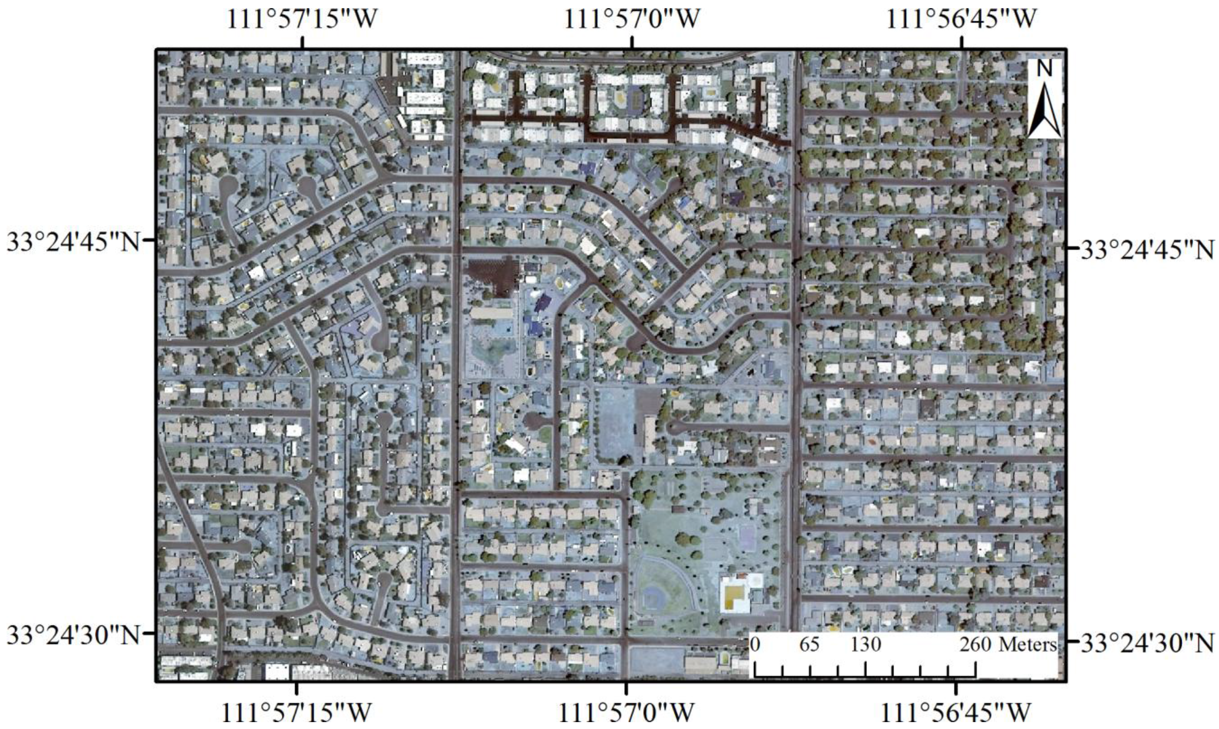
The goal of this study is to explore the relationships between rooftop surface temperature, rooftop geophysical parameters, rooftop configuration, and nearby landscaping through QuickBird, MASTER and LIDAR imagery. In particular, we investigate the urban residential area in Tempe, Arizona, U.S.A. This study will explore the relationships among buildings, trees, and UHI effects, and attempt to better understand the inner-connection of rooftops and the UHI effect.

2. Study Area and Data

2.1. Study Area

This study focuses on a residential neighborhood with detached single-family houses in the City of Tempe, Arizona (Figure 1). The City of Tempe is a municipality in the greater Phoenix metropolitan area located in the northern part of the Sonoran Desert in the U.S. Southwest. With summertime temperatures reaching or exceeding 43 °C, heat mitigation strategies are mandatory, including private pools, outdoor green landscaping, and central air conditioning. The population of Tempe reached 160,000 by 2010 with the majority living in single-family detached dwellings [60]. We focused on 567 single family detached homes built during the 1950s and 1960s. All of the houses are single story with sizes from 76 m² to 457 m² with a mean and standard deviation of 134 m² and 31 m² respectively, according to the Maricopa County Assessor’s records. Parcel size ranges from 640 m² to 1725 m² with a mean of 695 m² and standard deviation of 138 m². The neighborhood does not have a home owner’s association (HOA) so there are no regulations mandating front yard landscaping. In spite of this, 95% of the neighborhood has trees in their yards, offering some level of tree shade to the home structures.

Figure 1. Study area.

Figure 1. Study area.

2.2. Data

To extract rooftop parameters, several remotely sensed data sources were used. The data sources used for land use/cover classification were QuickBird imagery and high-resolution airborne LIDAR data. MODIS/ASTER airborne simulator imagery provided the thermal information of rooftops. National Agriculture Imagery Program imagery and Bing Map served as reference imagery. The average value of the rooftop temperature, rooftop configuration parameters, and albedo/reflectance for each entire rooftop were derived from these sources.

Figure 2. Airborne LIDAR point clouds.

Figure 2. Airborne LIDAR point clouds.

Figure 3. Raw MASTER daytime imagery.

Figure 3. Raw MASTER daytime imagery.

The QuickBird satellite imagery was collected on 30 March 2008 with four-band pan sharpening with 2.4 m resolution multispectral (Base map of Figure 1). The LIDAR data obtained on 5 May 2008 contain elevation data with a 95% vertical accuracy of 18.5 cm and a 90% of 15 cm with horizontal accuracy of 30 cm, 1 sigma (Figure 2). MODIS/ASTER airborne simulator imagery (7 m spatial resolution) developed by NASA [61] was collected over the Phoenix metropolitan area on 12 July (daytime, Figure 3) and 15 July (night time, Figure 4), 2011. MASTER imagery was acquired over the visible through mid-infrared wavelengths (0.46–12.817 μm) in 50 spectral bands. Surface emissivity was obtained from the mid-infrared bands (bands 41–50) and was used for surface energy balance and fine-scale surface temperature analysis. National Agriculture Imagery Program (NAIP, 1 m/pixel, 2010) imagery was employed as reference data for MASTER image registration because it had the most similar pixel size and featured discrimination for tie-pointing to the MASTER data (Figure 5). A second order polynomial transformation was used to obtain a better co-registration accuracy. Bing Map was used to manually digitize the building rooftop footprints (Rooftop boundaries shown in Figure 1). 567 rooftop footprints were manually digitized for our study area. Rooftop boundaries that were obscured by vegetation were extrapolated to a rectangular shape based on visible rooftop boundaries.

Figure 4. Raw MASTER night time imagery.

Figure 4. Raw MASTER night time imagery.

Figure 5. NAIP imagery.

Figure 5. NAIP imagery.

3. Methods

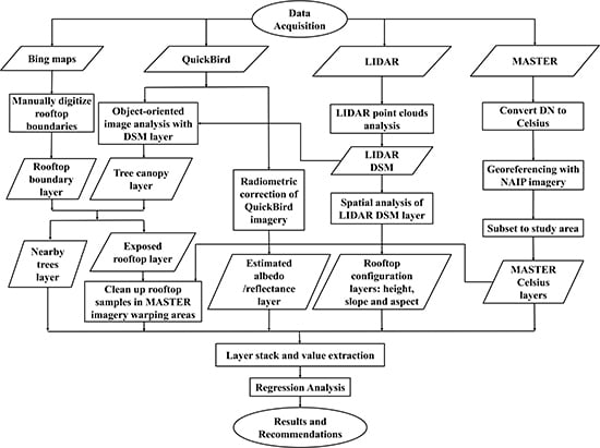
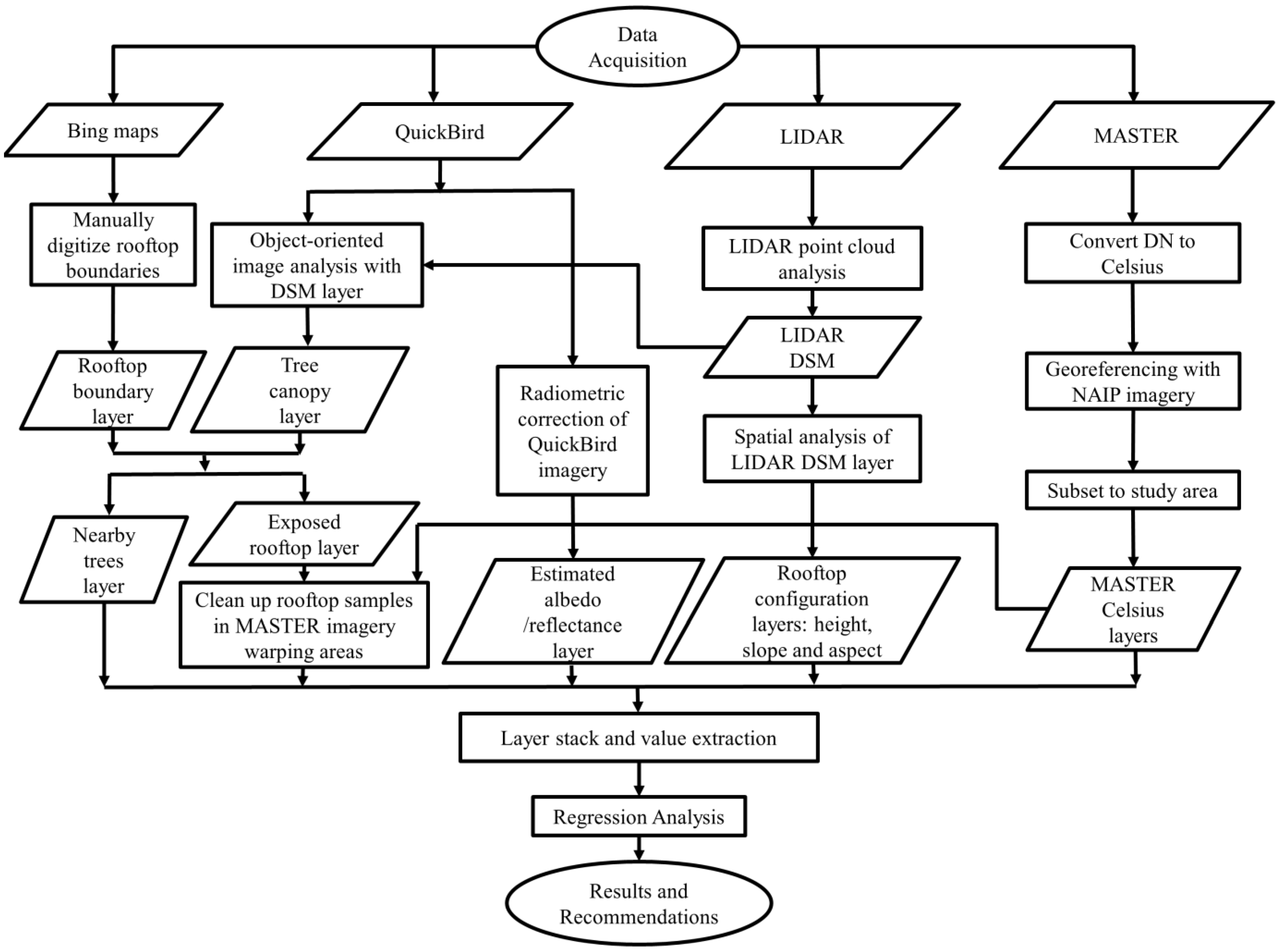
The methodology consists of remote sensing data processing, calculation of derivative rooftop parameters, and regression modeling. The methodological framework is shown in Figure 6 and described in detail in this section.

Figure 6. Methodology framework (QuickBird image classification, LIDAR point clouds analysis and atmospheric and geometric correction of MASTER imagery).

Figure 6. Methodology framework (QuickBird image classification, LIDAR point clouds analysis and atmospheric and geometric correction of MASTER imagery).

3.1. Image Processing and Surrounding Trees Extraction

3.1.1. LIDAR Point Clouds Processing

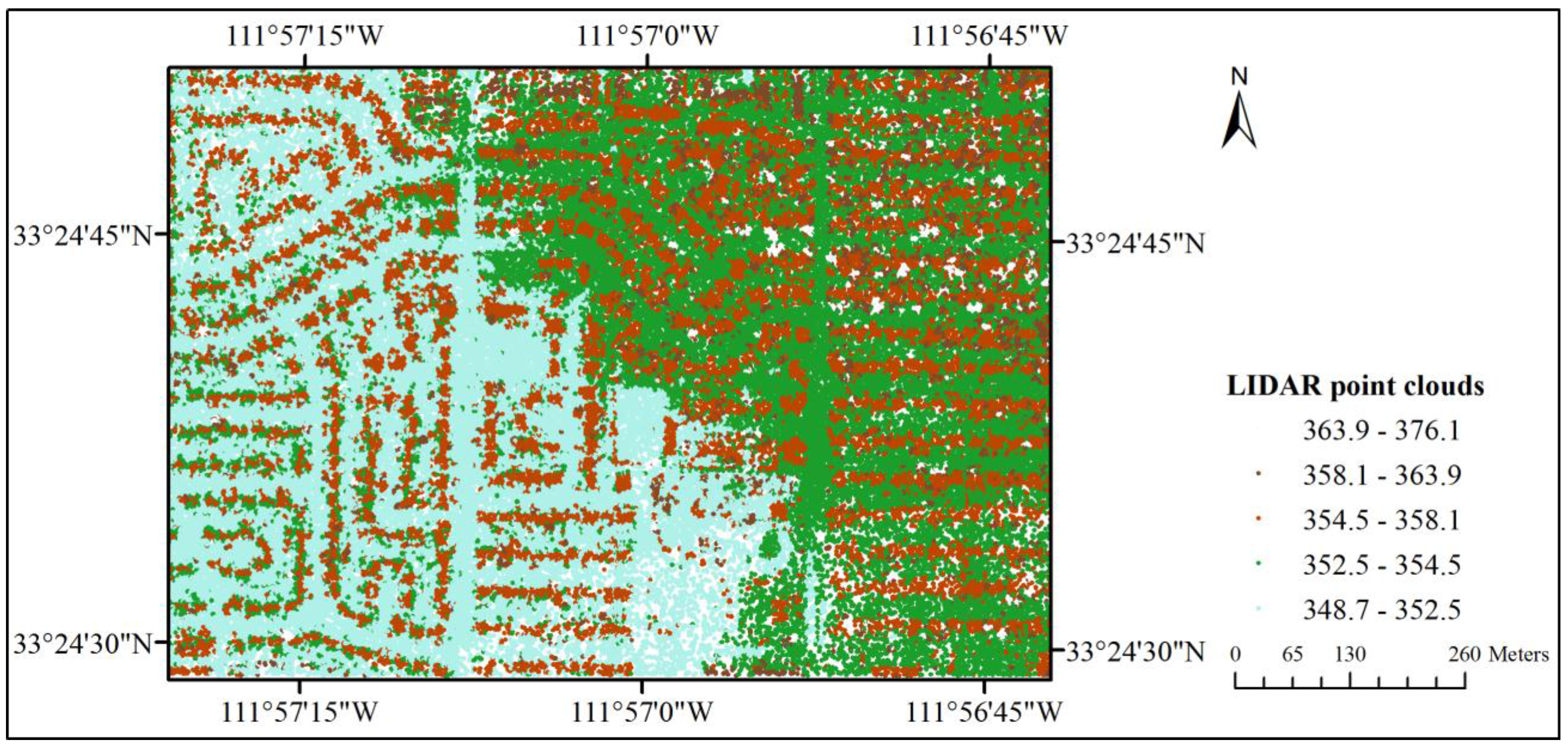
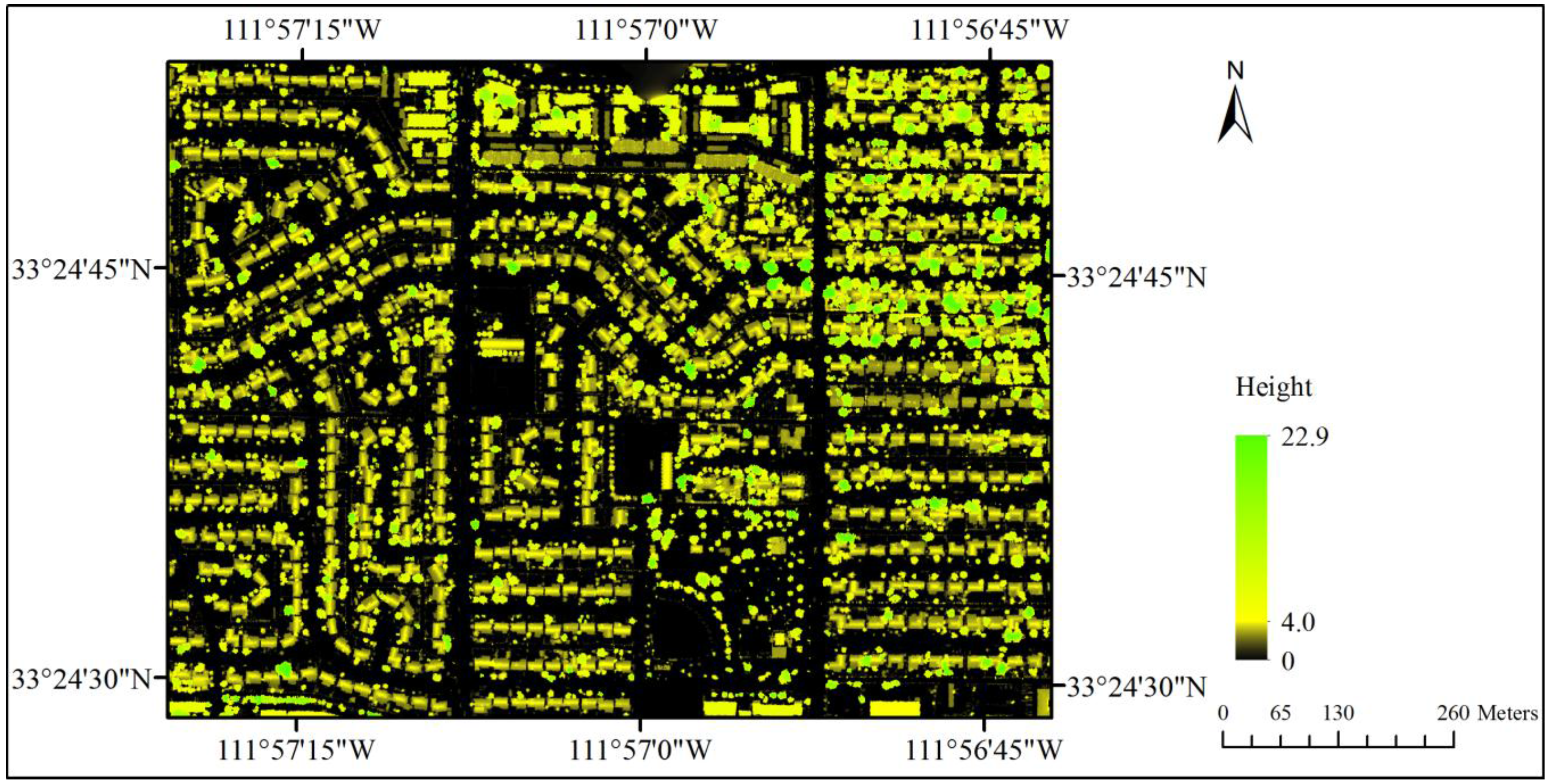
First and last vertical returns were derived from the LIDAR point clouds, with an average point space of 0.6 m. The bare earth model was constructed from ground points (last return) with all the anthropogenic features removed. The digital surface model represents all the ground features such as buildings and vegetation, and was created from non-ground points (first return) (Figure 7). The normalized height surface was obtained by subtracting the bare earth model from digital surface model.

Figure 7. Normalized height surface derived by airborne LIDAR point clouds.

Figure 7. Normalized height surface derived by airborne LIDAR point clouds.

3.1.2. QuickBird Image Classification

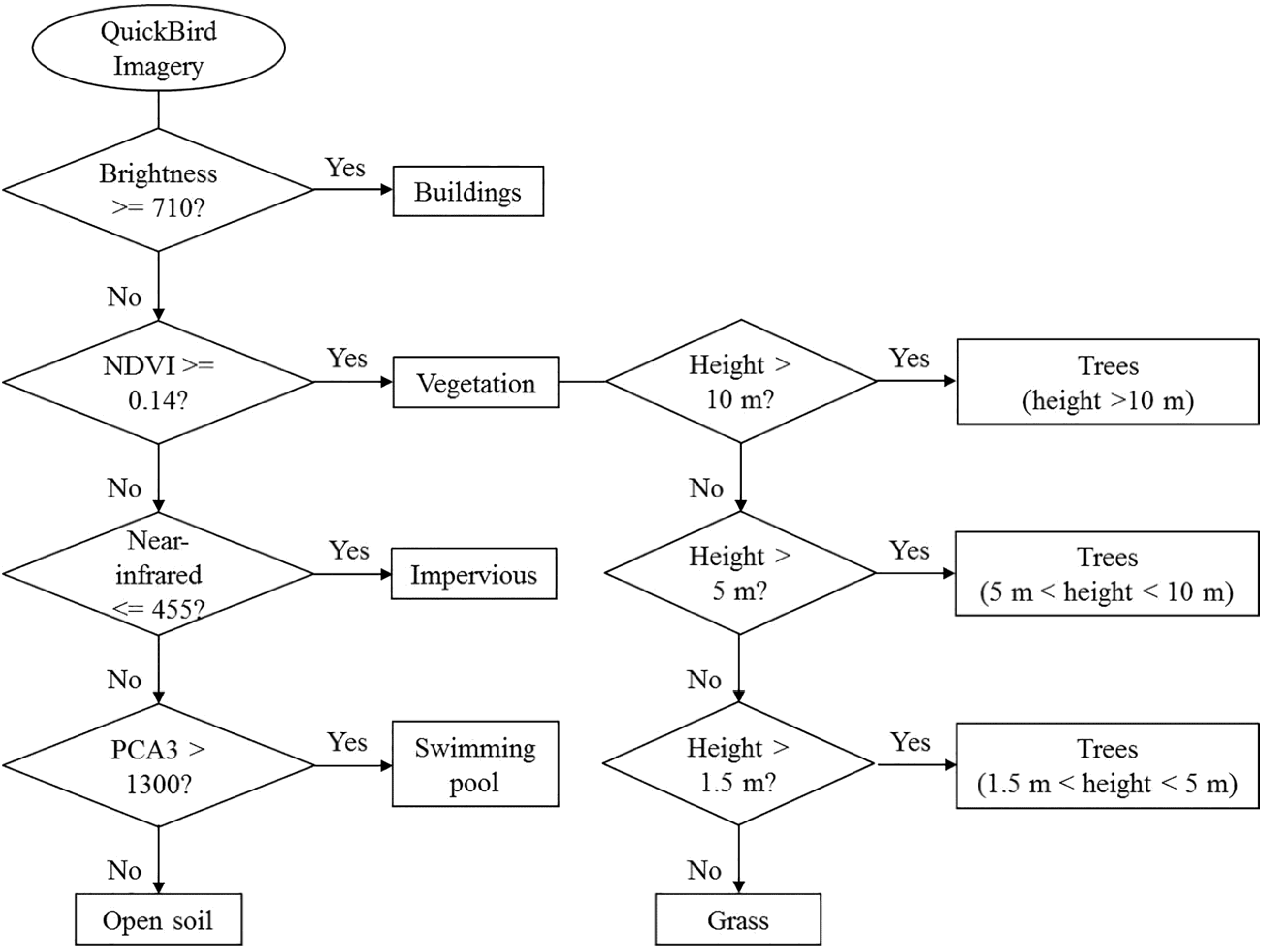
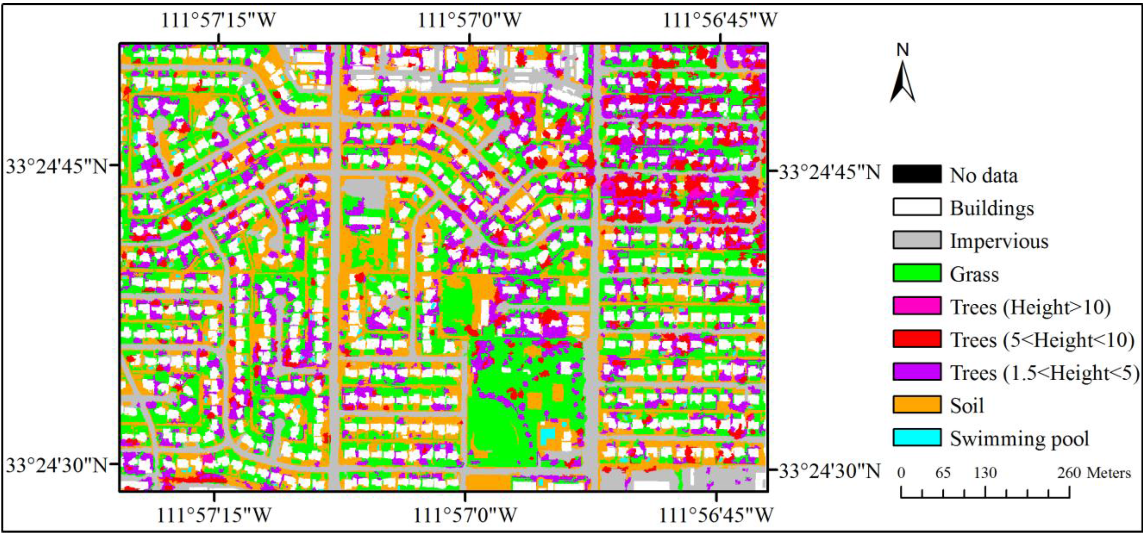
To preprocess QuickBird imagery for object-oriented classification, we first generated three principal component analysis (PCA) bands and layer-stacked with the original four bands, including blue, green, red, and near-infrared (NIR). The normalized height surface layer derived from the LIDAR was also incorporated into the dataset. Six major classes created using the object-oriented approach include: buildings, other impervious surfaces, grass, trees /shrubs, open soil, and swimming pool.

The object-oriented approach involves two major steps: image segmentation and image classification. The image was first hierarchical segmented into three levels with the scale level being 100, 50, and 10. The flow chart below describes the decision rule sets along with the classification hierarchy (Figure 8). Figure 9 shows the land use/cover map of the classification results. Table 1 describes the accuracy of the object-oriented classification approach, showing an overall accuracy of 90.4% and the kappa coefficient at 0.89.

Table 1. Classification accuracy of the object-oriented approach.

Classified	Reference							Producer’s Accuracy (%)	User’s Accuracy (%)
	Buildings	Open Soil	Grass	Impervious	Pools	Trees/Shrubs	Total
Buildings	73	2	1	3	0	1	80	83.91	91.25
Open soil	6	70	0	3	1	0	80	94.59	87.50
Grass	6	2	68	2	0	8	86	95.77	79.07
Impervious	1	0	0	87	0	0	88	83.65	98.86
Pools	1	0	0	1	48	0	50	97.96	96.00
Trees/shrubs	0	0	2	8	0	56	66	86.15	84.85
Total	87	74	71	104	49	65	450
Overall accuracy = 90.40%; Overall kappa statistics = 0.89

Table 1. Classification accuracy of the object-oriented approach.

Classified	Reference							Producer’s Accuracy (%)	User’s Accuracy (%)
	Buildings	Open Soil	Grass	Impervious	Pools	Trees/Shrubs	Total
Buildings	73	2	1	3	0	1	80	83.91	91.25
Open soil	6	70	0	3	1	0	80	94.59	87.50
Grass	6	2	68	2	0	8	86	95.77	79.07
Impervious	1	0	0	87	0	0	88	83.65	98.86
Pools	1	0	0	1	48	0	50	97.96	96.00
Trees/shrubs	0	0	2	8	0	56	66	86.15	84.85
Total	87	74	71	104	49	65	450
Overall accuracy = 90.40%; Overall kappa statistics = 0.89

Figure 8. Decision rules for object-oriented classification.

Figure 8. Decision rules for object-oriented classification.

Figure 9. Land use/land cover map from QuickBird imagery.

Figure 9. Land use/land cover map from QuickBird imagery.

3.1.3. Surrounding Trees and Exposed Rooftops Extraction

To accurately measure the relative building-tree geometry, trees were further categorized into three subclasses: tree height > 10 m, 5–10 m, and 1.5–5 m by using the normalized height surface. Land cover cells classified as trees with a height value > 10 meters were defined as tall trees. Similarly, cells classified as trees with height values between 5 meters and 10 meters were categorized as medium trees and < 5 meters were classified as small trees.

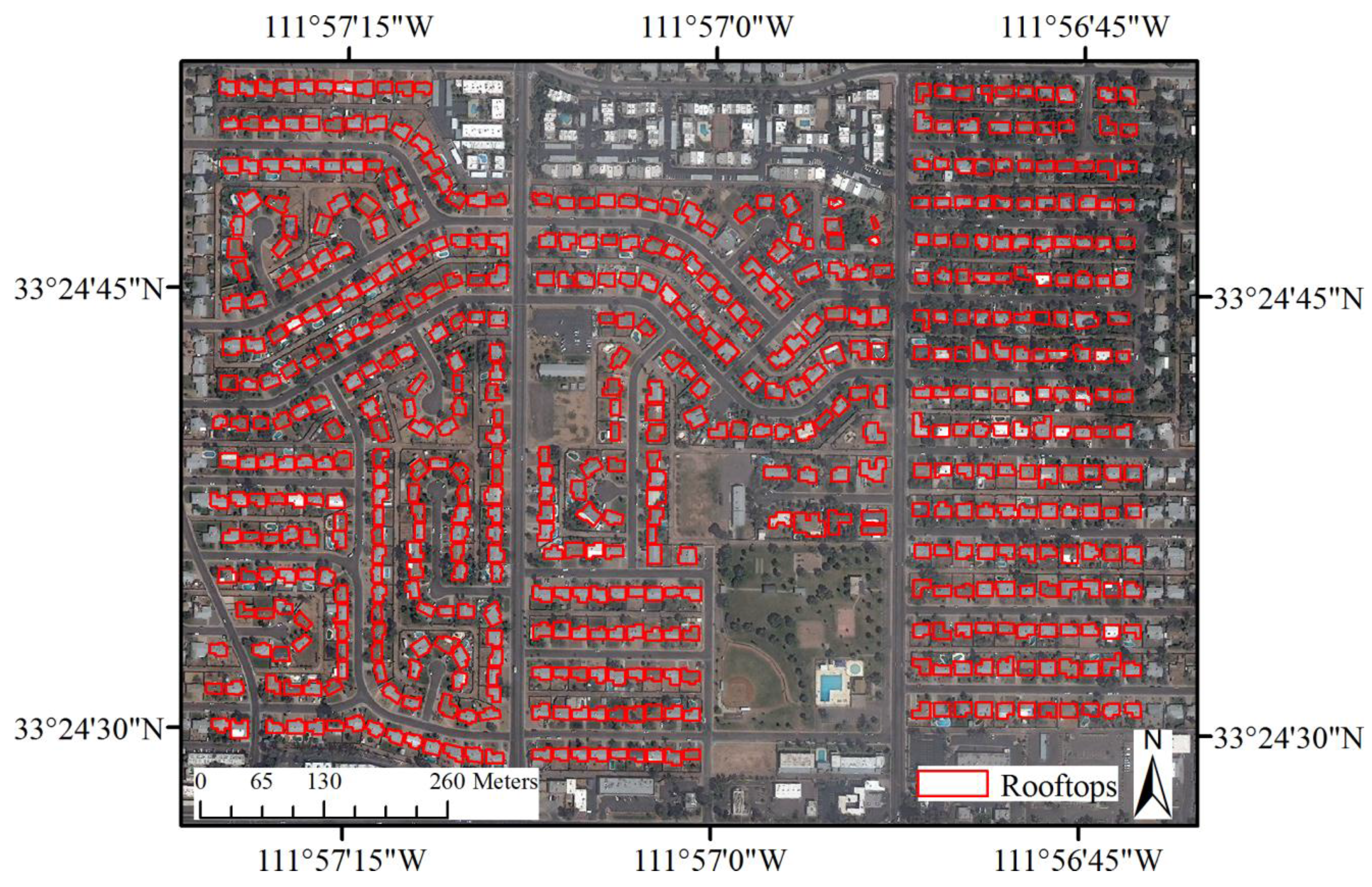
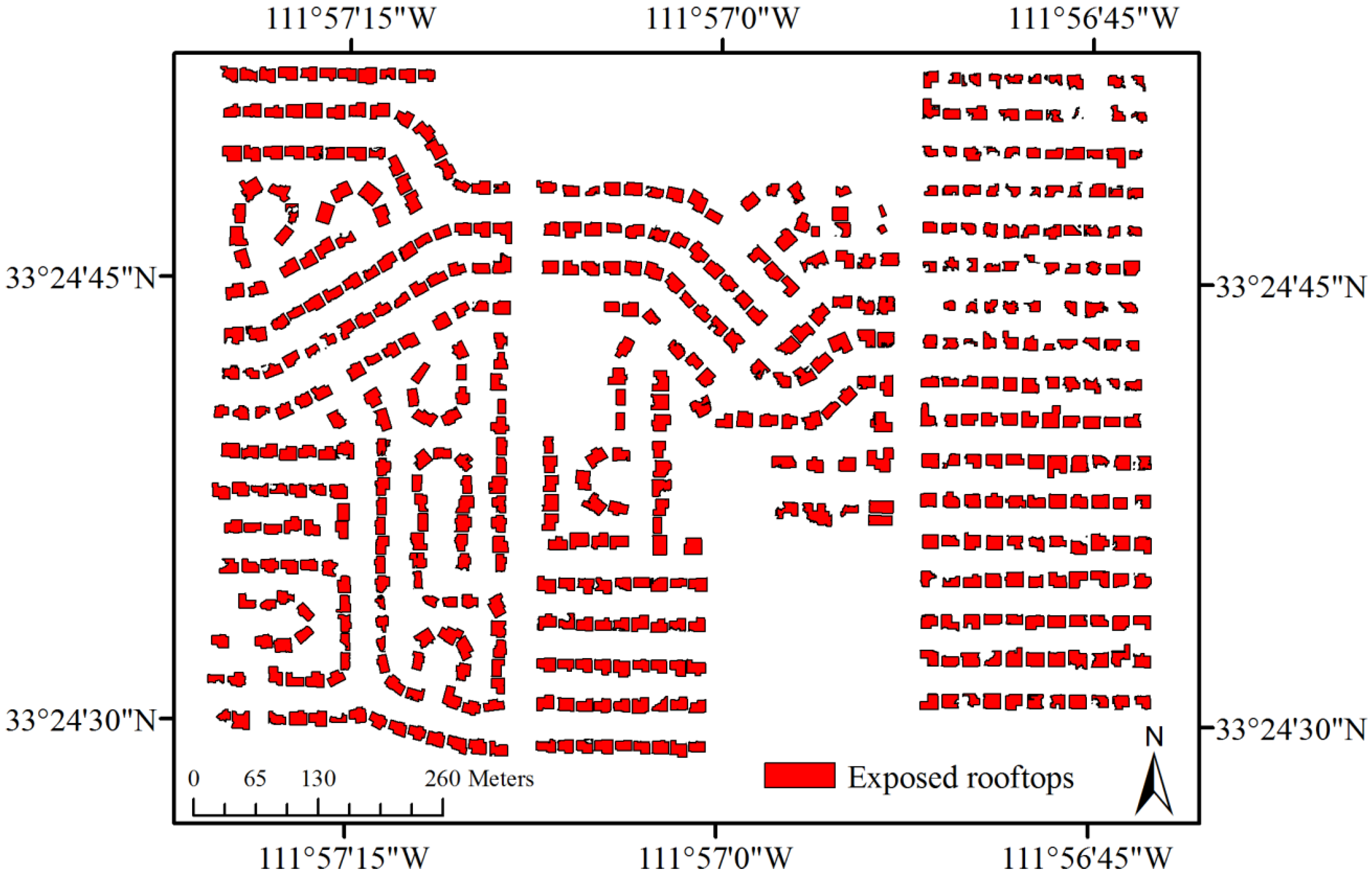
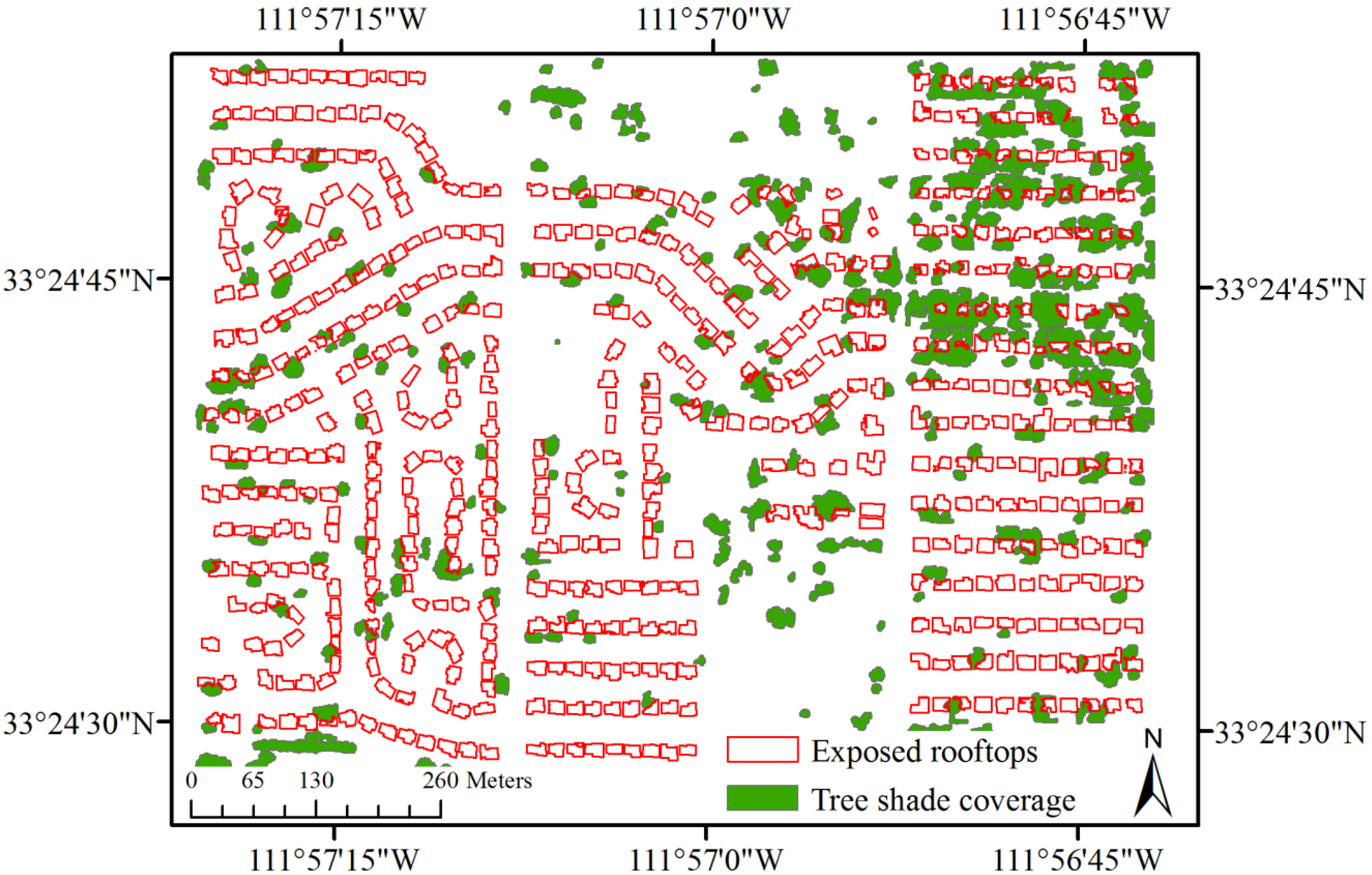
To obtain exposed rooftops for the subsequent analysis, tree canopies that were overhung on rooftops were eliminated. Rooftop footprints were erased by tree canopies based on the classification results from QuickBird imagery (Figure 10). Considering the effect of tree shade to the building rooftops, tall trees, and medium height trees (tree height > 5 meters) were utilized to estimate the tree shade range. According to the imagery acquisition time of MASTER imagery (11am–12pm, 12 July 2011), solar elevation angle was calculated based on the relative position of the sun and the earth. Shadow length was calculated as below.

$$L=\left(h_t-h_r\right)/\text{tan }\beta$$

(1)

$L$ is the shadow length, $h_t$ is the average height of the trees, $h_r$ is the average height of the rooftops and $\beta$ is the solar elevation angle. Through Equation (1), we used the average shadow length of 1.5 meters as our buffer distance. Then we applied a buffer analysis to our tree canopies layer for further analysis (Figure 11).

Figure 10. Exposed rooftops.

Figure 10. Exposed rooftops.

Figure 11. Tree shade.

Figure 11. Tree shade.

3.2. Rooftop Parameter Extraction

3.2.1. Configuration Parameters

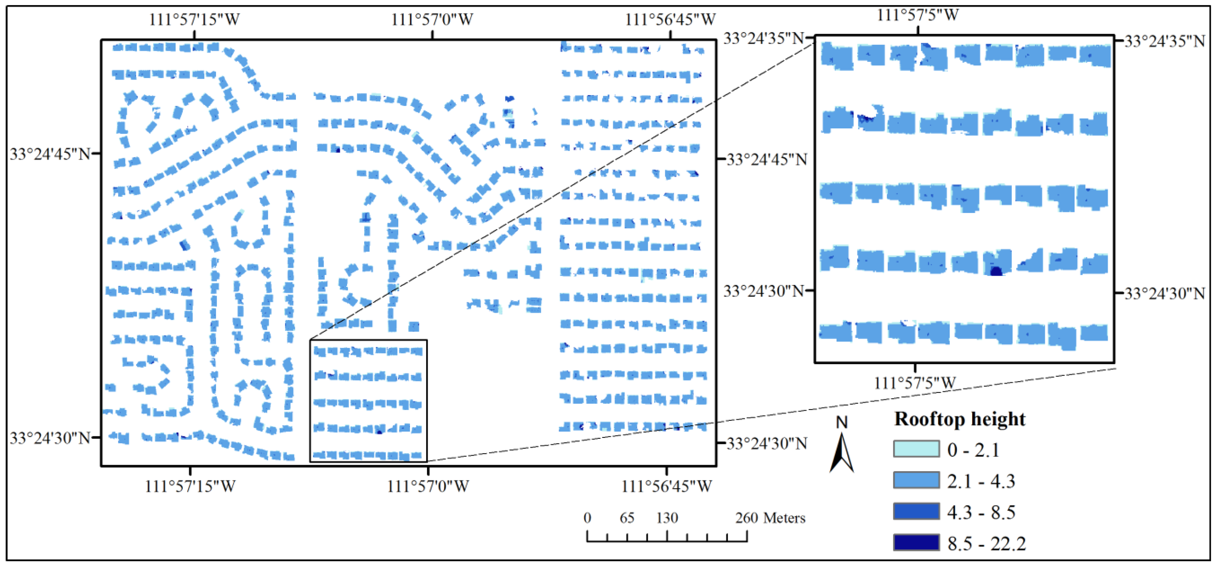
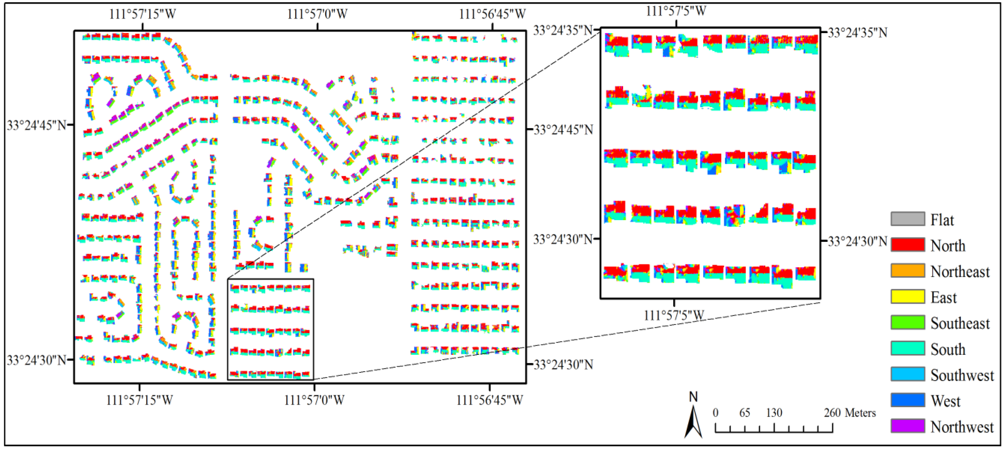
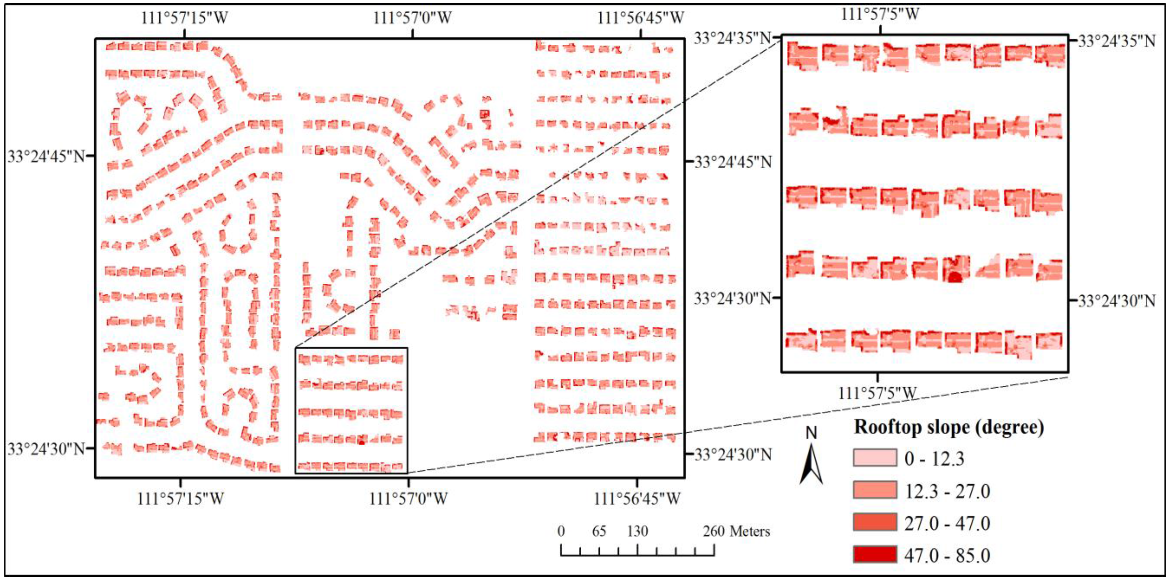
We used normalized height surface to calculate configuration parameters of rooftops. Rooftop height and rooftop area were easily derived by intersecting exposed rooftops and normalized height surface (Figure 12). We created slope and aspect layers through spatial analyst tools in a GIS environment (Figure 13 and Figure 14).

Figure 12. Rooftop height.

Figure 12. Rooftop height.

Figure 13. Rooftop slope.

Figure 13. Rooftop slope.

Figure 14. Rooftop aspect.

Figure 14. Rooftop aspect.

3.2.2. Reflectance Conversion and Albedo Estimation

Radiometric correction was conducted with the aid of QuickBird metadata and the radiance conversion algorithm [62]. The radiance conversion algorithm first transformed DN (digital number) to top-of-atmosphere spectral radiance, then to band-averaged spectral radiance. Based on spectral radiance at the sensor’s aperture, earth-sun distance, mean solar exoatmospheric irradiances and solar zenith angle from the image acquisition’s metadata, the blue, green, red, and NIR band-averaged spectral radiance were calibrated to top of atmosphere reflectance [63].

An image calibration conducted by Kaplan et al. [64] was applied to estimate the daytime high resolution land surface broadband albedo through QuickBird reflectance. The albedo can be calculated using the following equation derived from multiple linear regression:

$$\text{α}= -1.694b_1 +2.749b_2 +0.288b_4$$

(2)

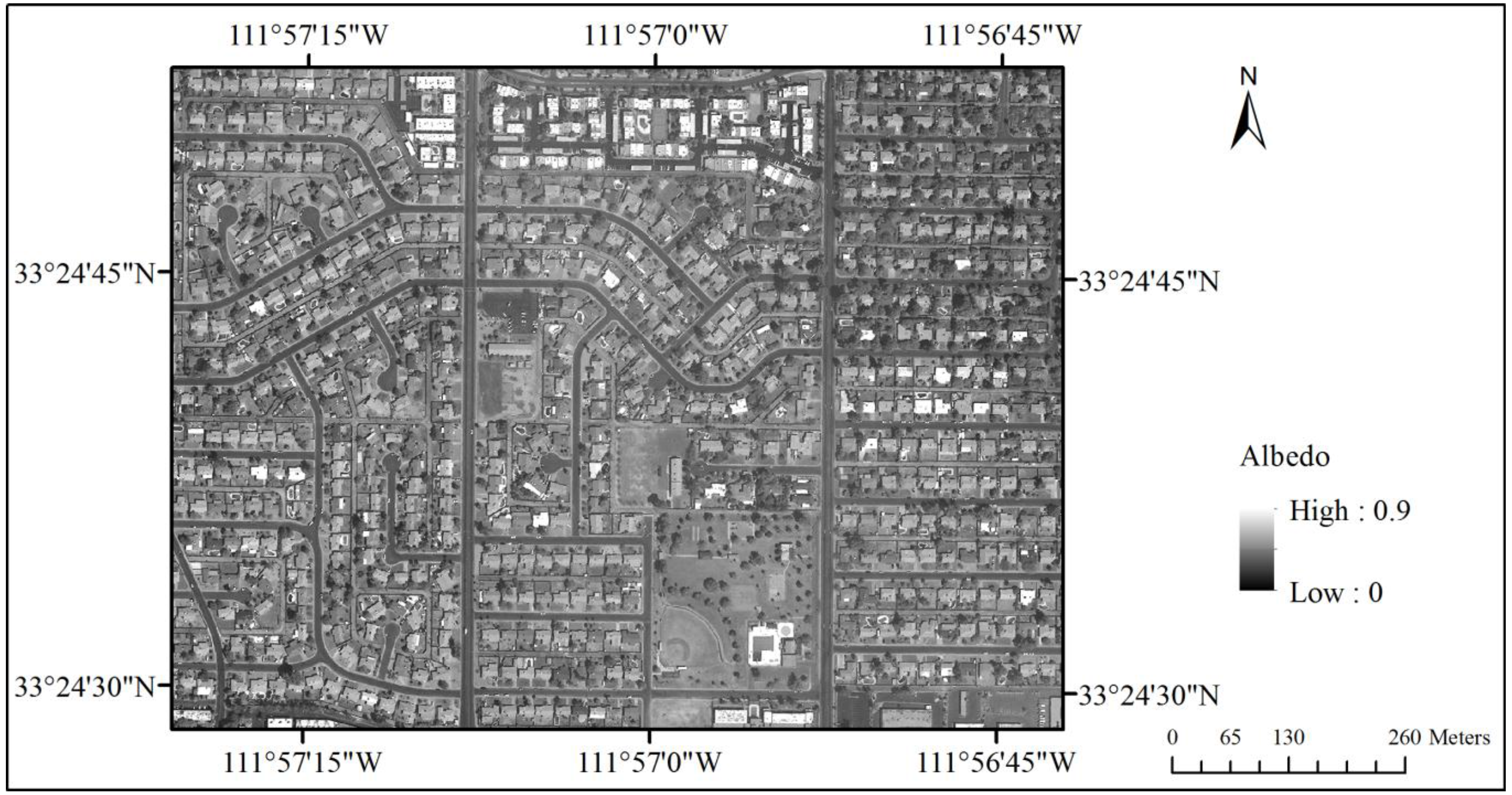
$\alpha$ is the estimated albedo from QuickBird imagery. $b_1,b_2,b_3$, and $b_4$ represent blue, green, red, and NIR reflectance, respectively. Because the red reflectance of QuickBird imagery was not statistically significant in the regression analysis [64], $b_3$ was not included in Equation (2). Figure 15 shows the rooftop albedo estimation results.

Figure 15. Albedo estimated from QuickBird imagery.

Figure 15. Albedo estimated from QuickBird imagery.

3.2.3. Surface Temperature Extraction

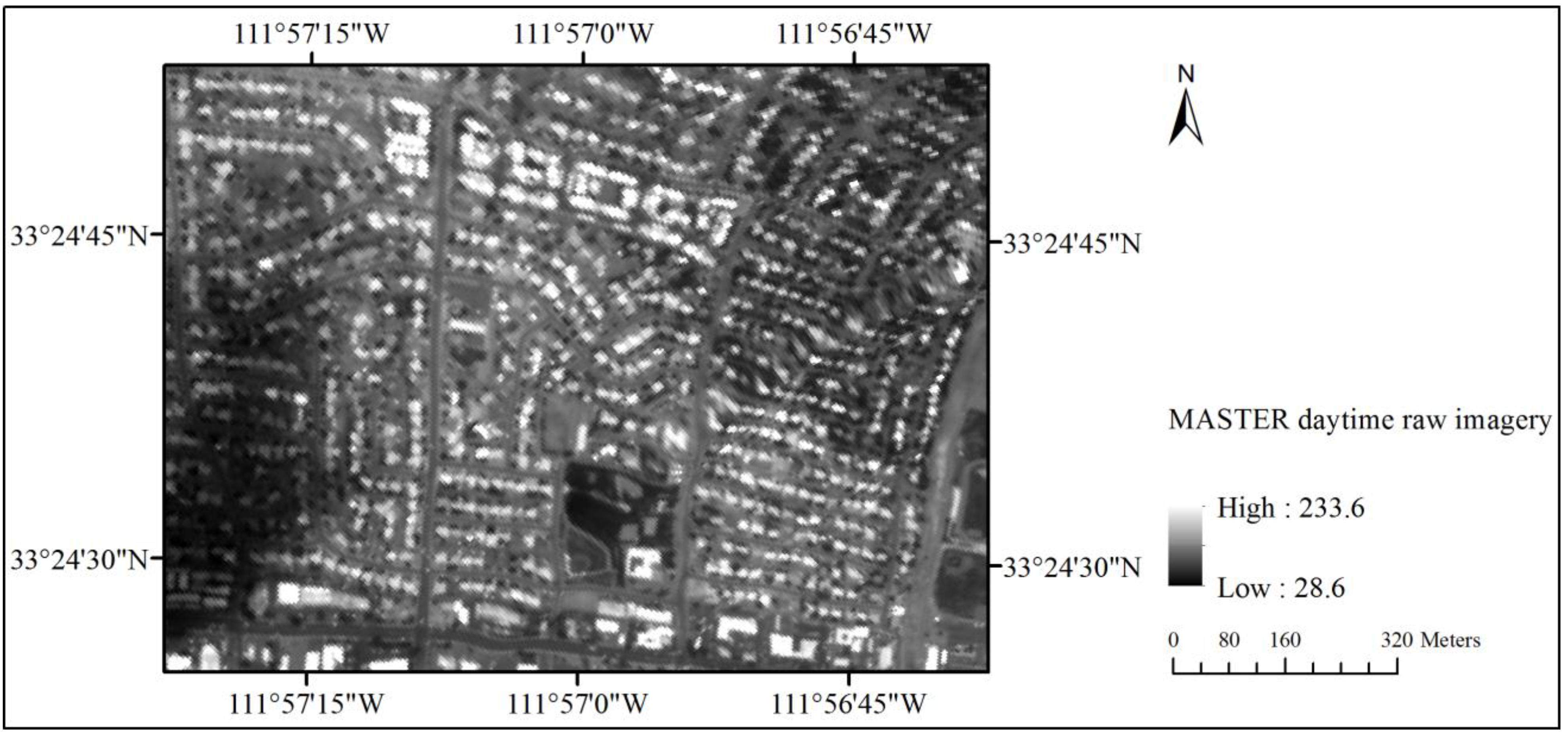
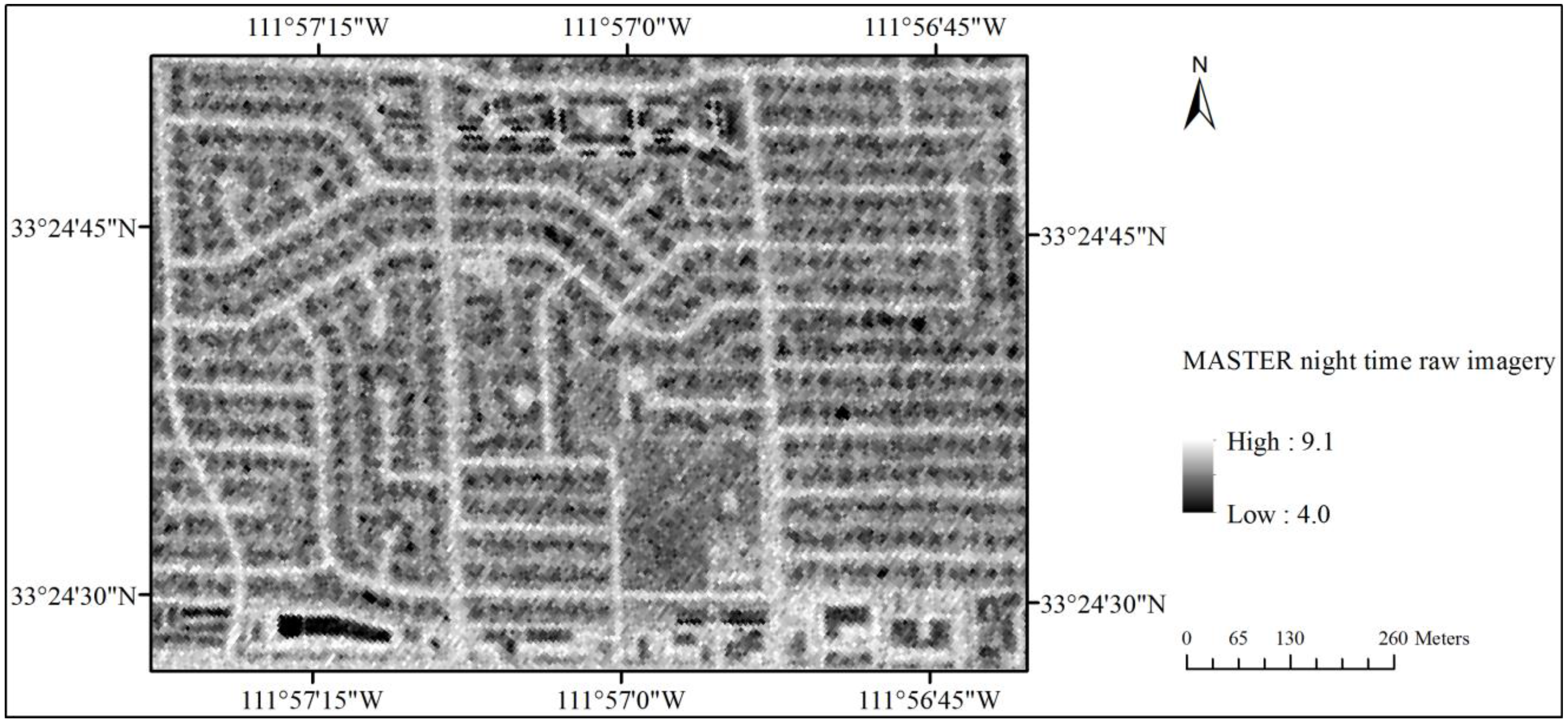
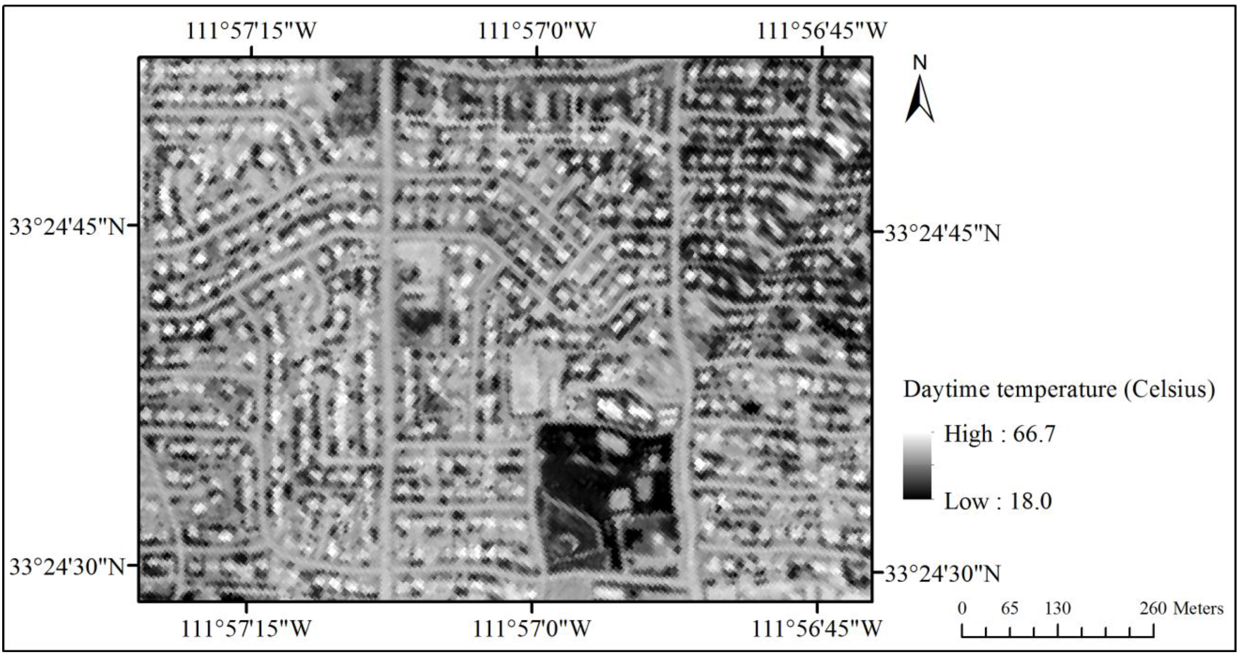
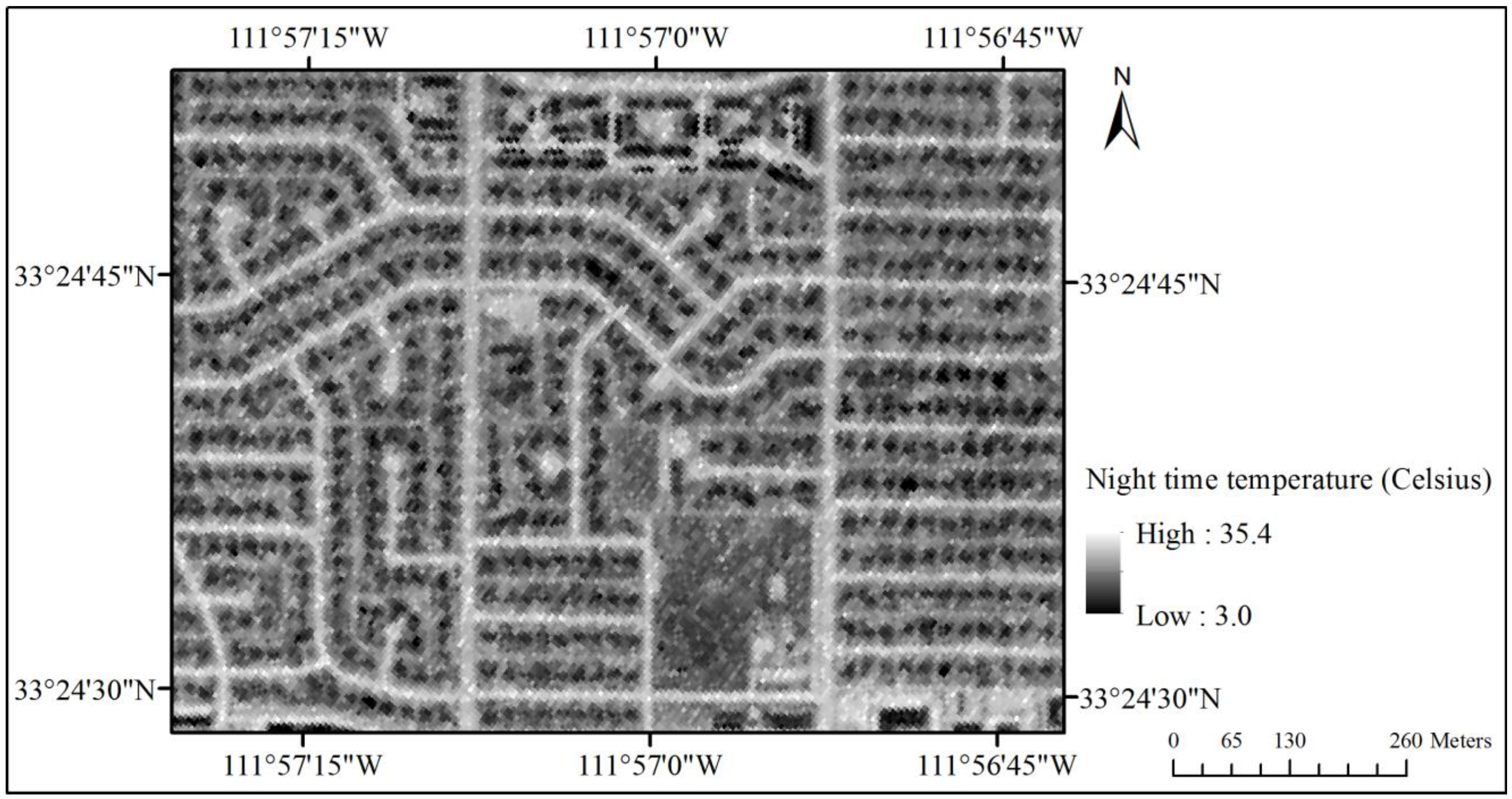
MASTER imagery provides fine-resolution thermal details (7 m) and serves as the thermal data source in our detailed rooftop temperature analysis. Atmospheric correction of the mid-infrared wavelength data was conducted using an in-scene atmospheric compensation technique, which was followed by separation of emissivity and surface temperature by an emissivity normalization approach [65,66,67,68]. Further, NAIP imagery was utilized to georeference because its similar spatial resolution with the MASTER imagery and both images were acquired close in time. We chose 80 ground control points from NAIP and daytime/night time MASTER imagery and used second order polynomials and nearest neighbor resampling to produce the best image warping results. The RMS error for daytime MASTER imagery was 0.41, for night time MASTER imagery was 0.26. The daytime and night time MASTER imagery were shown in Figure 16 and Figure 17.

Figure 16. Daytime temperature derived from MASTER imagery.

Figure 16. Daytime temperature derived from MASTER imagery.

Figure 17. Night time temperature derived from MASTER imagery.

Figure 17. Night time temperature derived from MASTER imagery.

3.3. Regression Analysis

To successfully employ regression analysis, image subset, registration, and layer stack is necessary. Table 2 shows the summary statistics for selected rooftop parameters. Because the daytime MASTER imagery has a large distortion area, only 383 rooftop samples were used in the daytime temperature analysis, compared to 567 samples for night time imagery.

Table 2. Statistics of the selected rooftop parameters.

	Daytime Analysis (383 Samples)	Night Time Analysis (567 Samples)
Area (m2)
Minimum	54.78	24.35
Maximum	454.78	454.77
Mean	208.44	197.69
Standard deviation	48.15	53.13
Height (m)
Minimum	2.42	2.27
Maximum	3.32	6.73
Mean	3.12	3.16
Standard deviation	0.29	0.37
Slope (degree)
Minimum	10.34	7.83
Maximum	36.20	36.72
Mean	21.01	20.98
Standard deviation	3.08	3.70
Southeast (%)
Minimum	5.17	0
Maximum	38.69	38.69
Mean	7.65	6.94
Standard deviation	7.34	6.34
South (%)
Minimum	0.48	0.48
Maximum	50.89	60.49
Mean	18.65	21.05
Standard deviation	13.03	12.34

Table 2. Statistics of the selected rooftop parameters.

	Daytime Analysis (383 Samples)	Night Time Analysis (567 Samples)
Area (m2)
Minimum	54.78	24.35
Maximum	454.78	454.77
Mean	208.44	197.69
Standard deviation	48.15	53.13
Height (m)
Minimum	2.42	2.27
Maximum	3.32	6.73
Mean	3.12	3.16
Standard deviation	0.29	0.37
Slope (degree)
Minimum	10.34	7.83
Maximum	36.20	36.72
Mean	21.01	20.98
Standard deviation	3.08	3.70
Southeast (%)
Minimum	5.17	0
Maximum	38.69	38.69
Mean	7.65	6.94
Standard deviation	7.34	6.34
South (%)
Minimum	0.48	0.48
Maximum	50.89	60.49
Mean	18.65	21.05
Standard deviation	13.03	12.34

To explore the relationships among rooftop surface temperature, rooftop configuration, and rooftop spectral property, ordinary least squares regression (OLS) was conducted. The dependent variable was the rooftop surface temperature derived from MASTER imagery on daytime or night time. The independent variables were rooftop configuration variables, which are slope, height, area, aspect, and rooftop spectral property, which is the surface reflectance/albedo. Rooftop aspect entered the regression model by a ratio of rooftop area (eight cardinal directions, north, south, east, west, northwest, northeast, southwest, and southeast). Stepwise regression method helped determine the best regression model to predict temperature. To evaluate outdoor landscaping effects, a dummy variable was created in regression analysis. If the rooftop intersected with the tree shade layer, we evaluated whether the outdoor landscaping influenced the rooftop surface temperature, and set the dummy variable to 1, otherwise it was set to 0. Detailed results and discussions from the regression analysis are reported in the next two sections.

4. Results

Table 3 reports descriptive statistics of selected dependent and independent variables. The standard deviation of daytime temperature is 2.63 Celsius degrees, and 1.01 Celsius degrees for night time temperature. Similarly, blue, green, red, and NIR reflectance and estimated albedo have small standard deviations. These low standard deviation values illustrate the similarity of rooftops in this residential neighborhood. Because we use a dummy variable to represent the shading effects of nearby trees, the minimum and maximum of this variable are 0 and 1. 31% of the rooftops have tree shade effects for daytime analysis.

Table 3. Descriptive statistics of the selected dependent and independent variables.

	Daytime Analysis (383 Samples)	Night Time Analysis (567 Samples)
Temperature (Celsius degree)
Minimum	43.99	13.70
Maximum	59.94	24.29
Mean	53.89	19.85
Standard deviation	2.63	1.01
Blue reflectance
Minimum	0.13	0.13
Maximum	0.32	0.35
Mean	0.19	0.20
Standard deviation	0.03	0.03
Green reflectance
Minimum	0.12	0.12
Maximum	0.33	0.36
Mean	0.19	0.19
Standard deviation	0.03	0.03
Red reflectance
Minimum	0.13	0.12
Maximum	0.36	0.40
Mean	0.21	0.21
Standard deviation	0.03	0.04
NIR reflectance
Minimum	0.17	0.17
Maximum	0.44	0.46
Mean	0.25	0.25
Standard deviation	0.03	0.04
Estimated albedo
Minimum	0.16	N/A
Maximum	0.49	N/A
Mean	0.27	N/A
Standard deviation	0.04	N/A
Nearby tree shade (a dummy variable)
Minimum	0	N/A
Maximum	1	N/A
Mean	0.31	N/A
Standard deviation	0.46	N/A

Table 3. Descriptive statistics of the selected dependent and independent variables.

	Daytime Analysis (383 Samples)	Night Time Analysis (567 Samples)
Temperature (Celsius degree)
Minimum	43.99	13.70
Maximum	59.94	24.29
Mean	53.89	19.85
Standard deviation	2.63	1.01
Blue reflectance
Minimum	0.13	0.13
Maximum	0.32	0.35
Mean	0.19	0.20
Standard deviation	0.03	0.03
Green reflectance
Minimum	0.12	0.12
Maximum	0.33	0.36
Mean	0.19	0.19
Standard deviation	0.03	0.03
Red reflectance
Minimum	0.13	0.12
Maximum	0.36	0.40
Mean	0.21	0.21
Standard deviation	0.03	0.04
NIR reflectance
Minimum	0.17	0.17
Maximum	0.44	0.46
Mean	0.25	0.25
Standard deviation	0.03	0.04
Estimated albedo
Minimum	0.16	N/A
Maximum	0.49	N/A
Mean	0.27	N/A
Standard deviation	0.04	N/A
Nearby tree shade (a dummy variable)
Minimum	0	N/A
Maximum	1	N/A
Mean	0.31	N/A
Standard deviation	0.46	N/A

Pearson’s correlation among four reflectance bands from QuickBird and estimated albedo is shown in Table 4. With all correlations > 0.89, there is a high correlation among all variables with reflectance and estimated albedo. Thus, either albedo or reflectance was entered into a regression model at any one time. Table 5 and Table 6 report on different regression models based on different spectral bands. Because each model has the same parameters, we can compare these results and decide which spectral bands contribute most to understanding rooftop surface temperature. From the R-square adjusted value, NIR reflectance and albedo represent good spectral parameters to explain variations in rooftop surface temperature. Detailed regression analysis results by using NIR reflectance band and estimated albedo layer as spectral information will be discussed next.

Table 4. Pearson correlation between reflectance and albedo.

	Blue	Green	Red	NIR
Green	0.991 *
Red	0.939 *	0.974 *
NIR	0.893 *	0.929 *	0.950 *
Albedo	0.940 *	0.977 *	0.991 *	0.970 *
All the p-value = 0.000

* represents high correlation between two variables.

Table 4. Pearson correlation between reflectance and albedo.

	Blue	Green	Red	NIR
Green	0.991 *
Red	0.939 *	0.974 *
NIR	0.893 *	0.929 *	0.950 *
Albedo	0.940 *	0.977 *	0.991 *	0.970 *
All the p-value = 0.000

* represents high correlation between two variables.

Table 5. Regression comparison (daytime).

	Blue	Green	Red	NIR	Albedo (estimated)
R2 (%)	27.99	28.69	27.83	31.38	29.19
R2 (adj) (%)	26.84	27.55	26.68	30.28	28.06

Every model has same parameters. All the p-value < 0.05.

Table 5. Regression comparison (daytime).

	Blue	Green	Red	NIR	Albedo (estimated)
R2 (%)	27.99	28.69	27.83	31.38	29.19
R2 (adj) (%)	26.84	27.55	26.68	30.28	28.06

Every model has same parameters. All the p-value < 0.05.

Table 6. Regression comparison (night time).

	Blue	Green	Red	NIR
R2 (%)	16.98	16.97	16.86	17.74
R2 (adj) (%)	16.69	16.68	16.56	17.45

Every model has same parameters. All the p-value < 0.05.

Table 6. Regression comparison (night time).

	Blue	Green	Red	NIR
R2 (%)	16.98	16.97	16.86	17.74
R2 (adj) (%)	16.69	16.68	16.56	17.45

Every model has same parameters. All the p-value < 0.05.

4.1. Regression Analysis Results for the Daytime Rooftop Temperature

Table 7 describes the regression analysis results among daytime rooftop surface temperature, rooftop configuration parameters, NIR reflectance, and influence of surrounding trees. Variable selection was estimated by stepwise regression methods [69]. In Equation (3), $T_d$ is the average daytime temperature of each rooftop, $A$ is the rooftop surface area, $SE$ and $S$ represent the ratio of rooftop area facing southeast and south, $s$ is the average slope of each rooftop, $b_4$ is the NIR reflectance from QuickBird imagery and $N_t$ is the dummy variables for nearby landscaping. By using all of these variables, we successfully explain 30.28% of the daytime rooftop temperature.

Regression equation:

$$T_d= 64.33+0.00572A +7.74SE +4.507S-0.1080s-43.23 b_4-0.637 N_t$$

(3)

Table 7. Daytime regression analysis results by NIR reflectance.

Model Summary
S		R2		R2 (adj)		R2 (pred)
2.20081		31.38%		30.28%		28.31%
Coefficients
Variable	Coefficient		SE Coef		t-statistic		p-value
Constant	64.33		1.370		46.87		0.000
Area	0.00572		0.00244		2.34		0.020
Southeast	7.74		1.650		4.68		0.000
South	4.507		0.918		4.91		0.000
Slope	−0.1080		0.0378		−2.86		0.004
NIR	−43.23		3.570		−12.11		0.000
Nearby tree shade	−0.637		0.250		−2.54		0.011
95% statistically significant.

Table 7. Daytime regression analysis results by NIR reflectance.

Model Summary
S		R2		R2 (adj)		R2 (pred)
2.20081		31.38%		30.28%		28.31%
Coefficients
Variable	Coefficient		SE Coef		t-statistic		p-value
Constant	64.33		1.370		46.87		0.000
Area	0.00572		0.00244		2.34		0.020
Southeast	7.74		1.650		4.68		0.000
South	4.507		0.918		4.91		0.000
Slope	−0.1080		0.0378		−2.86		0.004
NIR	−43.23		3.570		−12.11		0.000
Nearby tree shade	−0.637		0.250		−2.54		0.011
95% statistically significant.

Table 8 is the regression analysis results among from daytime rooftop surface temperature, rooftop configuration parameters, estimated albedo layer, and influence of surrounding trees. In Equation (4), $\alpha$ is the estimated albedo based on Kaplan et al. [64]. Other parameters are the same as Equation (3). By using albedo, we explain 28.06% of the daytime rooftop temperature.

Regression equation:

$$T_d= 62.73+0.00651A +6.96SE +4.223S-0.1070s-33.00 \alpha -0.840 N_t$$

(4)

Table 8. Daytime regression analysis results by albedo.

Model Summary
S		R2		R2 (adj)		R2 (pred)
2.23553		29.19%		28.06%		26.03%
Coefficients
Variable	Coefficient		SE Coef		t-statistic		p-value
Constant	62.73		1.330		47.10		0.000
Area	0.00651		0.00250		2.61		0.009
Southeast	6.96		1.670		4.17		0.000
South	4.223		0.930		4.54		0.000
Slope	−0.1070		0.0384		−2.79		0.006
Albedo	−33.00		2.890		−11.43		0.000
Nearby tree shade	−0.840		0.254		−3.31		0.001
95% statistically significant.

Table 8. Daytime regression analysis results by albedo.

Model Summary
S		R2		R2 (adj)		R2 (pred)
2.23553		29.19%		28.06%		26.03%
Coefficients
Variable	Coefficient		SE Coef		t-statistic		p-value
Constant	62.73		1.330		47.10		0.000
Area	0.00651		0.00250		2.61		0.009
Southeast	6.96		1.670		4.17		0.000
South	4.223		0.930		4.54		0.000
Slope	−0.1070		0.0384		−2.79		0.006
Albedo	−33.00		2.890		−11.43		0.000
Nearby tree shade	−0.840		0.254		−3.31		0.001
95% statistically significant.

Table 7 and Table 8 report the detailed regression analysis results from the daytime rooftop surface temperature, rooftop configuration parameters, rooftop spectral property, and surrounding trees’ effects. In daytime temperature analysis, the NIR reflectance from QuickBird imagery and estimated albedo negatively and strongly contributes to the daytime rooftop surface temperature, which means high reflectance/albedo of rooftops result in low daytime temperature. Southeastern and southern parts of rooftops positively contribute to the daytime rooftop surface temperature. For rooftop configuration parameters, slope negatively contributes to the rooftop surface temperature but area positively contributes to the rooftop surface temperature. Furthermore, their influence is subtle. Surrounding trees decrease daytime rooftop temperature, which supports reasoning that outdoor landscaping is important for cooling residential living environment.

4.2. Regression Analysis Results for the Night Time Temperature

Table 9 reports the regression analysis results among night time rooftop surface temperature, rooftop configuration parameters, NIR reflectance and influence of surrounding trees. In Equation (5), $T_n$ is the night time temperature of rooftops, $s$ is the average slope of each rooftop and $b_4$ is the NIR reflectance from QuickBird imagery. From the regression analysis results, only slope and NIR reflectance are statistically significant to explain night time temperature. High reflectance results in low night time temperature. We explain 17.45% of the night time rooftop temperature by these two parameters.

Regression equation:

$$T_n= 18.792+0.0960s-3.81 b_4$$

(5)

Table 9. Night time regression analysis results by NIR reflectance.

Model Summary
S		R2		R2 (adj)		R2 (pred)
0.918805		17.74%		17.45%		16.68%
Coefficients
Variable	Coefficient		SE Coef		t-statistic		p-value
Constant	18.792		0.396		47.42		0.000
Slope	0.0960		0.0110		8.76		0.000
NIR	−3.81		1.030		−3.70		0.000
95% statistically significant.

Table 9. Night time regression analysis results by NIR reflectance.

Model Summary
S		R2		R2 (adj)		R2 (pred)
0.918805		17.74%		17.45%		16.68%
Coefficients
Variable	Coefficient		SE Coef		t-statistic		p-value
Constant	18.792		0.396		47.42		0.000
Slope	0.0960		0.0110		8.76		0.000
NIR	−3.81		1.030		−3.70		0.000
95% statistically significant.

Table 9 describes the detailed regression analysis results for the night time rooftop surface temperature. High rooftop NIR reflectance results in a low rooftop temperature at night, which is similar with the daytime results. Compared to the daytime rooftop temperature, spectral parameters contribute less to night time rooftop temperature. Similar to daytime results, rooftop slope still has some influence on the night time rooftop surface temperature.

5. Discussion

The UHI effect is typically stronger as a night time phenomenon where impervious surfaces associated with urban structures retain heat from daytime insolation [36]. We therefore analyzed the factors that influence both daytime and night time rooftop surface temperatures to understand this relationship at a structural level. We found that that rooftop characteristics can explain over 30% of the variation in daytime rooftop surface temperatures and slightly more than 17% of the night time temperatures. The stronger daytime adjusted R² with six significant explanatory variables suggest that direct solar insolation rather than heat retention of rooftop materials explained temperature variations. Without incoming solar radiation, the independent variables associated with roof aspect and the outdoor landscaping no longer contribute to rooftop surface temperatures. These results suggest that for energy efficiency during the daytime, appropriately placed tall trees can reduce rooftop temperatures. The night time UHI temperatures commonly reported in UHI studies remain associated with impervious surfaces of pavement and other hard surfaces rather than rooftop temperature variations.

The conventional wisdom that suggests warmer surfaces are on southern exposures in the northern hemisphere is confirmed in this study. The three significant variables that were positively correlated with increasing daytime rooftop temperatures are southeast and south facing roof surfaces and rooftop area. The southeast and south aspect were positively correlated with warmer rooftop temperatures because of the direct incoming solar radiation. The southwest aspect was not significant (as conventional wisdom might suggest) because the imagery acquisition time of the daytime MASTER imagery was 11 am–12 pm, 12 July. Larger roof areas were warmer because the larger surface area would provide more homogeneity and therefore continuity of insolation, much like the cluster effect of land covers reported at smaller scales [37]. These results suggest that building designs with smaller rooftop areas and buildings placed on lots to minimize southern roof exposure could result in lower rooftop surface temperatures.

Our study shows that in addition to reducing area and southern exposures, rooftop materials that reflect higher NIR reflectance and nearby trees could reduce daytime rooftop temperatures. Rooftop materials that have higher reflectance and minimize heat retention are an obvious design choice. Recognizing though that optimal design of buildings and building placement may not always be possible, our study shows that nearby trees can also aid in reducing daytime rooftop surface temperatures. Tree canopies coverage within 1.5 m of the structure can reduce rooftop surface temperatures between 0.64 °C and 0.84 °C. This finding is consistent with earlier UHI research that shows that the pattern of nearby vegetation contributes to lower UHI temperatures [17,18,20].

While we have strong determinants of daytime rooftop surface temperature, the only two independent variables in our models that explained night time rooftop temperature were NIR and slope. Variables associated with roof aspect and nearby vegetation did not contribute to the model. Like the daytime model, the higher NIR resulted in lower rooftop temperatures; supporting the idea that surface materials are an important consideration in reducing rooftop temperatures both during the day and at night. Unlike the daytime model, however, steeper roof slope in the night time model was associated with higher surface temperatures. While steeper sloped roofs are often a design consideration for dispersing rain and snow from building structures, there is little support here that suggests these design parameters may help in temperature relief as well.

Other parameters that likely influence rooftop temperature that we did not capture include indoor air conditioning, presence solar panels, age of rooftop, and materials and colors of rooftops. These parameters were not accessible through remotely sensed data sources, which was the focus of this study. Future research should consider an expanded study area and different geographical locations to capture more variation in rooftop materials and have more rooftop samples to derive the statistical results. A more detailed study could include ancillary features on the roof that potentially influence temperature such as the exhaust from air conditioning units and the role of solar panels. In addition to the rooftop parameters, the acquisition time of remote sensing imagery (solar angles) and existing errors (MASTER daytime imagery distortion) would potentially influence the albedo estimation process and regression analysis results. Future research will focus on obtaining other related parameters by fieldwork or survey to quantify UHI effect (near-surface temperature), optimizing outdoor landscaping design, and providing sustainable approaches to ameliorate UHI effectively.

6. Conclusions

This research explores the interrelationships between rooftop surface temperature, rooftop geophysical properties, rooftop configuration, and outdoor landscaping in an urban residential environment. High-resolution thermal imagery (MODIS/ASTER airborne simulator) enables detailed analysis of urban thermal characteristics at a neighborhood level. Airborne LIDAR point clouds make it possible to obtain rooftop configuration parameters such as rooftop aspect and slope, and also help us extract tree height information when integrated with the land cover classification map generated from very high resolution multispectral imagery. The results of the regression analysis explained around 30% of the daytime rooftop temperature and 17% of the night time rooftop temperature. Rooftop spectral properties were the major factors in influencing rooftop surface temperatures. At the same time, the sun’s position and surrounding landscaping (trees) influenced the temperature as well.

The research provides a method to understand the impact of urban landscaping and helps design the sustainable rooftops in an urban residential environment. From this research, we continue to illustrate that rooftop design choices will impact the urban heat island effect in the urban residential environment. The high-albedo rooftop materials will contribute significant cooling effects to single family households. Trees can ameliorate the UHI effects when they are planted on the south side of the households to block the direct sunlight on rooftops. All of these help residents save their energy usage for cooling technologies like air-conditioning, create a healthier living environment, and reduce urban heat island effects. This research connects the remote sensing technologies with the individual building structures. This new attempt not only provides a new approach to analyze urban heat island at a neighborhood level, but also offers a different method to study the relationships among buildings, energy, and urban environment.