Article

Remote Sensing Based Two-Stage Sampling for Accuracy Assessment and Area Estimation of Land Cover Changes

Remote Sensing and Geoinformation, Institute for Information and Communication Technologies, Joanneum Research, Steyrergasse 17, Graz A-8010, Austria
*
Author to whom correspondence should be addressed.
Remote Sens. 2015, 7(9), 11992-12008; https://doi.org/10.3390/rs70911992
Submission received: 20 May 2015 / Revised: 10 September 2015 / Accepted: 10 September 2015 / Published: 18 September 2015

Abstract

:
Land cover change processes are accelerating at the regional to global level. The remote sensing community has developed reliable and robust methods for wall-to-wall mapping of land cover changes; however, land cover changes often occur at rates below the mapping errors. In the current publication, we propose a cost-effective approach to complement wall-to-wall land cover change maps with a sampling approach, which is used for accuracy assessment and accurate estimation of areas undergoing land cover changes, including provision of confidence intervals. We propose a two-stage sampling approach in order to keep accuracy, efficiency, and effort of the estimations in balance. Stratification is applied in both stages in order to gain control over the sample size allocated to rare land cover change classes on the one hand and the cost constraints for very high resolution reference imagery on the other. Bootstrapping is used to complement the accuracy measures and the area estimates with confidence intervals. The area estimates and verification estimations rely on a high quality visual interpretation of the sampling units based on time series of satellite imagery. To demonstrate the cost-effective operational applicability of the approach we applied it for assessment of deforestation in an area characterized by frequent cloud cover and very low change rate in the Republic of Congo, which makes accurate deforestation monitoring particularly challenging.

Graphical Abstract

1. Introduction

Land cover change processes are accelerating from regional to global levels. Assessment of change processes is therefore urgently required in order to provide accurate and up-to-date information on past and current developments. The remote sensing community has developed increasingly reliable, consistent, and robust approaches for wall-to-wall mapping of land cover changes. Overall accuracy of the wall-to-wall maps is often in the range of 80% to 95%, depending on the source data, the change processes to be monitored, the biogeographic region, and the monitoring approach applied. Good overviews on methods for wall-to-wall land cover change monitoring are provided by [1,2].
A main requirement for operational applications, e.g., in the frame of international reporting for REDD (The United Nations Collaborative Programme on Reducing Emissions from Deforestation and Forest Degradation in Developing Countries), is that the wall-to-wall land cover change maps are complemented with accurate estimates of the area undergoing land cover changes [3].
The simplest approach to area estimation is to derive the area of land changes directly from the land cover change map. However, the errors of omission (error of excluding an area from a category to which it truly belongs, i.e., area underestimation) and errors of commission (error of including an area in a category to which it does not truly belong, i.e., area overestimation) are, in general, not equal. Such bias (systematic over- or under-estimation) shows up in the course of the accuracy assessment [4]. Adjusting area estimates on the basis of a rigorous accuracy assessment therefore represents an improvement over simply reporting the areas of classes as indicated on the map. The stratified estimator for area estimation based on error matrices was first introduced by [5]. Various approaches for area estimation have already been published for simple random, systematic, or stratified random sampling. A good overview of the general requirements for estimating area and assessing accuracy of land changes is given in [4,6]. They conclude that reporting only accuracy measures such as the overall accuracy and kappa coefficient is insufficient to fully address area estimation and uncertainty information needs.
A main requirement for operational applications such as REDD reporting is that confidence intervals are provided for the accuracy measures and area estimates. Methods for constructing confidence intervals for area estimates using error matrix information have been described, e.g., by [4,7], for popular sampling designs such as stratified random and simple random sampling. When reference data for two dates for different locations are used to estimate change for maps derived from post-classification, the methods described by [6,8,9] can be used for stratified random sampling designs. In [8,9], a model-assisted estimator with information from an error matrix is applied to compensate for bias as the result of classification errors and to estimate variances.
A variety of probability sampling designs can be used for accuracy assessment, area estimation, and derivation of confidence intervals. The decision in choosing a sampling design relates to trade-offs among different designs in terms of advantages to meet the specified requirements. A detailed review of sampling design options and how these designs fulfill different objectives and criteria is given in [10].
In the current publication, we propose an approach which specifically targets cost-effective application for large-area operational monitoring. The focus is on the sampling approach, which is applicable regardless of the procedure used to create the wall-to-wall land cover change map. The approach is exemplarily demonstrated for the assessment of deforestation in tropical forests in the Republic of Congo.

2. Methods

2.1. Overview and General Workflow

The monitoring approach is based on wall-to-wall land cover change mapping, which is complemented with a sampling approach for accuracy assessment, area estimation of land changes, and provision of confidence intervals. A two-stage sampling design is applied in order to keep accuracy, efficiency, and effort of the estimates in balance, while also taking limited availability of reference data such as cloud cover into account. In the first stage, area frames of a size of, for instance, 5 km by 5 km are selected as primary sampling units (PSUs). In the second stage, a set of pixels (secondary sampling units or SSUs) are sampled per PSU. Stratification is applied in both stages in order to gain control over the sample size allocated to rare land cover change classes on the one hand and cost constraints for acquisition and processing of reference imagery on the other. The general workflow of the approach is shown in Figure 1.
Figure 1. General workflow.
Remotesensing 07 11992 g001
Bootstrapping is applied to provide confidence intervals for all derived accuracy measures as well as for the estimated area of land changes.

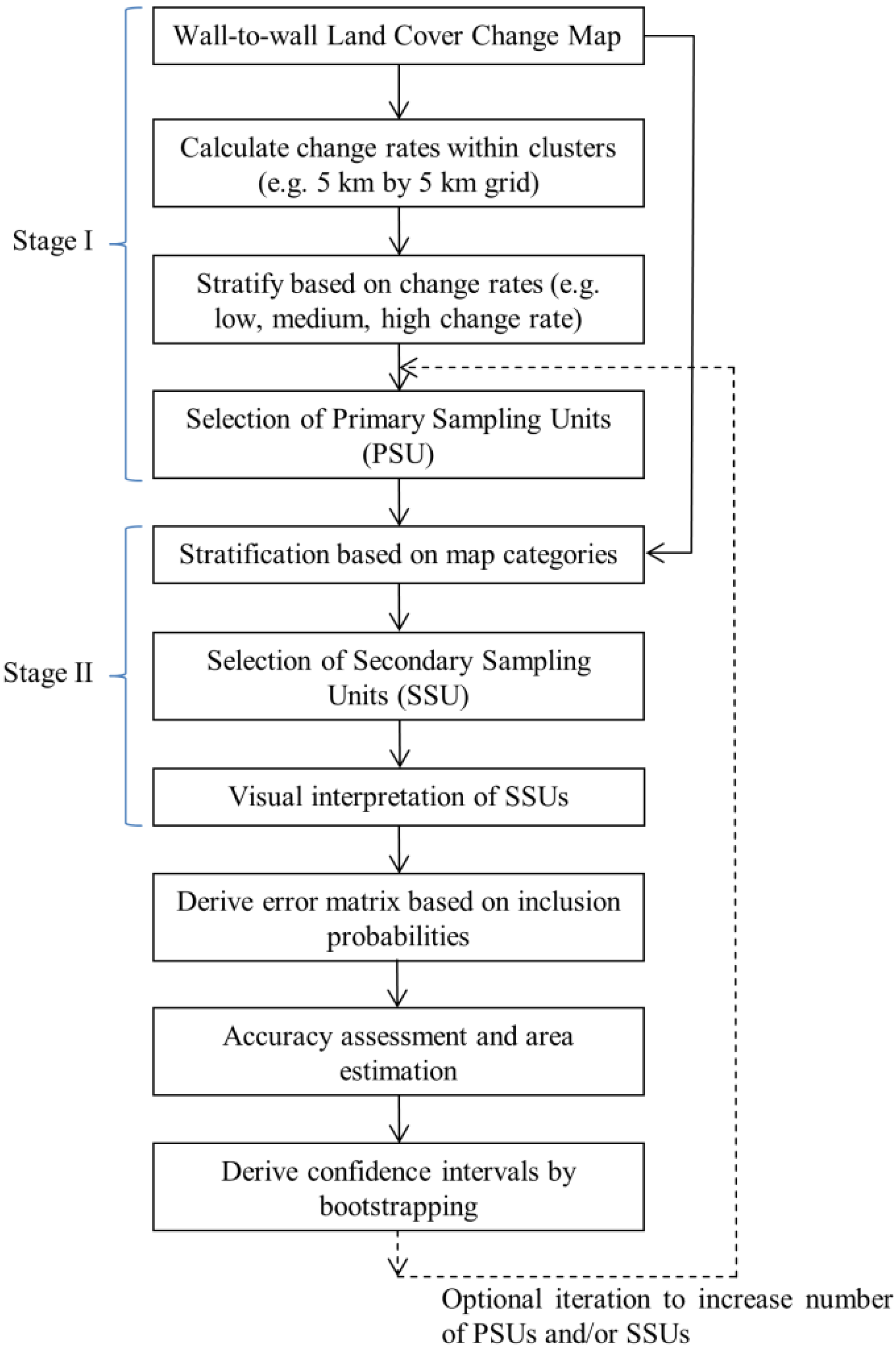
2.2. Sampling Design

A probability sampling design is a prerequisite for providing a rigorous foundation for the accuracy assessment and area estimation. The two conditions defining probability sampling are that the inclusion probability must be known for each unit selected in the sample and the inclusion probability must be greater than zero for all units in the population [11]. The inclusion probability for a unit is thereby defined as the probability that this unit (e.g., a pixel in the application example described below) is included in the sample.For operational applications over large areas, however, this cannot always be fully achieved, e.g., in the application example of the current project, frequent cloud cover leads to missing reference data for specific locations. In the example application we therefore allow limited shifting in the primary sampling units’ selection process, as described in Section 3. Under the assumption of random distribution of cloud cover at the local level, this introduces a small non-sampling error.
Based on the objectives and requirements specified in the introduction, we propose a two-stage stratified sampling design as outlined in Figure 1. Wall-to-wall maps on land cover changes are used as input.
In the first stage, stratified random sampling is applied to select the primary sampling units (PSUs). The primary sampling units are blocks which are covered with remote sensing imagery with significantly improved information content compared to the data used to derive the land cover change maps. The land cover changes to be monitored often affect only small portions of the total area, or they are spatially clustered over the region of interest. Only a limited number of very high resolution remote sensing scenes should be required for operational applications because of data acquisition and data processing cost. Stratification is therefore applied by using the land cover change map as described, for example, in [6].The change magnitude is calculated for each block, and the block is then assigned to one of the strata based on the percent area of changes, as described, e.g., in [12], where all blocks are associated to one of three strata based on the percent area of forest cover loss. The number of PSUs required depends mainly on the classification accuracy, the spatial pattern of the land cover, the spatio-temporal pattern of the land cover changes, the magnitude of the changes, and the required accuracy of the area estimates. As described in [6], sample size planning is inexact because it is dependent on accuracy and area information that must be estimated prior to conducting the actual accuracy assessment. However, an iterative procedure can be applied by specifying the number of primary and secondary sampling units based on comparable applications for the first iteration. The sample size allocation process can then be iterated until an allocation is found that yields satisfactory, anticipated standard errors for the key accuracy and area estimates [6].
In the second stage, stratified random sampling is applied to select the secondary sampling units (SSUs) with the pixel as the spatial assessment unit. To gain control over rare land cover change classes, stratification is performed based on the map classes that are validated as described, e.g., by [6] or [10]. This involves assigning all pixels within the sampled PSUs to strata based on the land cover change map categories. Stratified random sampling is then performed to select the secondary sampling units within each category. The allocation of the number of SSUs for the different strata depends on the specified monitoring objectives. Neyman optimal allocation is advantageous for estimating the area of change as well as overall accuracy, whereas equal allocation (same number of SSUs in each stratum) is advantageous for estimating the error of commission (compare, e.g., [13]).
Practical applications require accurate area estimation as well as accurate determination of the overall accuracy and of errors of commission and of omission. In a first step we therefore determine the minimum number of SSUs required for an accepted standard error of the error of commission per category according to [14] with:
n c =   p c ( 1 p c ) σ c 2  ,  c = 1 , , L
  • n c  number of SSUs for category c
  • p c  estimated error rate for category c
  • σ c  accepted standard error of the error of commission for category c
  • L   number of categories
For an accepted standard error of the error of commission of 0.05 and a conservatively estimated error rate of 0.50, a minimum sample size of nc = 100 SSUs results from this equation. In the demonstration application described below, a minimum number of nc = 100 SSUs (pixels) is therefore sampled within each land cover category. However, focusing on the error of commission only, by using an equal distribution of nc = 100 SSUs for all land cover change strata, would weaken the statistical analyses of the unchanged area, as land cover changes in most applications are rare (below several percent of the total area). In other words, the large unchanged area would be sampled with few SSUs in relation to its proportion, which impedes the detection of omission errors. To overcome this problem, additional SSUs are allocated according to Neyman optimal allocation, which minimizes the variance of the estimator of overall accuracy for a given total sample size n with [13]:
n c = n N c σ c k = 1 L N k σ k
  • n c  sample size for category c
  • n   total sample size
  • N c  population size for category c
  • σ c  estimated error rate for category c
  • L     number of categories
  • Nk population size for category k
  • σk  estimated error rate for category k
The result of this procedure is an uneven distribution of the number of SSUs in the different strata, however, with a defined minimum number of SSUs per stratum, as described above. The definition of the sampling units as points, pixels, polygons with a specified minimum mapping unit, etc. depends on the specific application. An example implementation is described in the next section.
As for the selection of the PSUs, an iterative procedure can be applied where, in a first iteration, a low total number of SSUs are randomly sampled. A decision as to whether the total number of SSUs needs to be increased in a next iteration can then be made based on the resulting confidence intervals for the area estimates and the estimated error measures.

2.3. Accuracy Assessment

By taking into account economic constraints, the primary and secondary sampling units are used for accuracy assessment, for area estimation, and for computation of the confidence intervals in one consistent approach. An error matrix is generated based on the inclusion probability for each sampled pixel as a basis for all subsequent processing steps [15]. The rows of the error matrix represent the labels shown in the map and the columns represent the labels depicted in the reference data. The inclusion probability is thereby defined as the probability that a pixel is included in the sample. If the total number of blocks in a stratum h is denoted as Kh, the first-stage sample inclusion probability for each block in stratum h is π1h = B1h/Kh, with B1h as the number of the selected blocks (PSUs) in stratum h. The second-stage inclusion probability is given by π2ch = nch/Nch with nch as the number of the sampled pixels (SSUs) for category c in stratum h and Nch as the total number of pixels classified as category c in stratum h.
The final inclusion probability for both stages together for pixel u in stratum h is the product of the inclusion probabilities at both stages [16].
π u c h * =   π 1 h * π 2 c h
To combine sample data over several strata, a weighted estimator of the error matrix is required to account for the different inclusion probabilities among the strata. The estimation weight is the inverse of each sample pixel’s inclusion probability. The proportion of area for each cell of the error matrix is thereby estimated by
p ^ i j =   ( 1 N ) x ( i , j ) 1 π u c h *
where N is the total number of pixels in the whole target region from which the sample is selected, and the summation is calculated over all sample pixels that meet the condition for entry into row i and column j of the error matrix (i.e., pixel u belongs to row i and column j). The result of this processing step is an error matrix which is based on inclusion probabilities and which directly gives the main accuracy parameters as described in the following. Once p ^ ij is computed for all cells of the error matrix, the overall accuracy is estimated by summing the p ^ ij values on the main diagonal of the error matrix [17]:
OA = j = 1 J p ^ jj
There are two more common accuracy measures. The error of commission (error of including an area in a category to which it does not truly belong, i.e., area overestimation) is estimated as:
E C ^ j = 1 p ^ j j i = 1 J p ^ i j
The error of omission (error of excluding an area from a category to which it truly belongs, i.e., area underestimation) is estimated as:
E O ^ i = 1 p ^ i i j = 1 J p ^ i j

2.4. Area Estimation

As described in the introduction, errors of omission and errors of commission are, in general, not equal, and the resulting bias is adjusted on the basis of the accuracy assessment. As the proposed approach uses probability sampling and the error matrix is based on inclusion probabilities, accuracy and area estimates can be computed directly from the error matrix. As each cell gives the unbiased estimator of the proportion of area, the area proportions for each reference-defined category j are estimated directly from the column totals ( p ^ j ). An unbiased estimator of the total area of category j is then [4]:
A ^ j = A t o t   ×   p ^ j
with A t o t being the total mapped area.
This estimator can be viewed as an “error adjusted” area estimator because it includes the area of map omission error of category j and leaves out the area of commission error. Although the area of estimated change is based on the reference sampling units, the map is an important component of the area estimation approach because of the role of the derived inclusion probabilities in the area estimator and the importance of stratification defined by the map classification [4].
The same information that is used for the accuracy assessment is therefore directly used to improve the area estimation by simply using the information provided by the error matrix.

2.5. Derivation of Confidence Intervals

Confidence intervals are derived in order to quantify the uncertainty of the accuracy measures and the area estimates. The confidence interval is a range that encloses the true (but unknown) value with a specified confidence (probability). For example, the 95% confidence interval has a 95% probability of enclosing the true value. In the proposed approach, bootstrapping is applied for derivation of the confidence intervals as, e.g., described in [18,19], where the selection of the bootstrap samples emulates the actual sample selection method. Bootstrapping is thus performed by repeated sampling of the PSUs and SSUs from the whole sample set with replacement. In the application example described in the next section, we selected 200 runs in the first phase and 200 runs in the second phase, which leads to a total of 40,000 runs.
As described in [19], the percentile method interval is used for estimating the confidence intervals. The percentiles are estimated directly on the basis of the bootstrap distribution. For 95% confidence intervals, for example, the interval between 2.5% and 97.5% of the bootstrap quantiles is determined. All elements of the error matrix p ^ i j as well as the derived accuracy measures and the area estimates are calculated in each of the runs. With this bootstrapping approach, confidence limits around the derived overall accuracy, error of omission, and error of commission, as well as around the area estimates, are derived by treating the B samples as independent estimates of the same quantities. For example, the 95% confidence interval for the estimated overall accuracy is derived from the 2.5% to 97.5% quantile of the bootstrap distribution. Compared to the often-applied α percentiles of the standard normal distribution, the main advantage is that no assumption on normal distribution is required. In the next section some figures illustrate the procedure based on the application example.

3. Results of a Case Study for Monitoring Deforestation

The following example illustrates the workflow for monitoring tropical deforestation in the Republic of Congo in the frame of REDD (Reducing Emissions from Deforestation and Forest Degradation) reporting. To demonstrate the cost-effective operational applicability of the approach, we selected a study site characterized by frequent cloud cover and very low deforestation rates, which makes deforestation monitoring particularly challenging.

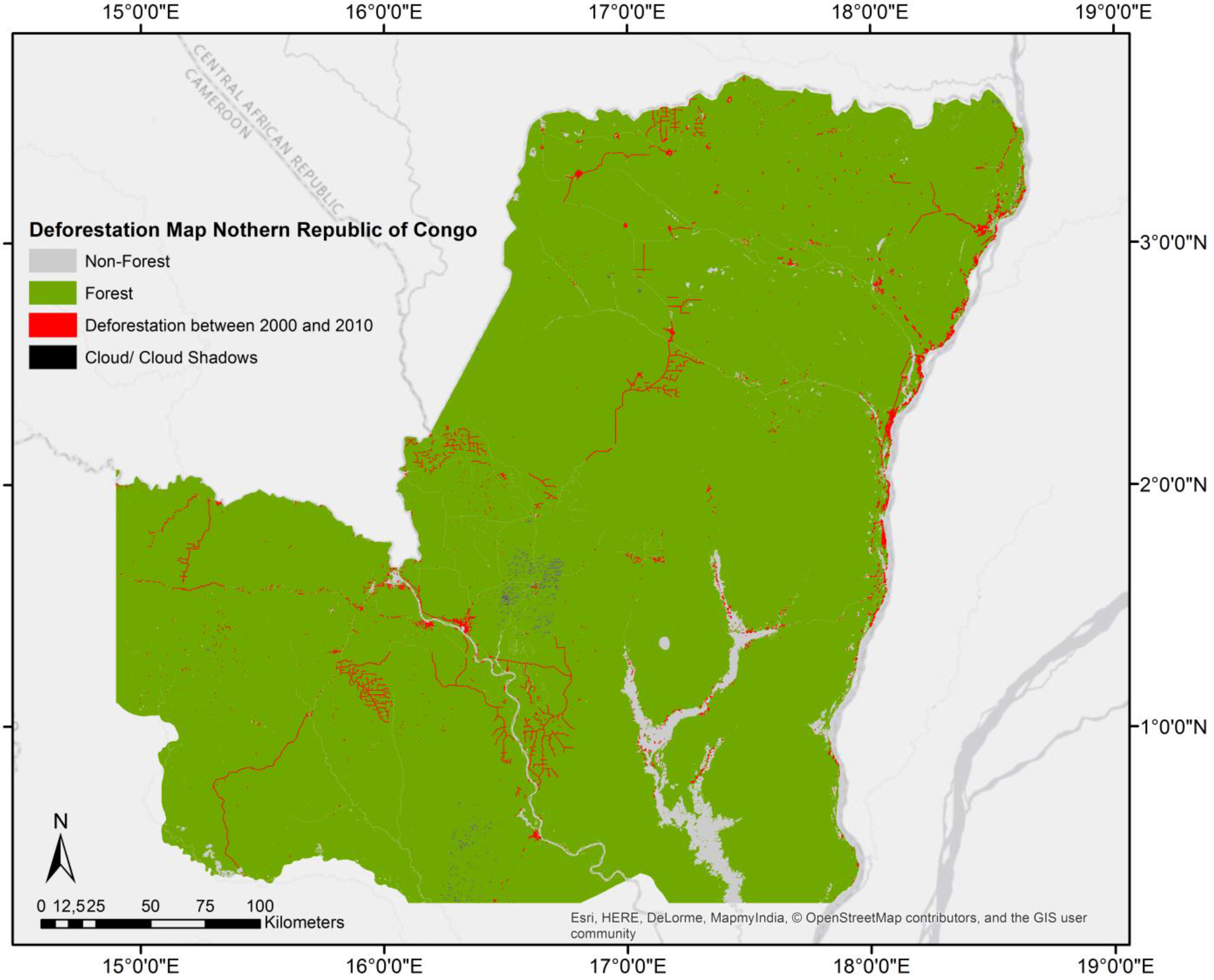
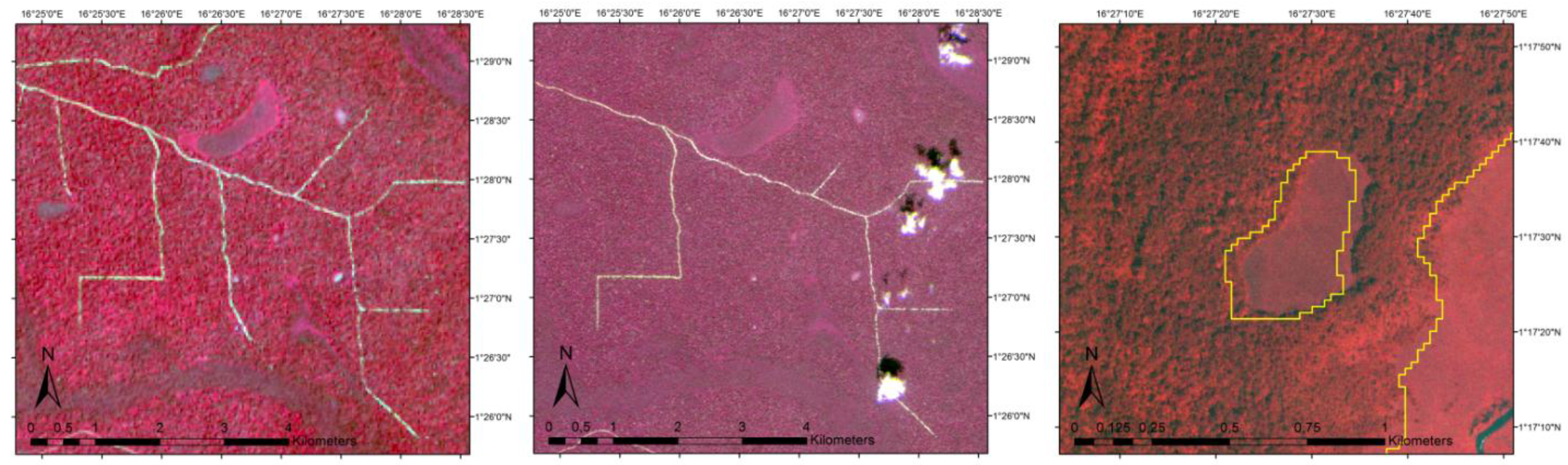
3.1. Study Site and Data

The study site is located in the northern part of the Republic of Congo. It is dominated by tropical rainforests covering more than 95% of the area and is one of the cloudiest regions in Africa. Deforestation occurs at very low rates and is concentrated close to settlements along rivers and roads. A sufficiently large area of 100,000 km2 was selected to demonstrate the operational applicability of the approach for large areas. A deforestation map derived from Landsat 5 Thematic Mapper (TM) and Landsat 7 Enhanced Thematic Mapper (ETM) imagery for the period 2000 to 2010 with a spatial resolution of 30 m by 30 m per pixel was provided by project partner Gesellschaft für Angewandte Fernerkundung AG. An overview of the study site showing the location of the deforested areas (aggregated to one deforestation category) is shown in Figure 2.
Figure 2. Study site located in the northern part of the Republic of Congo with deforested areas highlighted in red.
Remotesensing 07 11992 g002
According to nomenclature specifications defined in [20], the categories “forest”, “non-forest”, change from “forest to cropland”, “forest to grassland”, “forest to wetland”, and “forest to settlement” were mapped. As pre-processing steps, the project partner Gesellschaft für Angewandte Fernerkundung AG relatively calibrated the ortho-rectified satellite images to generate blocks consisting of several scenes which were processed together. They applied a semi-automatic classification procedure for generating the land cover change map where, in a first step, automated change detection was performed, and in a second step, the change detection results were revised by visual interpretation.
For accuracy assessment and area estimation, very high resolution (VHR) and high resolution (HR) archive imagery was available (see Table 1). In the context of the current application example, VHR refers to satellite images with a spatial resolution of at least 5 m per picture element, whereas HR refers to satellite images with a spatial resolution in the range of 5 m to 30 m.
The European Space Agency (ESA) provided ortho-rectified, multi-temporal HR satellite images from SPOT, ASTER, and RapidEye via their data warehouse free of cost. The Airbus Defence and Space company provided a VHR Pléiades scene free of charge. Landsat 7 data were downloaded from USGS servers free of cost. In addition, IKONOS-2 and GeoEYE satellite data acquired in 2009 and 2011 (5 km by 5 km frames) was purchased for the project, according to the sampling requirements described below.
Table 1. Satellite scenes used for accuracy assessment and area estimation (pan for panchromatic and ms for multispectral data).
Satellite SensorSpatial ResolutionAcquisition YearsNumber of Scenes
GeoEye-10.5 m (pan), 2 m (ms)2009–201112
Ikonos-21 m (pan), 4 m (ms)2009–201112
Rapideye MSI5 m (ms)2009–20116
Landsat TM and ETM15 m (pan), 30 m (ms)2000–201346
Spot 4 HRVIR20 m (ms)2000, 20015
Spot 5 HRG10 m (ms)2009, 20103
Terra Aster15 m (ms)2007, 20102
Pléiades HiRI0.5 m (pan), 2 m (ms)20131

3.2. Sampling Design

As described above, two-stage stratified random sampling was applied. In the first stage, n = 32 area frames were selected as primary sampling units, which is comparable to other approaches, e.g., [21], who selected n = 31 primary sampling units for assessing the accuracy of the Alaska National Land Cover Database. For stratification into the categories of low, medium, and high change magnitude, the mean deforestation rate was calculated for 10 km by 10 km blocks on the basis of the deforestation map. The selection of the PSUs for each of the three strata was then performed by random sampling. By taking into account cloud and cloud-shadow problems and the extent of VHR archive satellite scenes, we used the 10 km by 10 km blocks, within which the selected area frames were shifted. Our primary sampling units (PSUs) are therefore 5 km by 5 km area frames, which are shifted within the 10 km by 10 km blocks. In addition to the VHR satellite data, multi-temporal HR satellite data was also available for each area frame as described above. For retrospective monitoring of land cover changes for which archive imagery is required, we recommend this procedure of shifting within blocks, especially for areas characterized by frequent cloud cover. However, for monitoring current/future land cover changes, tasking of satellite acquisitions such as, e.g., for Pléiades acquisitions can be recommended, if possible within cost constraints.
In the second stage, a set of pixels (secondary sampling units or SSUs) were randomly sampled within the VHR satellite scenes with the wall-to-wall deforestation map being used for stratification. The number of sampled pixels was determined according to Equation (1) for a conservatively estimated error rate of 0.50 and an accepted standard error of the error of commission of 0.05, with a minimum sample size of n = 100 pixels per stratum. As described above, such equal distribution of n = 100 SSUs for each stratum would weaken the statistical analyses of the unchanged area, as the large unchanged area would be sampled with few SSUs in relation to its proportion. To overcome this problem, additional SSUs were allocated using Neyman optimal allocation as defined in Equation (2), for a priori estimated error rates of 3% for forest, 10% for non-forest, and 50% for the deforestation categories. This results in an allocation of n = 4015 pixels to the category “unchanged forest” and n = 377 pixels to the category “unchanged non-forest”. For the deforestation categories, a total of n = 208 pixels would be allocated using Neyman optimal allocation. As specified above, however, a minimum of n = 100 pixels is allocated to each of the deforestation categories. A total of n = 4792 SSUs was therefore randomly sampled within the respective strata.
Figure 3. Example of a six-month time lag between a Landsat ETM scene (left image) and a RapidEye scene (center image), and example of a geometric shift between a reference scene and the provided forest map (highlighted in yellow), seen in the right image.
Remotesensing 07 11992 g003
For each SSU, the reference category was visually interpreted on the basis of the VHR data and the high resolution satellite time series including the production scenes. Time lags and geometric shifts were taken into account in the interpretation process, e.g., a sampling unit was not labeled as erroneous if a geometric shift was observed between the VHR reference data and the deforestation map and the deforestation was detected correctly (see Figure 3).
The resulting information on the classified and reference categories for each SSU was then used for accuracy assessment as well as for estimating the area of deforestation including the estimation of confidence intervals.

3.3. Accuracy Assessment

For all subsequent processing steps, an error matrix was generated based on the inclusion probabilities as defined in Equations (3) and (4). The rows of the error matrix represent the labels shown in the deforestation map and the columns represent the labels depicted in the reference data (see Table 2 and Table 3). The diagonal entries represent correct classifications, or agreement, between the map and reference data, and the off-diagonal entries represent misclassifications.
Table 2. Error matrix based on inclusion probabilities.
ReferenceStable Non-ForestStable ForestForest to CroplandForest to GrasslandForest to WetlandForest to Settlement
Map
Stable non-forest0.02230.00470.00040.00000.00000.0000
Stable forest0.00280.96310.00290.00000.00000.0009
Forest to cropland0.00000.00010.00100.00000.00000.0000
Forest to grassland0.00000.00030.00000.00020.00000.0000
Forest to wetland0.00000.00000.00000.00000.00010.0000
Forest to settlement0.00000.00010.00010.00000.00000.0010
Total0.02510.96830.00440.00020.00010.0019
Table 3. Error of commission and omission in percent.
Stable Non-ForestStable ForestForest to CroplandForest to GrasslandForest to WetlandForest to Settlement
Error of commission18.80.78.560.839.718.2
Error of omission11.10.577.912.949.349.6
The accuracy assessment shows a high overall accuracy of 98.8%. As shown in Table 2, this high overall accuracy is due to the highly accurate mapping of the dominating category “stable forest”, whereas the errors of omission and commission are high for the deforestation categories. This is expected as Landsat TM imagery with a spatial resolution of 30 m per pixel was used for deforestation mapping and deforestation within the study site occurs mostly on small patches, such as, e.g., the extension of settlements at the border with small housing units.

3.4. Area Estimation

Accurate estimation of the area undergoing land cover changes is an important prerequisite for fulfilling REDD reporting requirements. As clearly stated in the Good Practice Guidance for Land Use, Land Use Change and Forestry [20]: “Estimates should be accurate in the sense that they are systematically neither over nor under true emissions or removals, so far as can be judged, and that uncertainties are reduced so far as is practicable”. As described above, errors of omission and errors of commission are, in general, not equal, which leads to systematic over- or underestimation of the true area. For the category “change from forest to settlement”, the error matrix in Table 2 shows, e.g., that a fraction of 0.1% of the total area is classified correctly as change from “forest to settlement”, a fraction of 0.09% is classified incorrectly as “stable forest” instead of “change from forest to settlement”, a fraction of 0.01% is classified incorrectly as “change from forest to settlement” instead of “stable forest” and a fraction of 0.01% is classified incorrectly as “forest to settlement” instead of “forest to cropland”.
Whereas, according to the deforestation map, a fraction of 0.12% of the total area is mapped as change from “forest to settlement” (the row total in the error matrix, expressed in percent), the improved area estimate taking into account the over- und underestimations shows that a fraction of 0.2% changed from forest to settlement (the column total in the error matrix, expressed in percent). By applying Equation (8), improved area estimates are therefore derived simply by multiplying the total mapped area with the column totals of the error matrix. Table 4 shows that the improved area estimates significantly differ from the mapped areas, e.g., according to the map, changes from forest to settlement occurred in an area of 117 km2, whereas the area estimated on the basis of the error matrix is 191 km2. This significant underestimation of the area of change from “forest to settlement” in the deforestation map is caused by small housing units, which cannot be detected well with Landsat TM imagery because of the relatively low spatial resolution of 30 m per pixel.
Table 4. Area estimates (area in km2) and upper and lower bounds at the 95% confidence interval.
CategoryMapped Area in km2Improved Area Estimates in km2Lower Bound (95% Confid.)Upper Bound (95% Confid.)
Non-forest2661244213042933
Forest94396942609392695595
Forest to cropland1004261051094
Forest to grassland4520634
Forest to wetland2010020
Forest to settlement11719194360

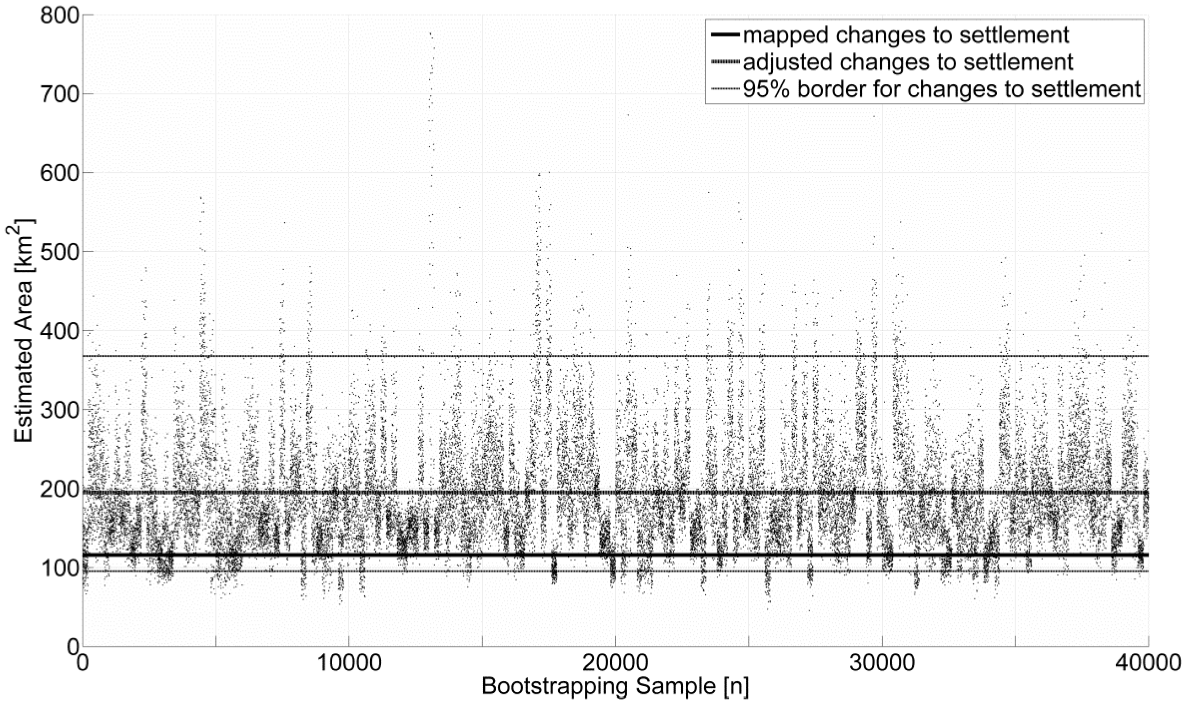
3.5. Derivation of Confidence Intervals

A 95% confidence interval is normally used for estimation of emissions and removals under the United Nations Framework Convention on Climate Change [3]. The 95% confidence interval has a 95% probability of enclosing the true but unknown value of the parameter. The 95% confidence interval is enclosed by the 2.5th and 97.5th percentiles of the probability density function. These percentiles are estimated directly on the basis of the bootstrap distribution by applying 200 runs for selecting the PSUs in the first phase, and within each of these runs, applying 200 runs for selecting the SSUs, which leads to a total of 40,000 runs. Figure 4 shows the results of these 40,000 runs for estimating the area of change from forest land to settlement. As stated above, the deforestation map indicates an area of 117 km2, whereas the area estimated by bootstrapping is 191 km2, with a range between 94 km2 and 360 km2 at the 95% confidence interval. Please note that the bootstrap distribution as shown in Figure 4 is non-Gaussian, with asymmetric confidence intervals.
The bootstrapping results show an overall accuracy of 98.8% and a range of the overall accuracy between 97.6% and 99.3% at the 95% confidence level. Table 4 shows the area estimates including the confidence intervals as required for REDD reporting.
Figure 4. Bootstrapping for estimating area of change from forest land to settlement, with n = 200 runs for first-phase sampling and n = 200 runs for second-phase sampling.
Remotesensing 07 11992 g004

4. Discussion

Sectorial monitoring of selected land cover change processes is already performed operationally. For example, national forest inventories have for decades provided accurate data for the forestry sector in developed countries. Several operational land cover change monitoring programs have been put in place by the European Union, ESA, NASA, FAO, universities, and others, which provide valuable information on land cover changes. The data, however, is often provided at low spatial or low temporal resolution or at low accuracy levels or for specific sectors only, and is often not provided up-to-date. When taking into account the tremendous impacts that land cover changes cause from the local to the global level, current operational monitoring systems are inadequate in providing all required information. Free availability of dense time series data from Sentinel-2 with increased temporal, spatial, and spectral resolution compared to current freely available data such as, e.g., from the Landsat satellite series, and the availability of very high resolution satellite imagery at moderate cost will improve this situation significantly.
Accurate monitoring of land cover changes is especially challenging when the change rate is very low, such as in the application example, where the change from forest to settlement was only 0.2%. However, such low change rates are typical for many applications. The accuracy of land cover change maps is often not sufficient to provide accurate estimates for change processes with such low change rates. Several methods were therefore developed to complement land cover change maps with a sampling approach for accuracy assessment, improved area estimation, and derivation of confidence intervals as required, for example, in international reporting.
For one-stage sampling approaches, e.g., simple random sampling or stratified sampling, analytic formulas for accuracy assessment and derivation of confidence intervals have been published, e.g., by [4,5,13,22]. In these sampling approaches, however, processing of a large number of VHR satellite scenes would be required, as the sampling units are not grouped spatially into clusters. For most land cover change monitoring applications, the acquisition dates of the VHR satellite scenes must also be within pre-defined time intervals. This limits the applicability of, e.g., Google Earth or related services, as acquisition dates and VHR coverage of these services strongly depend on financial constraints. In cases where VHR satellite imagery is already provided on a wall-to-wall basis within required time intervals, wall-to-wall mapping of land cover changes would be possible, but is often out of scope due to constraints in terms of cost and implementation time. However, one-stage stratified sampling can be recommended in this case. As, in general, such data is not available, two-stage sampling can be implemented, as proposed in the present approach.
When using a sampling scheme with more than one stage, standard errors of the accuracy estimators depend on the specific sampling design implemented at each stage. As a practical approach to estimating standard errors in such a sampling scheme, the design is often treated as if it were a one-stage cluster sample with the clusters selected by simple random sampling, where the inclusion probability for any pixel is calculated as the product of probabilities for each stage [21]. Approximate equations for the associated accuracy statistics and standard errors are usually given in such cases, e.g., in [21,23]. Instead of applying such approximate and highly complex equations, which are often based on normal distribution assumptions, the current approach uses bootstrapping, as confidence intervals can be constructed without having to make normal theory assumptions [18]. The main drawback of the current approach lies in the added complexity for stratification within the cluster sampling design. Specifically, the number of the required primary sampling units needs to be estimated, as it depends on accuracy and area information, which is not known prior to the actual accuracy assessment. However, the number of primary sampling units can be increased iteratively, until an allocation is found that yields satisfactory anticipated standard errors for the key accuracy and area estimates [6].
The area estimates and verification estimations rely on a high quality visual interpretation of the sampling units based on time series of satellite imagery.

5. Conclusions

We propose a cost-effective approach to complement land cover change maps with a sampling approach, which is used for accuracy assessment and accurate estimation of areas undergoing land cover changes, including provision of confidence intervals. In order to keep accuracy, efficiency, and effort of the estimations in balance, stratification is applied in both stages of the sampling approach, which targets the following specific requirements:
  • General applicability for a wide range of operational applications
  • Cost-effective implementation for large-area monitoring
  • Based on globally available data (e.g., freely available Sentinel 2 imagery, complemented with a limited number of very high resolution scenes)
  • Accurate monitoring of typically rare land cover change processes (e.g., change rates below 1%)
  • Implementation of a probability sampling design to provide a rigorous foundation for accuracy assessment and area estimation
  • Provision of confidence intervals for accuracy measures as well as area estimates as required in international reporting.
The application of the approach for assessment of deforestation in an area characterized by frequent cloud cover and very low change rate in the Republic of Congo demonstrates that these targets are achieved, even under particularly challenging monitoring conditions.

Acknowledgments

This study was funded under the European Space Agency’s (ESA) GSE Forest Monitoring project coordinated by Gesellschaft für Angewandte Fernerkundung AG as part of the Global Monitoring for Environment and Security Services Element. The authors would like to thank the referees for their constructive reviews that improved the manuscript significantly.

Author Contributions

All authors have made major and unique contributions. Heinz Gallaun, the main author, was responsible for method development, designed the workflow and wrote the draft version of the manuscript. Martin Steinegger implemented the methods and processed the statistical analysis. Martin Steinegger, Ursula Schmitt and Roland Wack generated the reference data and gave valuable inputs on the manuscript writing. Mathias Schardt and Birgit Kornberger provided valuable inputs on statistical methods.

Conflicts of Interest

The authors declare no conflict of interest.

References

  1. Tewkesbury, A.P.; Comber, A.J.; Tate, N.J.; Lamb, A.; Fisher, P.F. A critical synthesis of remotely sensed optical image change detection techniques. Remote Sens. Environ. 2015, 160, 1–14. [Google Scholar] [CrossRef]
  2. Hussain, M.; Chen, D.; Cheng, A.; Wei, H.; Stanley, D. Change detection from remotely sensed images: From pixel-based to object-based approaches. ISPRS J. Photogramm. Remote Sens. 2013, 80, 91–106. [Google Scholar] [CrossRef]
  3. GOFC-GOLD. A Sourcebook of Methods and Procedures for Monitoring and Reporting Anthropogenic Greenhouse Gas Emissions and Removals Associated with Deforestation, Gains and Losses of Carbon Stocks in Forests Remaining Forests, and Forestation, GOFC-GOLD Report version COP20–1; GOFC-GOLD Land Cover Project Office: Wageningen, The Netherlands, 2014. [Google Scholar]
  4. Olofsson, P.; Foody, G.M.; Stehman, S.V.; Woodcock, C.E. Making better use of accuracy data in land change studies: Estimating accuracy and area and quantifying uncertainty using stratified estimation. Remote Sens. Environ. 2013, 129, 122–131. [Google Scholar] [CrossRef]
  5. Card, D.H. Using known map category marginal frequencies to improve estimates of thematic map accuracy. Am. Soc. Photogramm. 1982, 48, 431–439. [Google Scholar]
  6. Olofsson, P.; Foody, G.M.; Herold, M.; Stehman, S.V.; Woodcock, C.E.; Wulder, M.A. Good practices for estimating area and assessing accuracy of land change. Remote Sens. Environ. 2014, 148, 42–57. [Google Scholar] [CrossRef]
  7. Sannier, C.; McRoberts, R.E.; Fichet, L.-V.; Makaga, E.M.K. Using the regression estimator with Landsat data to estimate proportion forest cover and net proportion deforestation in Gabon. Remote Sens. Environ. 2014, 151, 138–148. [Google Scholar] [CrossRef]
  8. McRoberts, R.E.; Walters, B.F. Statistical inference for remote sensing-based estimates of net deforestation. Remote Sens. Environ. 2012, 124, 394–401. [Google Scholar] [CrossRef]
  9. McRoberts, R.E. Post-classification approaches to estimating change in forest area using remotely sensed auxiliary data. Remote Sens. Environ. 2014, 151, 149–156. [Google Scholar] [CrossRef]
  10. Stehman, S.V. Sampling designs for accuracy assessment of land cover. Int. J. Remote Sens. 2009, 30, 5243–5272. [Google Scholar] [CrossRef]
  11. Stehman, S.V. Statistical rigor and practical utility in thematic map accuracy assessment. Photogramm. Eng. Remote Sens. 2001, 67, 727–734. [Google Scholar]
  12. Hansen, M.C.; Stehman, S.V.; Potapov, P.V.; Arunarwati, B.; Stolle, F.; Pittman, K. Quantifying changes in the rates of forest clearing in Indonesia from 1990 to 2005 using remotely sensed data sets. Environ. Res. Lett. 2009, 4, 034001. [Google Scholar] [CrossRef]
  13. Stehman, S.V. Impact of sample size allocation when using stratified random sampling to estimate accuracy and area of land-cover change. Remote Sens. Lett. 2012, 3, 111–120. [Google Scholar] [CrossRef]
  14. Bossard, M.; Feranec, J.; Otahel, J. CORINE Land Cover Technical Guide: Addendum 2000; European Environment Agency Copenhagen: Copenhagen, Denmark, 2000. [Google Scholar]
  15. Selkowitz, D.J.; Stehman, S.V. Thematic accuracy of the National Land Cover Database (NLCD) 2001 land cover for Alaska. Remote Sens. Environ. 2011, 115, 1401–1407. [Google Scholar] [CrossRef]
  16. Särndal, C.-E.; Swensson, B.; Wretman, J. Model Assisted Survey Sampling; Springer Science & Business Media: Berlin, Germany, 2003. [Google Scholar]
  17. Foody, G.M. Sample size determination for image classification accuracy assessment and comparison. Int. J. Remote Sens. 2009, 30, 5273–5291. [Google Scholar] [CrossRef]
  18. Schreuder, H.T.; Ernst, R.L.; Ramirez-Maldonado, H. Statistical Techniques for Sampling and Monitoring Natural Resources; General Technical Report RMRS-GTR-126; U.S. Department of Agriculture, Forest Service, Rocky Mountain Research Station: Fort Collins, CO, USA, 2004.
  19. Efron, B.; Tibshirani, R. Bootstrap methods for standard errors, confidence intervals, and other measures of statistical accuracy. Stat. Sci. 1986, 1, 54–75. [Google Scholar] [CrossRef]
  20. Penman, J.; Gytarsky, M.; Hiraishi, T.; Krug, T.; Kruger, D.; Pipatti, R.; Buendia, L.; Miwa, K.; Ngara, T.; Tanabe, K. Good Practice Guidance for Land Use, Land-Use Change and Forestry; Institute for Global Environmental Strategies (IGES): Kanagawa Hayama, Japan, 2003. [Google Scholar]
  21. Stehman, S.V.; Selkowitz, D.J. A spatially stratified, multi-stage cluster sampling design for assessing accuracy of the Alaska (USA) National Land Cover Database (NLCD). Int. J. Remote Sens. 2010, 31, 1877–1896. [Google Scholar] [CrossRef]
  22. Olofsson, P.; Torchinava, P.; Woodcock, C.E.; Baccini, A.; Houghton, R.A.; Ozdogan, M.; Zhao, F.; Yang, X. Implications of land use change on the national terrestrial carbon budget of Georgia. Carbon Balance Manag. 2010, 5. [Google Scholar] [CrossRef] [PubMed]
  23. Stehman, S.V. Estimating standard errors of accuracy assessment statistics under cluster sampling. Remote Sens. Environ. 1997, 60, 258–269. [Google Scholar] [CrossRef]

