The Impact of the Calibration Method on the Accuracy of Point Clouds Derived Using Unmanned Aerial Vehicle Multi-View Stereopsis

Abstract

In unmanned aerial vehicle (UAV) photogrammetric surveys, the camera can be pre-calibrated or can be calibrated “on-the-job” using structure-from-motion and a self-calibrating bundle adjustment. This study investigates the impact on mapping accuracy of UAV photogrammetric survey blocks, the bundle adjustment and the 3D reconstruction process under a range of typical operating scenarios for centimetre-scale natural landform mapping (in this case, a coastal cliff). We demonstrate the sensitivity of the process to calibration procedures and the need for careful accuracy assessment. For this investigation, vertical (nadir or near-nadir) and oblique photography were collected with 80%–90% overlap and with accurately-surveyed ($\sigma \le$ 2 mm) and densely-distributed ground control. This allowed various scenarios to be tested and the impact on mapping accuracy to be assessed. This paper presents the results of that investigation and provides guidelines that will assist with operational decisions regarding camera calibration and ground control for UAV photogrammetry. The results indicate that the use of either a robust pre-calibration or a robust self-calibration results in accurate model creation from vertical-only photography, and additional oblique photography may improve the results. The results indicate that if a dense array of high accuracy ground control points are deployed and the UAV photography includes both vertical and oblique images, then either a pre-calibration or an on-the-job self-calibration will yield reliable models (pre-calibration RMSE${}_{XY}$ = 7.1 mm and on-the-job self-calibration RMSE${}_{XY}$ = 3.2 mm). When oblique photography was excluded from the on-the-job self-calibration solution, the accuracy of the model deteriorated (by 3.3 mm horizontally and 4.7 mm vertically). When the accuracy of the ground control was then degraded to replicate typical operational practice (σ = 22 mm), the accuracy of the model further deteriorated (e.g., on-the-job self-calibration RMSE${}_{XY}$ went from 3.2–7.0 mm). Additionally, when the density of the ground control was reduced, the model accuracy also further deteriorated (e.g., on-the-job self-calibration RMSE${}_{XY}$ went from 7.0–7.3 mm). However, our results do indicate that loss of accuracy due to sparse ground control can be mitigated by including oblique imagery.

1. Introduction

The optimal workflow for high accuracy three-dimensional (3D) reconstruction using unmanned aerial vehicles (UAVs) (also known as remotely-piloted aircraft systems (RPAS) or drones) is the underlying motivation for much of the current research surrounding the use of photogrammetric, structure-from-motion (SfM) and multi-view stereopsis (MVS) techniques [1,2,3,4,5,6,7,8,9,10,11] with UAV imagery (UAV-MVS). This study is part of the research focussing on the application of UAV-MVS for mapping natural landform changes [12]. UAV-MVS has the potential to produce high accuracy 3D point clouds and digital surface models (DSMs), provided the workflow used in the data capture and processing is robust. Initial research has shown that the technique is capable of producing accuracies in the order of 25–40 mm when flying at 25–50 m above ground level (AGL) [12], but these findings do not show how accurate the technique could be under optimal survey design conditions. Quantification of positional accuracy is key to detecting and attributing centimetre-scale landform change.

The study site chosen for this research is a sheltered coastline that is eroding gradually. Prahalad et al. [13] suggest that although typical erosion rates along sheltered coasts are in the range of 10–20 cm/year the impact of single events contributing to this erosion cannot reliably be measured using satellite imagery or aerial photography and only becomes evident when a number of events have caused cumulative erosion. UAV-MVS may offer the ability to monitor small changes at temporal resolutions suited to the requirement for pre- and post-event mapping and at spatial resolutions of higher than 1–3 cm, allowing researchers to gain new understandings of these processes at the resolution of single events.

Camera network design and the distribution and accuracy of ground control are key determinants of the mapping accuracy that can be achieved from UAV-MVS. A number of studies have compared SfM and MVS derived products to total station surveyed check points [12,14,15], to DGPS (Differential Global Positioning System) surveyed check points [16,17,18] and to LiDAR or terrestrial laser scanning [19,20,21,22,23]. Some have pre-calibrated the camera [14,17], and others have relied on self-calibration [12,15,18,23,24] or compared the two options [16,19,20]. While these studies provided guidance for those making operational decisions during survey design and implementation, our study builds on previous work by quantifying the impact of camera calibration on the accuracy of UAV-MVS point clouds. The assessment of UAV-MVS techniques using a precise total station survey ($\sigma \le$ 2 mm) of ground control and verification points has not been done to date, particularly in the context of natural landform mapping.

The magnitude of systematic and random errors in a point cloud derived from UAV-MVS will be influenced by camera specifications (sensor format, lens focal length, etc.), camera calibration accuracy, camera network geometry, the distribution and accuracy of ground control and the precision with which targets can be measured and matched. The majority of cameras used in recent years for UAV surveys have not been designed for photogrammetric accuracy [25]. Non-metric “prosumer” or consumer-grade digital cameras are a popular choice for UAV-MVS, because of their light weight and low cost. These cameras are not manufactured to the same standards as metric cameras, and as a result, they exhibit much greater magnitudes of distortion and instability [25,26,27,28]. These unstable calibration characteristics and potentially large lens distortions, if not reliably modelled, will impact 3D accuracy [29,30]. Some studies have used a zoom lens [12]; however, a fixed focal length prime lens is likely to be more stable [25]. It is important that a calibration is undertaken that will adequately model a camera and lens at a chosen focus and focal length. It is necessary to fix the focal length and focus for each calibration and, if necessary, to perform a calibration for each setting needed for mapping surveys [25,26]. Camera calibration is therefore an important component of the photogrammetric process.

Pre-calibration using an image set captured from a typical operating distance (flying height) and a convergent camera station network, processed independently of the survey imagery, can be used to derive camera calibration parameters. Alternatively, pre-calibration can be performed more easily using an image set acquired at close range using a calibration array, such as a pattern (e.g., a checker board), a 3D targeted object or a target field. In this case, the calibration is computed from images acquired at camera-to-target distances shorter than those of a typical UAV survey. In the case of an on-the-job self-calibration, the camera calibration is derived from image coordinates measured in the mapping photography and including the camera calibration parameters as unknowns in a self-calibrating bundle adjustment.

The simplest option for camera calibration is usually to include camera calibration parameters as unknowns in a self-calibrating bundle adjustment. Advances in automated feature identification and matching in recent years have enabled users of consumer-grade cameras to model distortion relatively easily using the self-calibration approach based on a minimal number of overlapping photographs. There is a risk that the camera calibration parameters are derived from a relatively low number of images and a relatively poor camera geometry. In this situation, there is an increased potential for projective coupling between the interior and exterior orientation parameters [25,27]. This means that, while the calibration may be sufficient for the network of images acquired for the particular mapping task, the distortion parameters derived in this way are generally considered specific to the dataset and not necessarily applicable to other image sets. Poorly-modelled camera calibration leads to model deformation, particularly if the camera network is comprised of traditional nadir photography in strips and blocks [16,27,28,30].

The accuracy of the measurements directly impacts the repeatability of data capture, and this, in turn, impacts change detection. If the aim of a camera calibration is to reuse the calibration in high accuracy applications, then the calibration must not be specific to a particular camera network. A robust, reusable photogrammetric pre-calibration requires a camera network design and target objects that provide a comprehensive geometric modelling of a camera’s image space, independent of the target scene [26,31]. Precisely-coordinated target arrays or engineered 3D target objects, often used in close-range photogrammetric applications, such as engineering metrology, are generally inappropriate for UAV 3D mapping applications, because it is prohibitive to manufacturer arrays that are large enough to accommodate camera fields of view at typical flying heights.

For precise UAV surveys, a deliberate choice needs to be made between the different options. When using the self-calibration approach, the flight plan needs to incorporate design elements that promote effective and robust self-calibration. The inclusion of oblique imagery has the potential to improve the camera model, to reduce model deformation and to improve modelling of complex 3D forms, particularly when coupled with a good control distribution and a target scene that contains objects that result in reliable image matching [16,27,28,30,32,33].

Our experience with analysing configuration requirements and assessing the accuracy of UAV-MVS for monitoring centimetre-scale landform change demonstrated a need to assess the sensitivity of the process to camera calibration procedures [12]. The choices made when incorporating the camera model (in particular lens distortion) into UAV-MVS processing and the impact of camera network design and calibration procedure choices on model accuracy is the focus of this study.

The objectives of this investigation are: (i) to evaluate the impact of the camera calibration method on the model accuracy, specifically comparing self-calibration methods and pre-calibration options; (ii) to ascertain if self-calibration can result in comparable accuracy to pre-calibration if there is an appropriate camera network design, ground control point (GCP) distribution and GCP survey method accuracy; (iii) to assess the impact of additional oblique imagery on a predominantly nadir self-calibration; and (iv) to assess the influence of GCP quality on point cloud accuracy by comparing a precise total station survey and a DGPS survey of GCPs.

2. Experimental Section

2.1. Study Site

The study site is a 50 m section of Pittwater Estuary, a sheltered estuarine waterway in southeastern Tasmania, Australia (Figure 1). For this study, a section of an erosion scarp was chosen as the focus area to evaluate the impact of calibration choices on derived UAV-MVS point clouds. The vegetation is characterised by coastal grasses along an erosion scarp with salt marsh at the southern end of the study site.

2.2. Hardware

The UAV used in this study was an OktoKopter UAV platform [34] with a Droidworx eight rotor airframe. The aircraft has an electric multi-rotor system and is capable of carrying a $\sim$2.5-kg payload for approximately 8–10 min. An on-board navigation-grade GPS (5–10 m positional accuracy), IMU, 3D digital compass and barometric altimeter allow the system to navigate to predefined waypoints. A Canon 550D digital SLR camera with a 20 mm prime lens was attached to a stabilised camera mount that allows camera tilt to be controlled by the UAV operator. This camera has a lightweight body and provides control over ISO, aperture and shutter speed settings. Focus was fixed at infinity, and the camera settings were carefully chosen to reduce motion blur when acquiring images at 1 Hz (one photo per second, 1/1250 shutter speed). A Leica TS06 plus total station theodolite was used to capture ground control using a precise survey (explained below).

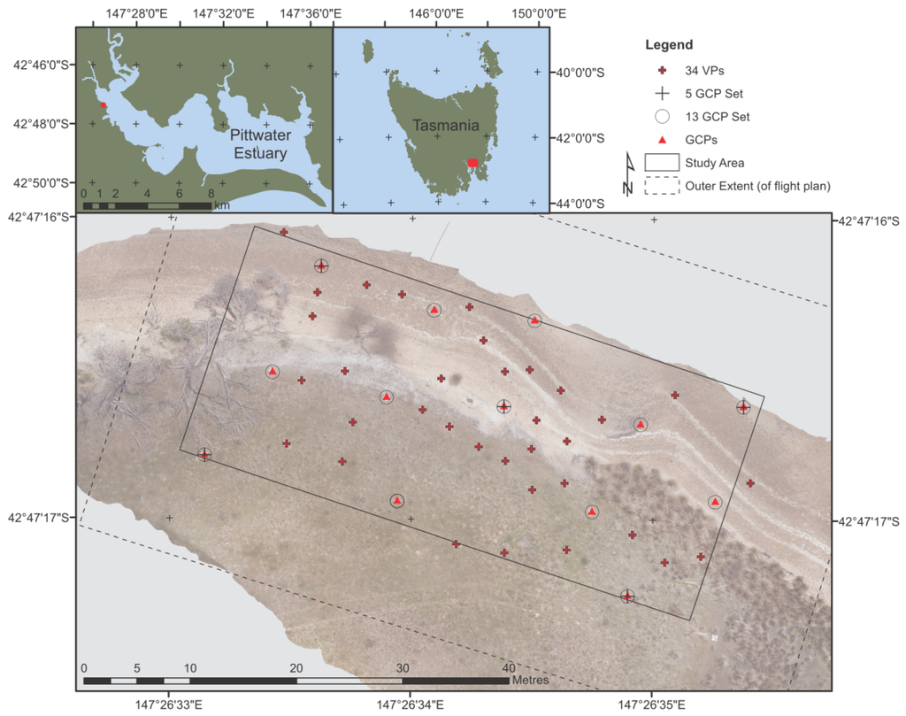
Figure 1. The study site is an eroding coastal scarp in a sheltered estuary in southeastern Tasmania, Australia. The map portrays the distribution of ground control and validation points.

Figure 1. The study site is an eroding coastal scarp in a sheltered estuary in southeastern Tasmania, Australia. The map portrays the distribution of ground control and validation points.

2.3. Ground Control and Validation Point Distribution

A total of 47 targets was distributed throughout the study area (Figure 1). Thirteen of these were used as GCPs and 34 as validation points (VPs). The GCPs were placed along two sides of the study area and through the middle. The targets were coded targets generated by Agisoft PhotoScan Professional (version 1.0.4) (Agisoft LLC) and printed onto 50 × 50 cm matte finish plastic boards with the black centre circle measuring 11 cm in diameter (Figure 2).

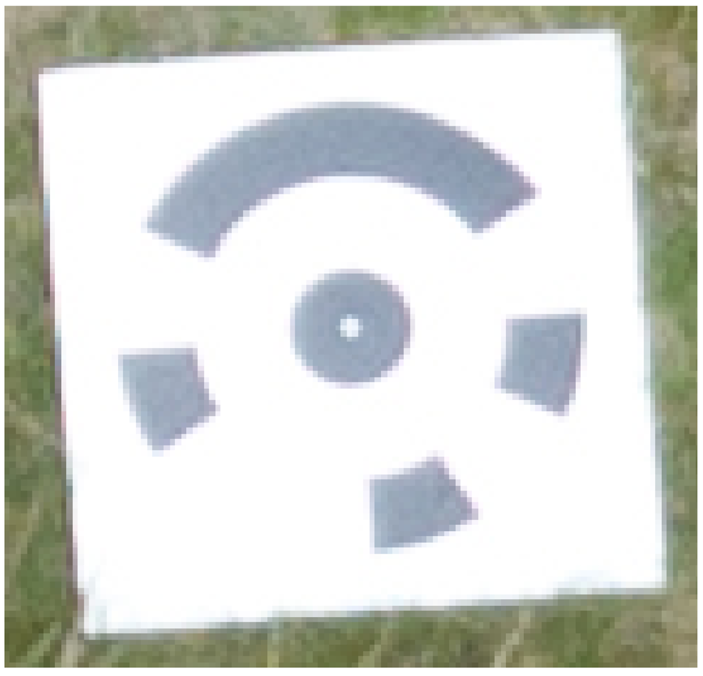
Figure 2. A printed PhotoScan coded target as imaged in one of the UAV photographs from the nadir image set.

Figure 2. A printed PhotoScan coded target as imaged in one of the UAV photographs from the nadir image set.

To provide for a pre-calibration, a target field adjacent to the study site was established. It comprised 47 printed PhotoScan targets distributed across an area of approximately 25 × 25 m. Ten targets were placed on top of tripods set up to provide as much variation in height as was practical and to provide a variation in height that was similar to that of the topography on the erosion site. The variation in target height was approximately 10% of the flying height (approximately 17–22 m AGL). In addition, two large measuring tapes were laid out in orthogonal directions to help with target matching and to provide an additional means of obtaining scale if necessary. Five GCPs, one in the centre of the target field and four approximately 5 m from the centre, were accurately surveyed using a total station; the remainder were left as uncoordinated tie points.

2.4. Precise Total Station Survey

The GCP and VPs were either theodolite stations or radiated detail points measured from those stations at least 3–4 times facing left and facing right. A short 30 cm prism pole with a staff bullseye bubble was used for all point radiations to reduce errors in vertical alignment of the prism over each point. The final coordinates were determined through a least squares network adjustment using LISCAD [35]. The precision achieved for GCP and VP points was ${\sigma }_X$ = 1 mm, ${\sigma }_Y$ = 1.4 mm and ${\sigma }_Z$ = 1.1 mm. A GCP and VP 3D precision of ${\sigma }_{XYZ}$ = 2 mm was adopted for subsequent calibration and model generation steps.

2.5. Degradation of Precise Total Station GCPs to Typical DGPS Accuracy

In most operational situations, a total station survey is too time consuming, and so, the DGPS survey is used to map GCPs. To compare the impact of surveying the GCPs using DGPS instead of a precise total station, the GCP coordinates were degraded using random values from a Gaussian distribution to introduce an error equivalent to typical DGPS. The accuracy setting was chosen based on descriptions in the manufacturer’s manual for a typical DGPS system (in this case, the Leica 1200 [36]). For surveys carried out in rapid static and static mode after initialization (compliance with ISO17123-8), RMS accuracy is quoted as 5 mm + 0.5 ppm horizontally and 10 mm + 0.5 ppm vertically. For surveys carried out in kinematic (phase) moving mode after initialization, RMS accuracy is quoted as 10 mm + 1 ppm horizontally and 20 mm + 1 ppm vertically. For this study site, the usual GPS base station location is approximately 2 km away, and assuming a lower accuracy in rapid static mode due to the possibility of systematic errors, the accuracy chosen to approximate a DGPS survey was the worst case RMS accuracy of a kinematic survey (20 mm + 1 ppm over 2 km = 22 mm). Each 3D coordinate for the GCPs (not the VPs) therefore had a random error applied constrained by the standard deviation: 1${\sigma }_{XYZ}$ = 22 mm. This was considered a more robust method of comparison than simply surveying the GCPs with DGPS, as the accuracy of the survey can be influenced by a range of factors, including satellite orbit geometry, obstructions, such as over-hanging trees or terrain, and error correlation between stations. Controlling the accuracy of these DGPS equivalent coordinates provides an indication of the impact of less precise GCPs, both on the calibration reliability and 3D reconstruction quality, although not addressing circumstances where the precision of the GPS coordinates is variable across the study site because of, for example, reduced satellite visibility.

2.6. UAV Survey

2.6.1. Flights for Pre-Calibration

To obtain convergent imagery of the 3D target field, a circular path was flown three times (Figure 3). For the first flight, the camera was mounted normally in landscape orientation. To ensure the targets were distributed throughout the frame of the camera, the camera mount roll angle was set so that the camera was in opposing portrait orientations in the second and third flights, respectively. The camera angle was set at 65° for each flight, and the UAV was flown in a circle (with an approximate radius of 6 m) at an altitude of approximately 18 m (AGL). The UAV was orientated to point at the centre GCP target in the calibration field to ensure convergent photography.

2.6.2. Study Site Flights

A traditional nadir photogrammetric flight path was flown over the main study site with 80%–90% overlap immediately after the calibration flights. The flight dynamics of the aircraft do not allow strict adherence to the flight plan; however, the aircraft usually stays within $\sim$2–3 m of the planned path. The AGL flying height was approximately 20–25 m, and the entire area was covered in two flights. Three additional flight lines were flown with the camera tilted so that a set of oblique images of the erosion could be captured. Again, these were flown so that overlap was approximately 80%–90%.

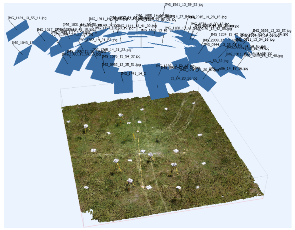
Figure 3. Calibration flight point cloud and camera network showing the 50 convergent camera stations and the 3D target array with some targets set up on tripods.

Figure 3. Calibration flight point cloud and camera network showing the 50 convergent camera stations and the 3D target array with some targets set up on tripods.

2.7. Scenarios

A total of 28 scenarios were tested. The assessed key variables were: (i) the camera calibration; (ii) the precision of GCPs; (iii) the number of GCPs; and (iv) the inclusion or exclusion of oblique photography. Table 1 lists those scenarios and assigns each scenario a code based on the variable settings of each.

Table 1. Scenarios tested and the codes assigned based on calibration type (checker board, target field, “on-the-job” self-calibration (OTJ self-cal.)), ground control point (GCP) σ, GCP count and whether the oblique imagery set was included.

Scenario Code	Calibration Type	Calibration Software	GCP σ	GCP Count	Oblique
			(mm)	<N>	(Yes/No)
Lens13GCP2mm	Checker board	Lens	2	13	No
Lens13GCP2mmObl	Checker board	Lens	2	13	Yes
PS13GCP2mm	Target field	PhotoScan	2	13	No
PS13GCP2mmObl	Target field	PhotoScan	2	13	Yes
Pre<N>GCP0mm (e.g., “Pre5GCP0mm”)	Target field	CalibCam	0	5,13	No
Pre<N>GCP0mmObl	Target field	CalibCam	0	5, 13	Yes
Pre<N>GCP2mm	Target field	CalibCam	2	5, 13	No
Pre<N>GCP2mmObl	Target field	CalibCam	2	5, 13	Yes
Pre<N>GCP22mm	Target field	CalibCam	22	5, 13	No
Pre<N>GCP22mmObl	Target field	CalibCam	22	5, 13	Yes
Self<N>GCP0mm	OTJ self-cal.	PhotoScan	0	5, 13	No
Self<N>GCP0mmObl	OTJ self-cal.	PhotoScan	0	5, 13	Yes
Self<N>GCP2mm	OTJ self-cal.	PhotoScan	2	5, 13	No
Self<N>GCP2mmObl	OTJ self-cal.	PhotoScan	2	5, 13	Yes
Self<N>GCP22mm	OTJ self-cal.	PhotoScan	22	5, 13	No
Self<N>GCP22mmObl	OTJ self-cal.	PhotoScan	22	5, 13	Yes

Table 1. Scenarios tested and the codes assigned based on calibration type (checker board, target field, “on-the-job” self-calibration (OTJ self-cal.)), ground control point (GCP) σ, GCP count and whether the oblique imagery set was included.

Scenario Code	Calibration Type	Calibration Software	GCP σ	GCP Count	Oblique
			(mm)	<N>	(Yes/No)
Lens13GCP2mm	Checker board	Lens	2	13	No
Lens13GCP2mmObl	Checker board	Lens	2	13	Yes
PS13GCP2mm	Target field	PhotoScan	2	13	No
PS13GCP2mmObl	Target field	PhotoScan	2	13	Yes
Pre<N>GCP0mm (e.g., “Pre5GCP0mm”)	Target field	CalibCam	0	5,13	No
Pre<N>GCP0mmObl	Target field	CalibCam	0	5, 13	Yes
Pre<N>GCP2mm	Target field	CalibCam	2	5, 13	No
Pre<N>GCP2mmObl	Target field	CalibCam	2	5, 13	Yes
Pre<N>GCP22mm	Target field	CalibCam	22	5, 13	No
Pre<N>GCP22mmObl	Target field	CalibCam	22	5, 13	Yes
Self<N>GCP0mm	OTJ self-cal.	PhotoScan	0	5, 13	No
Self<N>GCP0mmObl	OTJ self-cal.	PhotoScan	0	5, 13	Yes
Self<N>GCP2mm	OTJ self-cal.	PhotoScan	2	5, 13	No
Self<N>GCP2mmObl	OTJ self-cal.	PhotoScan	2	5, 13	Yes
Self<N>GCP22mm	OTJ self-cal.	PhotoScan	22	5, 13	No
Self<N>GCP22mmObl	OTJ self-cal.	PhotoScan	22	5, 13	Yes

2.8. Calibration Options

Four calibration options were evaluated:

(a)

a checker board pre-calibration using Lens [37];

(b)

a target field pre-calibration using PhotoScan [38];

(c)

a target field pre-calibration using CalibCam [39]; and

(d)

an “on-the-job” self-calibration using PhotoScan.

Each option is defined in Table 1 by the calibration type and the calibration software columns. These options were chosen based on the fact that PhotoScan is the main point cloud generation software package used in this research, and comparing it to a more traditional calibration package (CalibCam) and an automated calibration package (Lens) will allow us to understand the impact of the calibration method on generated point cloud accuracy. Option (a) (Lens) did not require any manual input, whereas the other three options required target centroiding in the imagery. Each calibration results in estimates of focal length, principal point coordinates, three radial distortion coefficients and two asymmetric lens distortion coefficients (following Brown [40]). Some conventions regarding calibration parameters in CalibCam differ slightly from those used in Lens and PhotoScan, such as different sign conventions, and these were modified accordingly.

2.8.1. Checker Board Pre-Calibration Using Lens

A set of photographs of a checker board pattern on a computer screen was taken from various angles whilst endeavouring to ensure that the pattern filled the field of view and remained in focus (which meant that the camera was not focussed at infinity). The image set was loaded into Lens. The software ran a bundle adjustment based on the matched corners of the checker board pattern to generate camera model parameters and lens distortion coefficients ready for import into PhotoScan. This process was repeated to ensure that the results were consistent. The residuals for one of the calibrations were marginally better, and the most accurate result was adopted.

2.8.2. Target Field Pre-Calibration Using PhotoScan

The set of 50 images from the convergent photography flights over the target field were loaded into PhotoScan, and the markers were detected. In PhotoScan, the marker detection algorithm is proprietary and requires considerable marker point placement verification and adjustment by the human operator. The marker centres were carefully checked and manually adjusted where required. Coordinates for the five GCP were uploaded and an initial alignment executed. The resulting point cloud was cleaned using PhotoScan’s “Gradual Selection” tool with the reprojection error filter. This tool allows points in the cloud to be selected and deleted based on a filter option, in this case a reprojection error value greater than approximately one (“Editing point cloud” in Agisoft PhotoScan [41]). After each deletion, the solution is optimised using PhotoScan’s “Optimize” tool that recalculates the bundle adjustment based on the new point set. The camera calibration coefficients derived via this alignment and self-calibration were exported for later application to the study site project.

Mismatches that occur during the initial alignment result in obviously incorrect points in the sparse point cloud, and leaving these incorrect points in the cloud will degrade the derived camera model. Editing the point cloud to clean it up so that the final optimised point cloud matches the surface as closely as possible is difficult, particularly when the mismatches occur over grassy terrain, as the “true” grass surface is not easily determined. Masking out all of the grass prior to alignment results in a very sparse point cloud, and in practice, it is not possible to reliably clean all erroneous grass points from the alignment-derived sparse point cloud. The first alignment can be cleaned and optimised to improve the derived camera model prior to point cloud densification; however, any remaining image matching errors will influence the derived camera model. The PhotoScan software allows precise placement of markers at the centre of targets in each image; however, it is not possible to align using only those defined target centres. Additionally, when the alignment completes, points corresponding to manually-placed target centres are not represented in the sparse point cloud. If there were a point corresponding to each ground control target, then it would be possible to delete all of the points, except those at marker locations, and to use PhotoScan to perform a more traditional calibration of the camera that bases the calibration only on the correspondence between target locations defined in the imagery and the marker location in the point cloud.

2.8.3. Target Field Pre-Calibration Using CalibCam

We employed another camera calibration software in this project, because of its additional functionality. CalibCam provides target centroiding tools, has the ability to fix calibration coefficients and allows the operator to set GCP XYZ standard deviation estimates and image space measurement accuracy estimates. Automatic and manual target centroid tools were used to place control markers on the 5 GCPs and the remaining uncoordinated targets (termed relative points in CalibCam) in all of the images. CalibCam target identification requires significant human input. The high resolution of the imagery coupled with the low flying height resulted in successful automatic identification of centroids for most GCP and VP targets; however, other targets closer to the edge of the images had significant view angles or were impacted by glare and were more difficult to centroid. Based on examination of the residuals and an assessment of the variance factor (0.9–1.1 is the target range) from the first resection (for interior orientation) and the bundle adjustment, 0.6 pixels were adopted as the image space measurement accuracy setting. The GCP standard deviation estimate was set as 2 mm for each X, Y and Z ordinate. The adjustment resulted in estimates of focal length, principal point coordinates, three radial distortion coefficients and two asymmetric distortion coefficients, and the result had a variance factor of 1.01 (with 1686 degrees of freedom).

2.8.4. “On-The-job” Self-Calibration Using Agisoft PhotoScan

The steps involved in generating a 3D point cloud together with the estimated position and pose of the camera stations and a solution for the camera model parameters are similar regardless of the SfM/MVS software used. For this study, the aim was to ensure that the scenarios were all based on the same PhotoScan project, so that there was minimal difference in the processing steps. This base project contained 172 good-quality, high-resolution images from the nadir and oblique flights that corresponded to 80%–90% overlap (any images that resulted in greater than 95% overlap were avoided). Any water or saturated (reflecting) sand was masked out of each image. The on-board navigation-grade GPS data were used to geocode the images, so that an initial alignment could be done based on these approximate positions. The 13 GCPs and 34 VPs were loaded into the project and detected in the imagery. Each marker was checked and edited when required to ensure that it was located and centroided in as many images as feasible. Once these markers were placed, the base project was used for the set up, and the following options were varied to produce 28 different operational scenarios:

(a)

The camera calibration settings were set to either the Lens, PhotoScan or CalibCam pre-calibration parameters and fixed or these parameters were left unfixed for the self-calibration scenarios;

(b)

Only the PhotoScan markers corresponding to the GCPs (5 or 13) were used for the final bundle adjustment, and no VPs nor camera positions were used in this step;

(c)

The marker coordinates were altered for the DGPS equivalent scenarios;

(d)

The estimated standard deviation for horizontal and vertical GCP accuracy (1${\sigma }_{XYZ}$) was set to either 0 mm, 2 mm or 22 mm and;

(e)

The oblique images were turned off for the scenarios with that image set excluded.

An alignment was run in each of the 28 projects. Each alignment resulted in a sparse point cloud, which was manually edited to remove any obvious erroneous points (typically where there was tall grass or complex woody vegetation). As described in (a), above, PhotoScan’s “Gradual Selection” and “Optimize” tools were used to clean the sparse cloud before generating a dense point cloud. The position and estimated error information were exported. Only the VP positions and their corresponding positions in the derived point clouds were used to calculate error metrics (RMSE, standard deviation, mean, median, maximum and minimum), and boxplots were generated to visualise these results.

2.9. GCP Accuracy (GCP σ)

The estimated accuracy of the total station survey was ${\sigma }_{XYZ}$ = 2 mm. PhotoScan only allows the input of a single estimate of “Marker Accuracy” (rather than an input for X, Y and Z accuracy for each GCP or the GCP set), and therefore, 2 mm was chosen as a reasonable approximation for the 3D GCP accuracy to one standard deviation (1σ). Based on this decision, it was necessary to set the same GCP accuracy value of 2 mm for each X, Y and Z ordinate in the CalibCam pre-calibration and a “Marker Accuracy” of 2 mm in the PhotoScan pre-calibration. In the PhotoScan documentation, it is suggested that “Marker Accuracy” should be set to zero “if the real marker accuracy is within 0.02 m” (Under Optimization at Agisoft PhotoScan WIKI [42]). In light of this recommendation, we included an additional scenario set with ${\sigma }_{XYZ}$ = 0 mm. The final standard deviation scenario set is based on the degraded GCP positions that mimic a DGPS survey (Section 2.5), with ${\sigma }_{XYZ}$ = 22 mm. Again, the accuracy settings were also set to 22 mm for the CalibCam (e.g., Pre13GCP22mmObl) and PhotoScan (e.g., PS13GCP22mmObl) pre-calibration scenarios (these have their calibrations fixed to the same coefficients as used in the 0 mm and 2 mm scenarios).

2.10. GCP Density (GCP Count)

As shown in Figure 1, two GCP sets were chosen. The first set can be considered a standard distribution of 13 GCPs, 9 around the periphery of the study area and 4 through the middle. The second set is an example of the sparsest GCP distribution that would be operationally acceptable, a GCP in each corner of the study area and one in the middle.

2.11. Inclusion/Exclusion of Oblique Photography

The whole study site was flown with nadir photography. Additional oblique photography was captured with a view toward improving the 3D reconstruction of the main erosion scarp (cracks, overhangs and small caves). For this study, the set of oblique photographs were taken at an AGL flying height of approximately 20–25 m with the camera angled between 45° and 65° oriented to face the erosion scarp. In the scenarios, these oblique images were included/excluded to assess their impact on the accuracy of the self-calibration and the derived model.

2.12. Accuracy Assessment Using Verification Points

The method used to assess the accuracy of the derived models in comparison to the total station survey is to report the difference between the precisely-surveyed VPs and their identified location in the derived point cloud. In PhotoScan, this is done by placing a non-ground control marker in the centre of the target in multiple images, and PhotoScan reports the difference between the estimated position of those image marker points in the model to the supplied precise survey coordinate (as X, Y and Z error). In each GCP density scenario, only the chosen set of GCPs were activated as ground control. The remaining GCPs were ignored in these scenarios. In each GCP accuracy scenario, the GCP coordinates provided were either the set of precise survey coordinates or the DGPS equivalents. For each scenario, a set of VP errors were exported and used to derive metrics for assessing accuracy in X, Y, Z, XY and XYZ (RMSE, mean, median, standard deviation, minimum and maximum).

3. Results and Discussion

The mapping accuracy achieved for each of the scenarios is summarised in the following figures and tables. Refer to Table 1 for a summary of the coded scenarios.

3.1. Calibration Options

Pre-calibration based on a target field (PS13GCP2mm/PS13GCP2mmObl and Pre13GCP2mm/ Pre13GCP2mmObl), on-the-job self-calibration (Self13GCP2mm/Self13GCP2mmObl) and pre-calibration derived from a checker board pattern (Lens13GCP2mm and Lens13GCP2mmObl) are compared in Figure 4 and Table 2. The results indicate that the checker board calibration performed the most poorly. This is particularly evident in the vertical accuracy statistics, with substantially lower precision and significant bias. Pre-calibration solutions perform marginally worse than on-the-job self-calibration solutions, particularly in terms of vertical accuracy. The control in these scenarios is very precise, and with the exception of models that employ the checker board pre-calibration (Lens13GCP2mm/Lens13GCP2mmObl), this leads to precise models with no evidence of significant systematic errors. An on-the-job self-calibration that includes oblique photography (Self13GCP2mmObl) results in the most accurate model. That accuracy degrades when the oblique imagery is not included in the solution and results in a model with accuracy comparable to the robust pre-calibration. Measured in terms of achieved precision, the ranking of choices is:

• On-the-job calibration using a network that includes oblique photography.
• Either an on-the-job calibration using only nadir photography or a robust pre-calibration.

Figure 4. Box plots of the four calibration options for σ = 2 mm and with and without oblique imagery.

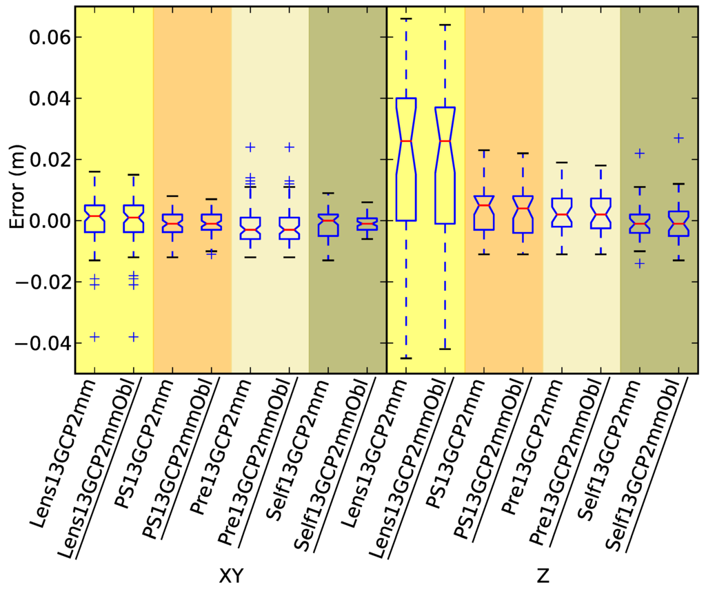
Figure 4. Box plots of the four calibration options for σ = 2 mm and with and without oblique imagery.

3.2. GCP Accuracy (GCP σ)

In assessing the impact of GCP accuracy, we will first consider the 13 GCP scenarios (Figure 5) before comparing and examining the impact of reducing the number of GCPs to five in Section 3.3 (Figure 6). The resulting RMSEs are summarized in Table 3.

Table 2. RMSE for each of the four calibration options tested for σ = 2 mm and with and without oblique imagery.

Scenario	RMSE${}_{\mathrm{XY}}$	RMSE${}_Z$
	(mm)	(mm)
Lens13GCP2mm	8.8	41.0
Lens13GCP2mmObl	8.7	39.3
PS13GCP2mm	4.2	8.3
PS13GCP2mmObl	4.1	8.1
Pre13GCP2mm	7.3	7.1
Pre13GCP2mmObl	7.1	7.2
Self13GCP2mm	5.1	6.4
Self13GCP2mmObl	3.2	7.8

Table 2. RMSE for each of the four calibration options tested for σ = 2 mm and with and without oblique imagery.

Scenario	RMSE${}_{\mathrm{XY}}$	RMSE${}_Z$
	(mm)	(mm)
Lens13GCP2mm	8.8	41.0
Lens13GCP2mmObl	8.7	39.3
PS13GCP2mm	4.2	8.3
PS13GCP2mmObl	4.1	8.1
Pre13GCP2mm	7.3	7.1
Pre13GCP2mmObl	7.1	7.2
Self13GCP2mm	5.1	6.4
Self13GCP2mmObl	3.2	7.8

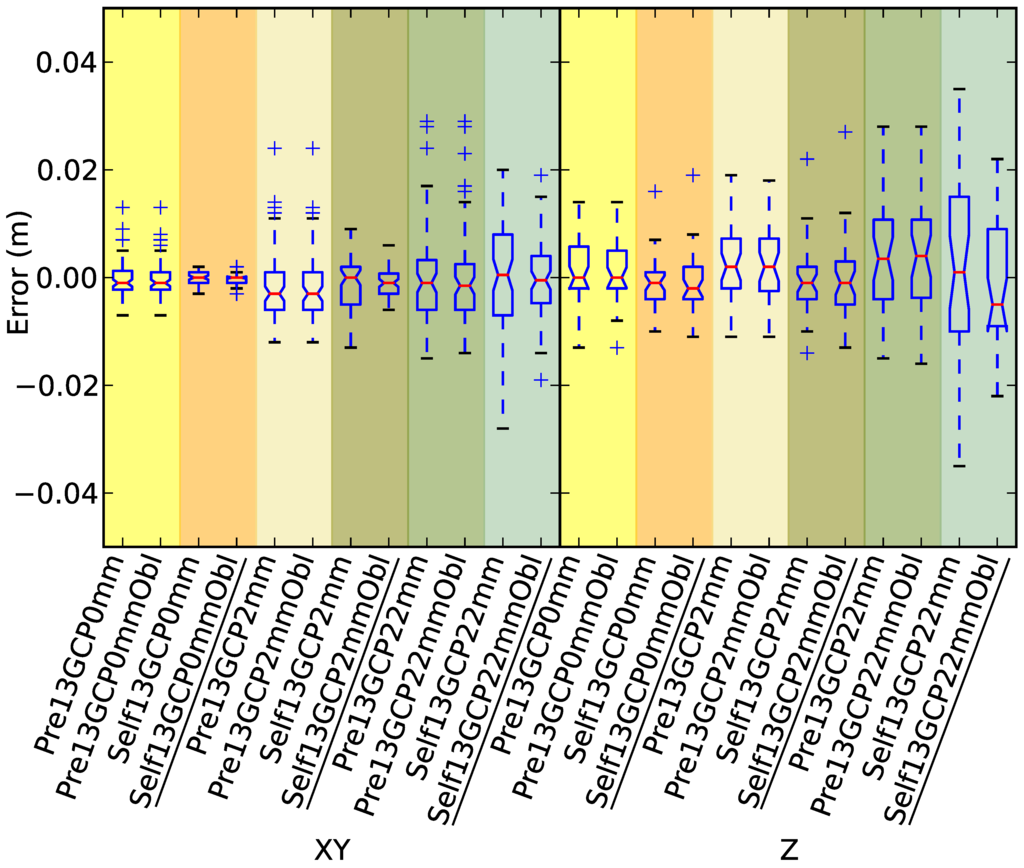
Figure 5. Pre-calibration versus on-the-job self-calibration scenario comparison using a strong control network (13 GCPs), with and without oblique imagery.

Figure 5. Pre-calibration versus on-the-job self-calibration scenario comparison using a strong control network (13 GCPs), with and without oblique imagery.

Figure 6. Pre-calibration versus on-the-job self-calibration scenario comparison using a sparse control network (five GCPs), with and without oblique imagery.

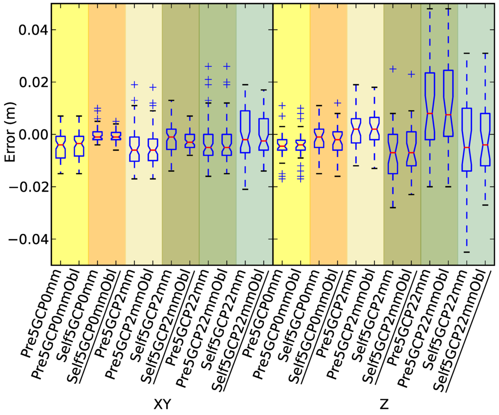
Figure 6. Pre-calibration versus on-the-job self-calibration scenario comparison using a sparse control network (five GCPs), with and without oblique imagery.

Table 3. RMSE for pre-calibration and on-the-job self-calibration for three different GCP σ scenarios when using a strong control network (13 GCPs) and a sparse control network (5 GCPs).

Scenario	RMSE${}_{\mathrm{XY}}$	RMSE${}_Z$	Scenario	RMSE${}_{\mathrm{XY}}$	RMSE${}_Z$
	(mm)			(mm)	(mm)
Pre13GCP0mm	3.6	5.8	Self13GCP0mm	1.4	5.1
Pre13GCP0mmObl	3.5	5.8	Self13GCP0mmObl	1.3	5.9
Pre5GCP0mm	7.0	7.3	Self5GCP0mm	2.7	5.8
Pre5GCP0mmObl	6.7	7.1	Self5GCP0mmObl	2.1	6.3
Pre13GCP2mm	7.3	7.1	Self13GCP2mm	5.1	6.4
Pre13GCP2mmObl	7.1	7.2	Self13GCP2mmObl	3.2	7.8
Pre5GCP2mm	7.1	7.4	Self5GCP2mm	6.0	13.6
Pre5GCP2mmObl	8.8	7.8	Self5GCP2mmObl	4.3	11.5
Pre13GCP22mm	9.1	12.4	Self13GCP22mm	10.3	16.6
Pre13GCP22mmObl	9.1	12.6	Self13GCP22mmObl	7.0	11.9
Pre5GCP22mm	8.7	20.0	Self5GCP22mm	10.5	19.8
Pre5GCP22mmObl	8.6	20.0	Self5GCP22mmObl	7.3	15.9

Table 3. RMSE for pre-calibration and on-the-job self-calibration for three different GCP σ scenarios when using a strong control network (13 GCPs) and a sparse control network (5 GCPs).

Scenario	RMSE${}_{\mathrm{XY}}$	RMSE${}_Z$	Scenario	RMSE${}_{\mathrm{XY}}$	RMSE${}_Z$
	(mm)			(mm)	(mm)
Pre13GCP0mm	3.6	5.8	Self13GCP0mm	1.4	5.1
Pre13GCP0mmObl	3.5	5.8	Self13GCP0mmObl	1.3	5.9
Pre5GCP0mm	7.0	7.3	Self5GCP0mm	2.7	5.8
Pre5GCP0mmObl	6.7	7.1	Self5GCP0mmObl	2.1	6.3
Pre13GCP2mm	7.3	7.1	Self13GCP2mm	5.1	6.4
Pre13GCP2mmObl	7.1	7.2	Self13GCP2mmObl	3.2	7.8
Pre5GCP2mm	7.1	7.4	Self5GCP2mm	6.0	13.6
Pre5GCP2mmObl	8.8	7.8	Self5GCP2mmObl	4.3	11.5
Pre13GCP22mm	9.1	12.4	Self13GCP22mm	10.3	16.6
Pre13GCP22mmObl	9.1	12.6	Self13GCP22mmObl	7.0	11.9
Pre5GCP22mm	8.7	20.0	Self5GCP22mm	10.5	19.8
Pre5GCP22mmObl	8.6	20.0	Self5GCP22mmObl	7.3	15.9

Similar to the findings reported in Section 3.1, when control is precise ($\sigma \le$ 2 mm), then on-the-job self-calibration (Self13GCP0mm/Self13GCP0mmObl and Self13GCP2mm/Self13GCP2mmObl) and pre-calibration (Pre13GCP0mm/Pre13GCP0mmObl and Pre13GCP2mm/Pre13GCP2mmObl) both produced very accurate models, and including oblique imagery did not significantly impact the results. Fixing the marker accuracy setting in PhotoScan at 0 mm produced more accurate models than those that used the 2 mm setting, particularly for the on-the-job self-calibration scenarios.

When GCP precision was degraded to 22 mm, the positive impact of including oblique imagery became more apparent in the self-calibration scenario (Self13GCP22mmObl), which was shown to be the most accurate 22 mm scenario. The pre-calibration RMSE${}_{XY}$ = 9.1 mm, and on-the-job self-calibration RMSE${}_{XY}$ = 7.0 mm. There was a 3.3 mm horizontal and 4.7 mm vertical improvement for the on-the-job self-calibration scenario with oblique imagery (Self13GCP22mmObl) versus the on-the-job self-calibration scenario without oblique imagery (Self13GCP22mm). The implication is that if the GCP survey is undertaken using DGPS (σ = 22 mm), then on-the-job self-calibration with oblique imagery produces the most accurate model.

3.3. GCP Density (GCP Count)

The impact on model accuracy of reducing the number of GCPs to five will be assessed (Figure 6), and then the 13 GCP (dense) and five GCP (sparse) scenarios will be compared (Figure 5 versus Figure 6). Table 3 summarises these results.

When the GCP density was sparse (five GCPs), the overall accuracy was degraded, particularly in the vertical, regardless of calibration choice. When control was precise ($\sigma \le$ 2 mm), the bias in the pre-calibration solutions (particularly in XY) implies that on-the-job self-calibration produced the most accurate models, and including oblique imagery had little impact. When control was less accurate (σ = 22 mm), all solutions show bias, and on-the-job self-calibration with oblique imagery produced the most accurate model (particularly when comparing vertical accuracy). Once again, on-the-job self-calibration with oblique imagery was the best option when σ = 22 mm and when control was sparse. As in the dense control scenarios, including oblique imagery provided little or no benefit when the control was precisely surveyed.

When comparing dense (13 GCPs) and sparse (five GCPs) GCP density scenarios, the most accurate models were produced when using a higher number of GCPs. The impact was smaller when control was precise, particularly when using pre-calibration. The vertical accuracy was more greatly influenced than the horizontal accuracy when the number of GCPs was degraded, particularly when σ = 22 mm and when σ = 2 mm. When there were only five GCPs, fixing the control (setting σ = 0 mm) had a significant impact on accuracy in the on-the-job self-calibration case, particularly in the vertical. The same impact was not seen in the 13 GCP scenarios. When GCPs were less accurate (σ = 22 mm), the addition of oblique imagery improved model accuracy in both the 13 and five GCP cases. Reducing the number of GCPs degraded the vertical accuracy of the models, whereas the horizontal accuracy of the models was not adversely impacted by this reduction in GCP density. In this study, five GCPs represents a practical minimum, since fewer would result in significant areas of terrain without nearby ground control, and 13 is likely to be a practical maximum, since residuals are approaching the limits of measurement precision. The findings of this study do suggest that there is scope for undertaking a similar study over a larger area in order to produce more ‘scalable’ rules for camera calibration and GCP distribution.

The overarching goal of this research is to better understand the implications of UAV survey design on the capacity to reliably measure topographic change, such as occurs in eroding coastal landscapes.

The precise survey used to validate our model demonstrates that UAV-MVS has provided sub-centimetre accuracy point clouds from 25–30 m AGL, which, in turn, allows change detection at the centimetre level.

The investigation demonstrates that self-calibration is comparable to pre-calibration when the GCP survey is designed with careful consideration of GCP survey accuracy, distribution and density, coupled with a well-designed camera network. Including oblique imagery may improve the accuracy of the results, and for change detection studies, these oblique images better ensure that terrain complexity is mapped.

A future study will investigate further the spatial distribution of errors. In this study, no doming, such as reported by James and Quinton [28], Javernick et al. [43], Woodget et al. [44], was evident in either the sparse or the dense GCP density scenarios.

This study helps to inform operational decisions in the survey design process and to provide insight into the impact of calibration choices, oblique imagery inclusion, ground control accuracy and ground control density on the accuracy of the resultant photogrammetric model.

4. Conclusions

The use of UAV-MVS surveys to generate 3D point clouds for coastal erosion monitoring requires careful survey design to ensure sufficient accuracy for change detection. The influence of calibration methodology, ground control point accuracy, the number of ground control points (GCPs) and the inclusion of oblique imagery was investigated. Accuracy was assessed by comparing precisely-surveyed verification points with their photogrammetrically-derived coordinates. This study is the first to undertake a precise total station field survey with $\sigma \le$ 2 mm for the purposes of assessing the impact of these survey design choices on UAV-MVS 3D models of natural terrain.

Under a range of typical operating scenarios, four calibration options were assessed: on-screen checker board pre-calibration; a pre-calibration using Agisoft PhotoScan; a pre-calibration using 3DM CalibCam; and a self-calibration using Agisoft PhotoScan. The on-screen checker board pre-calibration was shown to be the least accurate method (vertical RMSE was $\sim$5 times less accurate than the other methods), and so, the conclusions here summarise the findings for flown CalibCam pre-calibrations and PhotoScan on-the-job self-calibrations. The results indicate that when a dense array of precise ground control and no oblique imagery was employed in the solutions, then the differences between a pre-calibration and an on-the-job self-calibration were not substantial (on-the-job self-calibration was marginally more accurate: the horizontal root mean square error (RMSE) differed by $\sim$2 mm (RMSE${}_{XY}$ for pre-calibration was 7.3 mm compared to 5.1 mm for self-calibration); the vertical RMSE differed by 0.7 mm (RMSE${}_Z$ was 7.1 mm compared to 6.4 mm). When oblique imagery was incorporated into the same solutions, self-calibration remained the more accurate solution for horizontal coordinates (with the difference increasing to 3.9 mm, RMSE${}_{XY}$ was 3.2 mm, whereas pre-calibration RMSE${}_{XY}$ was 7.1 mm) and still comparable for vertical accuracy (although in this case, 0.6 mm less accurate than the pre-calibration).

The results indicate that when the number of ground control points was reduced (to only five GCPs with $\sigma \le$ 2 mm), the accuracy of the solutions degraded, but more so for the self-calibration solution. However, our results suggest that this degradation of the self-calibration can be mitigated by increasing the accuracy of the ground control. These results indicate that when the ground control accuracy is high, the addition of oblique imagery has little impact on model accuracy.

When the dense array of ground control was geolocated at more common operational survey accuracy (σ = 22 mm) for both the pre-calibration and on-the-job self-calibration scenarios, then our results show that, with the inclusion of oblique imagery, the self-calibration performed better than a pre-calibration. In this scenario, horizontal accuracy degraded by only 2.0 mm for pre-calibration (RMSE${}_{XY}$ went from 7.1–9.1 mm) compared to 3.8 mm for on-the-job self-calibration (RMSE${}_{XY}$ went from 3.2–7.0 mm). When comparing on-the-job self-calibration scenarios, then our results show that a solution without oblique photography performed more poorly than one with oblique photography (horizontal accuracy reduced by 3.3 mm (RMSE${}_{XY}$ went from 10.3–7.0 mm) and vertical accuracy reduced by 4.7 mm (RMSE${}_Z$ went from 16.6–11.9 mm)). When the sparse array, instead of the dense array, of ground control was geolocated at more common operational survey accuracy (σ = 22 mm) for both the pre-calibration and on-the-job self-calibration scenarios, including oblique imagery significantly improved the on-the-job self-calibration results (in our case, by 3.2 mm horizontally (RMSE${}_{XY}$ went from 10.5–7.3 mm) and 3.9 mm vertically (RMSE${}_Z$ went from 19.8–15.9 mm)).

Regardless of GCP accuracy, pre-calibration may be operationally expensive, and so, the better option is then to employ on-the-job self-calibration ensuring that there is sufficient overlap and that the imagery extends beyond the focus area. Including oblique imagery is therefore advised. The GCPs should be distributed across the area to be mapped, particularly around the periphery. The GCP density should be high enough that it will overcome the issues seen in the sparse control scenarios, such as the degradation in overall accuracy. Vertical accuracy is particularly susceptible to poor GCP distribution and density. Questions related to accuracy prediction, configuration considerations, such as GCP distribution, and variations in camera network design will be the focus of a future study. Finally, it is important to understand that the inclusion or exclusion of oblique imagery in the scenarios was focussed on the impact on horizontal and vertical accuracy and does not take into account the improvements to the 3D model that are seen when adding oblique imagery to the camera station network. The influence of oblique imagery on the quality of the 3D model will be investigated in future research.

References

- Snavely, N.; Seitz, S.M.; Szeliski, R. Modeling the world from internet photo collections. Int. J. Comput. Vis. 2007, 80, 189–210. [Google Scholar] [CrossRef]
- Snavely, N. Bundler: Structure from Motion (SfM) for Unordered Image Collections. Available online: http://www.cs.cornell.edu/snavely/bundler/ (accessed on 27 January 2011).
- Lowe, D.G. Distinctive image features from scale-invariant keypoints. Int. J. Comput. Vision 2004, 60, 91–110. [Google Scholar] [CrossRef]
- Furukawa, Y.; Ponce, J. Accurate, dense, and robust multi-view stereopsis. IEEE Trans. Pattern Anal. Mach. Intell. 2009, 32, 1362–1376. [Google Scholar] [CrossRef] [PubMed]
- Liu, H. Algorithmic foundation and software tools for extracting shoreline features from remote sensing imagery and LiDAR data. J. Geogr. Inf. Syst. 2011, 3, 99–119. [Google Scholar] [CrossRef]
- Verhoeven, G.; Taelman, D.; Vermeulen, F. Computer vision-based orthophoto mapping of complex archaeological sites: The ancient quarry of itaranha (Portugal-Spain). Archaeometry 2012, 54, 1114–1129. [Google Scholar] [CrossRef]
- Vu, H.H.; Labatut, P.; Pons, J.P.; Keriven, R. High accuracy and visibility-consistent dense multiview stereo. IEEE Trans. Geosci. Remote 2012, 34, 889–901. [Google Scholar] [CrossRef] [PubMed]
- Turner, D.; Lucieer, A.; Wallace, L. Direct georeferencing of ultrahigh-resolution UAV imagery. IEEE Trans. Geosci. Remote 2014, 52, 2738–2745. [Google Scholar] [CrossRef]
- Turner, D.; Lucieer, A.; Watson, C. An automated technique for generating georectified mosaics from ultra-high resolution Unmanned Aerial Vehicle (UAV) imagery, based on Structure from Motion (SfM) point clouds. Remote Sens. 2012, 4, 1392–1410. [Google Scholar] [CrossRef]
- Lucieer, A.; De Jong, S.; Turner, D. Mapping landslide displacements using Structure from Motion (SfM) and image correlation of multi-temporal UAV photography. Prog. Phys. Geog. 2013, 38, 97–116. [Google Scholar] [CrossRef]
- Lucieer, A.; Robinson, S.; Turner, D. Unmanned aerial vehicle (UAV) remote sensing for hyperspatial terrain mapping of Antarctic moss beds based on Structure from Motion (SfM) point clouds. In Proceedings of the 34th International Symposium on Remote Sensing of Environment, Sydney, NSW, Australia, 10–15 April 2011.
- Harwin, S.; Lucieer, A. Assessing the accuracy of georeferenced point clouds produced via multi-view stereopsis from Unmanned Aerial Vehicle (UAV) imagery. Remote Sens. 2012, 4, 1573–1599. [Google Scholar] [CrossRef]
- Prahalad, V.; Sharples, C.; Kirkpatrick, J.; Mount, R. Is wind-wave fetch exposure related to soft shoreline change in swell-sheltered situations with low terrestrial sediment input? J. Coast. Conserv. 2015, 19, 23–33. [Google Scholar] [CrossRef]
- Tahar, K.N.; Ahmad, A. UAV-based stereo vision for photogrammetric survey in aerial terrain mapping. In Proceedings of the 2011 IEEE International Conference on Computer Applications and Industrial Electronics (ICCAIE), Penang, Malaysia, 4–7 December 2011; pp. 443–447.
- Neitzel, F.; Klonowski, J. Mobile 3D mapping with a low-cost UAV system. ISPRS Arch. 2011, 38, 1–6. [Google Scholar] [CrossRef]
- Rosnell, T.; Honkavaara, E. Point cloud generation from aerial image data acquired by a quadrocopter type micro unmanned aerial vehicle and a digital still camera. Sensors 2012, 12, 453–480. [Google Scholar] [CrossRef] [PubMed]
- Carvajal, F.; Agüera, F.; Pérez, M. Surveying a landslide in a road embankment using Unmanned Aerial Vehicle photogrammetry. ISPRS Arch. 2011, 38, 1–6. [Google Scholar] [CrossRef]
- Mancini, F.; Dubbini, M.; Gattelli, M.; Stecchi, F.; Fabbri, S.; Gabbianelli, G. Using Unmanned Aerial Vehicles (UAV) for high-resolution reconstruction of topography: The structure from motion approach on coastal environments. Remote Sens. 2013, 5, 6880–6898. [Google Scholar] [CrossRef]
- Strecha, C.; von Hansen, C.; Gool, L.V.; Fua, P.; Thoennessen., U. On benchmarking camera calibration and multi-view stereo for high resolution imagery. In Proceedings of the 2008 IEEE Conference on Computer Vision and Pattern Recognition (CVPR), Anchorage, AK, USA, 24–26 June 2008.
- Vallet, J.; Panissod, F.; Strecha, C.; Tracol, M. Photogrammetric performance of an ultra light weight swinglet “UAV”. ISPRS Arch. 2011, 38, 253–258. [Google Scholar] [CrossRef]
- James, M.; Robson, S. Straightforward reconstruction of 3D surfaces and topography with a camera: Accuracy and geoscience application. J. Geophys. Res. 2012, 117, 1–17. [Google Scholar] [CrossRef]
- Flener, C.; Vaaja, M.; Jaakkola, A.; Krooks, A.; Kaartinen, H.; Kukko, A.; Kasvi, E.; Hyyppä, H.; Hyyppä, J.; Alho, P. Seamless mapping of river channels at high resolution using mobile LiDAR and UAV-Photography. Remote Sens. 2013, 5, 6382–6407. [Google Scholar] [CrossRef]
- Westoby, M.; Brasington, J.; Glasser, N.; Hambrey, M.; Reynolds, J. Structure-from-Motion photogrammetry: A low-cost, effective tool for geoscience applications. Geomorphology 2012, 179, 300–314. [Google Scholar] [CrossRef]
- D’Oleire-Oltmanns, S.; Marzolff, I.; Peter, K.; Ries, J. Unmanned Aerial Vehicle (UAV) for monitoring soil erosion in Morocco. Remote Sens. 2012, 4, 3390–3416. [Google Scholar] [CrossRef]
- Fraser, C. Automatic camera calibration in close range photogrammetry. Photogramm. Eng. Remote Sens. 2013, 79, 381–388. [Google Scholar] [CrossRef]
- Fraser, C.S.; Ganci, G.; Shortis, M. Multi-sensor system self-calibration. Int. Soc. Opt. Eng. 1995. [Google Scholar] [CrossRef]
- Remondino, F.; Fraser, C.S. Digital camera calibration methods: Considerations and comparisons. In Proceedings of the 2006 ISPRS Commission V Symposium “Image Engineering and Vision Metrology”, Dresden, Germany, 25–27 September 2006.
- James, M.; Quinton, J.N. Ultra-rapid topographic surveying for complex environments: The hand-held mobile laser scanner (HMLS). Earth Surf. Proc. Land. 2014, 39, 138–142. [Google Scholar] [CrossRef]
- Granshaw, S.I. Bundle adjustment methods in engineering photogrammetry. Photogramm. Rec. 1980, 10, 181–207. [Google Scholar] [CrossRef]
- James, M.R.; Robson, S. Mitigating systematic error in topographic models derived from UAV and ground-based image networks. Earth Surf. Proc. Land. 2014, 39, 1413–1420. [Google Scholar] [CrossRef]
- Fryer, J. Camera calibration. In Close Range Photogrammetry and Machine Vision; Atkinson, K., Ed.; Whittles Publishing: Caithness, UK, 1996; pp. 156–179. [Google Scholar]
- Wackrow, R.; Chandler, J.; Gardner, T. Minimising systematic errors in DEMs caused by an inaccurate lens model. ISPRS Arch. 2008, 37, 1–6. [Google Scholar]
- Wackrow, R.; Chandler, J.H. Minimising systematic error surfaces in digital elevation models using oblique convergent imagery. Photogramm. Rec. 2011, 26, 16–31. [Google Scholar] [CrossRef]
- Mikrokopter. MikroKopter WIKI. Available online: http://www.mikrokopter.com (accessed on 7 February 2012).
- LISTECH LISCAD; Version 10.1; LISTECH Pty Ltd: Richmond, Victoria, Australia, 2013.
- Leica Geosystems. Leica GPS1200 Brochure. Available online: http://www.leica-geosystems.com/downloads123/zz/gps/general/brochures-datasheet/GPS1200_TechnicalData_en.pdf (accessed on 11 September 2014).
- Agisoft Lens; Version 040.1.1718 beta 64 bit; AgiSoft LLC: Petersburg, Russia, 2014.
- Agisoft PhotoScan; Professional Edition Version 1.0.4.1847 64 bit; AgiSoft LLC: Petersburg, Russia, 2014.
- 3DM CalibCam; Version 2.2a; ADAM Technology: Perth, Australia, 2006.
- Brown, D. Close-range camera calibration. Photogramm. Eng. Remote Sens. 1971, 37, 855–866. [Google Scholar]
- Agisoft PhotoScan. In User Manual: Professional Edition Version 1.0.4.1847 64 bit; AgiSoft LLC: Petersburg, Russia, 2014.
- Agisoft PhotoScan WIKI. Agisoft PhotoScan WIKI. Available online: http://www.agisoft.ru/wiki/PhotoScan/Tips_and_Tricks (accessed on 13 June 2014).
- Javernick, L.; Brasington, J.; Caruso, B. Modeling the topography of shallow braided rivers using Structure-from-Motion photogrammetry. Geomorphology 2014, 213, 166–182. [Google Scholar] [CrossRef]
- Woodget, A.S.; Carbonneau, P.E.; Visser, F.; Maddock, I.P. Quantifying submerged fluvial topography using hyperspatial resolution UAS imagery and structure from motion photogrammetry. Earth Surf. Proc. Land. 2015, 40, 47–64. [Google Scholar] [CrossRef]
© 2015 by the authors; licensee MDPI, Basel, Switzerland. This article is an open access article distributed under the terms and conditions of the Creative Commons Attribution license (http://creativecommons.org/licenses/by/4.0/).