Comparison of NDVIs from GOCI and MODIS Data towards Improved Assessment of Crop Temporal Dynamics in the Case of Paddy Rice

Abstract

The monitoring of crop development can benefit from the increased frequency of observation provided by modern geostationary satellites. This paper describes a four-year testing period from 2010 to 2014, during which satellite images from the world's first Geostationary Ocean Color Imager (GOCI) were used for spectral analyses of paddy rice in South Korea. A vegetation index was calculated from GOCI data based on the bidirectional reflectance distribution function (BRDF)-adjusted reflectance, which was then used to visually analyze the seasonal crop dynamics. These vegetation indices were then compared with those calculated using the Moderate-resolution Imaging Spectroradiometer (MODIS)-normalized difference vegetation index (NDVI) based on Nadir BRDF-adjusted reflectance. The results show clear advantages of GOCI, which provided four times better temporal resolution than the combined MODIS sensors, interpreting subtle characteristics of the vegetation development. Particularly in the rainy season, when data acquisition under clear weather conditions was very limited, it was possible to find cloudless pixels within the study sites by compiling GOCI images obtained from eight acquisition periods per day, from which the vegetation index could be calculated. In this study, ground spectral measurements from CROPSCAN were also compared with satellite-based vegetation products, despite their different index magnitude, according to systematic discrepancy, showing a similar crop development pattern to the GOCI products. Consequently, we conclude that the very high temporal resolution of GOCI is very beneficial for monitoring crop development, and has potential for providing improved information on phenology.

1. Introduction

Phenological changes in land surface vegetation, which are closely related to boundary-layer atmospheric dynamics, have been increasingly seen as important signals of year-to-year climate variations or even global environmental changes [1,2,3,4]. The time series of wide-field-of-view sensors such as the Advanced Very High Resolution Radiometer (AVHRR), Medium Resolution Imaging Spectrometer (MERIS), Moderate-resolution Imaging Spectroradiometer (MODIS), and SPOT VEGETATION have proven appropriate for phenology detection from multi-temporal vegetation indices [5,6,7,8,9,10]. Particularly for crop monitoring, the MODIS multi-year time-series analysis may make a significant contribution to providing temporal dynamics on rice cropping systems, as well as determining the spatial distribution of rice phenology [11,12,13,14]. Furthermore, the temporal information of crops from low resolution satellite imagery is useful for mapping different vegetation and crop types [15], and assessing yield and production [16].

When observing reflected solar spectral radiation from vegetation on the land surface using an optical sensor, cloud cover can prevent the accurate collection of surface physical characteristics. It is impossible to obtain surface spectral information from optical satellites over a cloudy area because the wavelength of the reflected solar spectrum cannot penetrate the cloudy area. Therefore, it is important to secure timely surface information from optical sensors under severe weather conditions. To overcome the limitations of polar orbiting reflective wavelength sensors for interpreting vegetation development, various temporal smoothing techniques such as Fourier harmonics, threshold methods, and curve-fitting methods have been suggested to fill or smooth noise and sparse greenness observations from satellite images [17,18,19,20,21,22,23,24]. Although these techniques are effective for dealing with sporadic missing data, using them for long-term missing data during the cloudy monsoon period of crop growth may produce detrimental results. Therefore, it is important to use high-temporal-resolution satellite images to obtain meaningful information. The combined MODIS observation characteristics from the Terra and Aqua satellites have been optimized to estimate vegetation phenology under normal weather conditions. However, during the monsoon rainy season (called Jang-Ma in Korea) between June and August, the high level of cloud cover makes it difficult to acquire timely surface information from MODIS observations.

The objective of this study was to calculate vegetation index profiles for two points using data from the first Korean geostationary orbit satellite, the Geostationary Ocean Color Imager (GOCI) launched successfully on 27 June 2010. GOCI was designed to detect, monitor, and predict regional ocean phenomena around Korea but is equipped with eight spectral bands (six visible, two near infrared). So, there is great interest in its terrestrial application because of its high temporal resolution as well as its vegetation-sensitive multispectral bands. The high temporal resolution of GOCI allows for eight acquisitions of imagery during the daytime and it is four times better than the MODIS observation system combining Terra and Aqua. The frequent observation characteristics of GOCI are therefore expected to provide more reliable information on crop temporal dynamics. We compared for two sample sites four-year GOCI data with corresponding MODIS image data to detect spectral signals according to crop growth and development.

2. Materials and Methods

2.1. Study Area

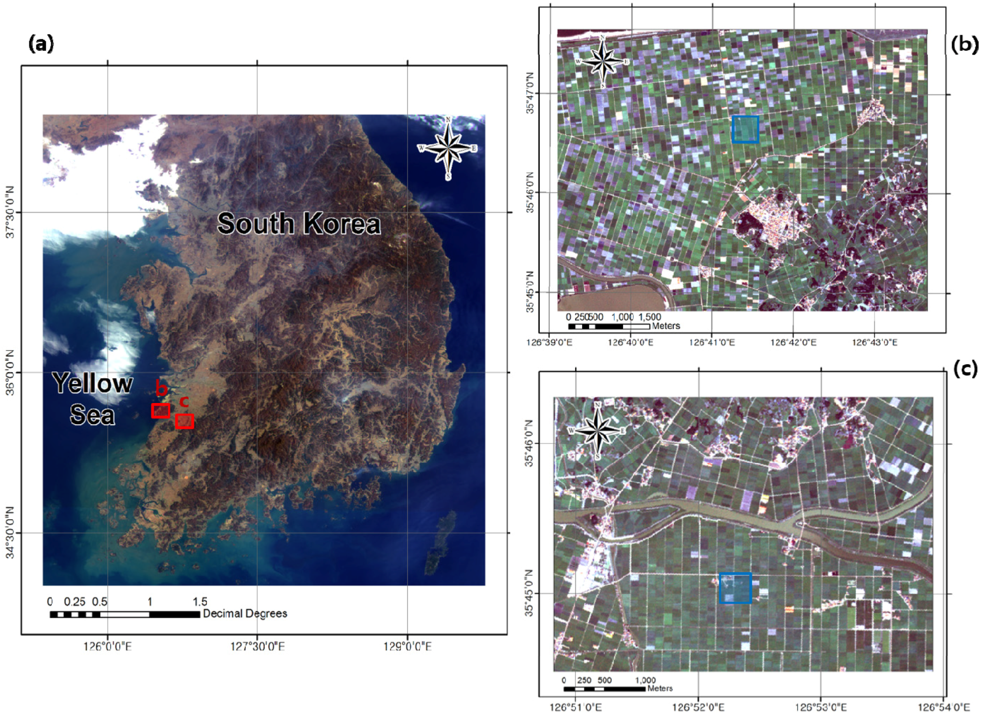
In this study, two paddy rice areas were selected; one was located in Kyehwa and corresponds to a GOCI pixel with coordinates of 35°46′37N and 126°41′03E (Figure 1b). The other was in Kimjae and corresponds to a GOCI pixel with coordinates of 35°44′59N and 126°52′15E (Figure 1c). These paddy areas were included in the monitoring site for the rice yield estimation by the Korea Agricultural Research & Extension Services. The study site at Kimjae represents the double cropping of barley and early maturing rice cultivars, and the site in Kyehwa represents the most popular paddy rice agriculture with an intermediate-late-maturing rice cultivar. The early maturing rice cultivars are generally transplanted a little later than intermediate-late-maturing species, around the middle of June, and harvested at the end of September or the beginning of October. The intermediate-late rice cultivars are transplanted from the end of May until the beginning of June and harvested around the middle of October. As these study sites are relatively homogeneous, despite the small paddy units, the temporal dynamics of different crops should be recognizable in the daily satellite image data analysis.

Figure 1. Study area. (a) Red Green Blue (RGB) color composite image from the Geostationary Ocean Color Imager (GOCI) acquired on 1 April 2011. The red rectangles, (b) and (c), in (a) are shown in (b), and (c), respectively, giving detailed views using high-resolution RapidEye multispectral data obtained on 5 August 2011 (b), and 11 October 2011 (c). The blue rectangles in (b), and (c) are geometrically matched with corresponding satellite observation pixels.

Figure 1. Study area. (a) Red Green Blue (RGB) color composite image from the Geostationary Ocean Color Imager (GOCI) acquired on 1 April 2011. The red rectangles, (b) and (c), in (a) are shown in (b), and (c), respectively, giving detailed views using high-resolution RapidEye multispectral data obtained on 5 August 2011 (b), and 11 October 2011 (c). The blue rectangles in (b), and (c) are geometrically matched with corresponding satellite observation pixels.

2.2. Satellite Data Used in the Present Study

We compared two sets of optical earth observation satellite data with the same spatial resolution of 500 m; one was from a geostationary (GOCI) and the other from a sun-synchronous satellite (MODIS). GOCI is limited to a 2500 × 2500 km² field of view (FOV) centered with respect to the Korean Peninsula and its eight multispectral bands cover visible and near-infrared (NIR) spectral wavelengths (Table 1). In addition, its geometric accuracy is better than 0.4 pixels. The GOCI viewing zenith angle (VZA) ranges from 32.38° to 63.74°. The GOCI VZA for the study areas was 48.47 (Figure 1b) and 48.46 (Figure 1c). We used the fifth and eighth GOCI bands for calculating the normalized difference vegetation index (NDVI). For comparison, MODIS NDVI products were applied as a reference. This study analyzed the data for the years 2011 to 2014.

Table 1. Detailed characteristics of the GOCI and MODIS sensors used for estimating land-surface products.

Satellite Sensor	Orbit Type	Altitude	Wavelength	Spatial Resolution
GOCI	Geo-synchronous	≈36,000 km	B1: 402–422 nm	Approximately 500 m over South Korea area (≈390 m at nadir)
			B2: 433–453 nm
			B3: 480–500 nm
			B4: 545–565 nm
			B5: 650–670 nm
			B6: 675–685 nm
			B7: 735–755 nm
			B8: 845–885 nm
MODIS	Sun-synchronous	≈705 km	B1: 620–670 nm	500 m at nadir
			B2: 841–876 nm
			B3: 459–479 nm
			B4: 545–565 nm
			B5: 1230–1250 nm
			B6: 1628–1652 nm
			B7: 2105–2155 nm

Table 1. Detailed characteristics of the GOCI and MODIS sensors used for estimating land-surface products.

Satellite Sensor	Orbit Type	Altitude	Wavelength	Spatial Resolution
GOCI	Geo-synchronous	≈36,000 km	B1: 402–422 nm	Approximately 500 m over South Korea area (≈390 m at nadir)
			B2: 433–453 nm
			B3: 480–500 nm
			B4: 545–565 nm
			B5: 650–670 nm
			B6: 675–685 nm
			B7: 735–755 nm
			B8: 845–885 nm
MODIS	Sun-synchronous	≈705 km	B1: 620–670 nm	500 m at nadir
			B2: 841–876 nm
			B3: 459–479 nm
			B4: 545–565 nm
			B5: 1230–1250 nm
			B6: 1628–1652 nm
			B7: 2105–2155 nm

Figure 2 shows the spectral response functions of MODIS (in blue) from MODIS Characterization Support Team and GOCI (in red) from Korea Institute of Ocean Science & Technology (KIOST); the straight and dashed lines in the two colors shown correspond to red and NIR wavelengths, respectively. The spectral response functions (SRFs) shown in Figure 2 for the red and NIR frequencies were slightly different because GOCI was designed to observe ocean products such as chlorophyll. The GOCI visible red band SRF is narrower than that for MODIS because its original band purpose was as a baseline for fluorescence, chlorophyll, and suspended sediment. In this study, interpreting the effect of different SRFs was beyond the scope of our research, requiring sensor calibration with atmospheric constituents and ground spectral information for an accurate reading of the spectral vegetation index from different sensors. We assumed the MODIS spectral bands as a reference and compared them with GOCI land products to determine the feasibility of GOCI land application.

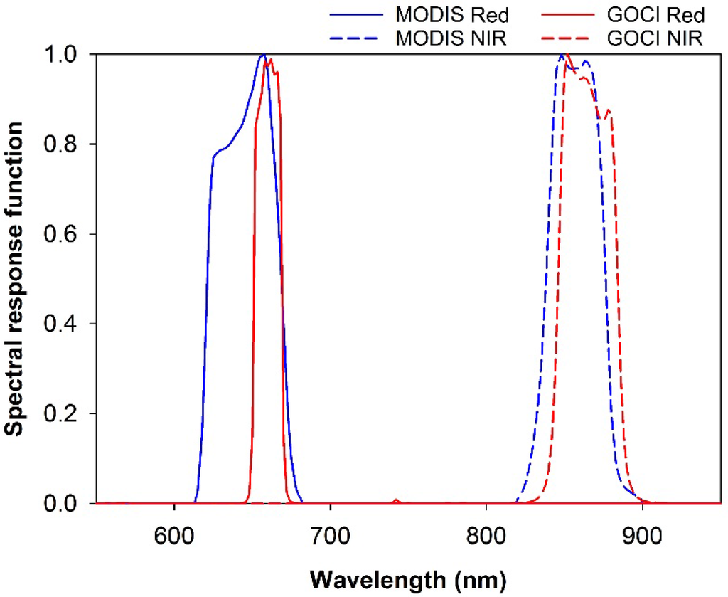
Figure 2. Spectral response function (SRF) of Moderate resolution Imaging Spectroradiometer (MODIS) (in blue) and GOCI (in red). The straight and dashed lines correspond to visible and near-infrared wavelengths, respectively.

Figure 2. Spectral response function (SRF) of Moderate resolution Imaging Spectroradiometer (MODIS) (in blue) and GOCI (in red). The straight and dashed lines correspond to visible and near-infrared wavelengths, respectively.

2.3. Ground Measurements Using a Multispectral Radiometer

In this study, ground measurements were performed using the multispectral radiometer (MSR) to evaluate satellite-based vegetation profiles for comparative analysis. The CROPSCAN MSR16 used in this study was equipped with 16 spectral sensor bands in the 450–1750 nm region. When measuring ground spectral information on rice paddy with CROPSCAN, we observed three different points within selected blue rectangle areas in Figure 1b and 1c, and then averaged the tree points of spectral measurements to reflect spatial representation of chosen rice paddy. The blue rectangles (500 × 500 m) in Figure 1b,c are geometrically matched with corresponding satellite observation pixels for comparison. Field measurements were carried out from June to October 2014. To obtain the crop development characteristics of the paddy rice, measurements were made on eight dates based on the cultivation schedule, including transplantation and harvest. Table 2 lists paddy rice development during the growing season over Kyehwa (Figure 1b) and Kimjae (Figure 1c).

Table 2. Time-series photographs of paddy rice in the Kyehwa and Kimjae areas.

Date	Kyehwa	Kimjae	Status
06/13			After transplantation
06/26			Growing season
07/15			Growing season
07/22			Growing season
08/11			Earing season
08/26			Earing season
09/15			Heading stage
10/03			Harvest

Table 2. Time-series photographs of paddy rice in the Kyehwa and Kimjae areas.

Date	Kyehwa	Kimjae	Status
06/13		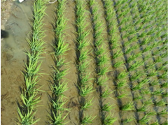	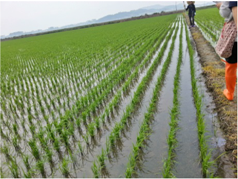After transplantation
06/26		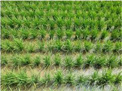	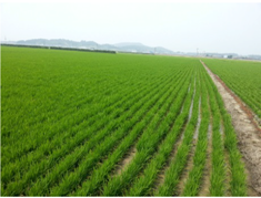Growing season
07/15		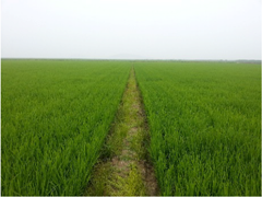	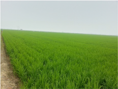Growing season
07/22		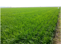	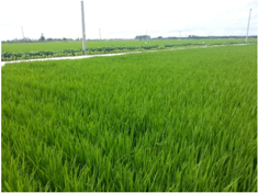Growing season
08/11		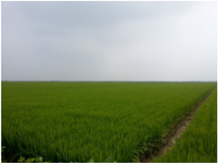	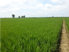Earing season
08/26		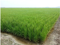	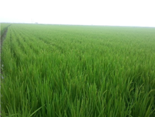Earing season
09/15		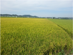	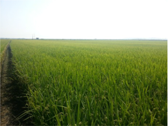Heading stage
10/03		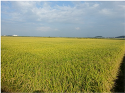	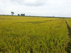Harvest

2.4. Satellite Data Pre-Processing

For the GOCI satellite image, further pre-processing, including conversion of digital numbers (DN) to radiance, cloud masking, and atmospheric correction, was performed to calculate surface reflectance. To undertake cloud masking, a threshold method was adopted [25]. The look-up table (LUT) from the Second Simulation of a Satellite Signal in the Solar Spectral (6S) atmospheric correction model was used for calculating the GOCI surface reflectance [26,27,28]. The 6S radiative transfer model is advantageous for atmospheric correction because it is flexible in applying particular regional characteristics (e.g., topography, land type, or atmospheric condition) and sensor properties (e.g., band width or spectral response function of each band) [29]. The LUT is preliminarily constructed to invert 6S radiative transfer model for calculating the surface reflectance. When simulating 6S modeling for GOCI, atmospheric products such as aerosol optical thickness, aerosol type, ozone, and water vapor were acquired from MODIS atmospheric products (MOD04, MOD05, and MOD07) from NASA’s Earth Observing System Data an Information System (EOSDIS). When using MODIS atmospheric products, which did not fully cover the GOCI observation times, we assumed that the daily variation in the atmospheric constituents from the MODIS atmospheric products was low. When comparing ground station particulate matter (PM_2.5), we found that the overall root mean square error (RMSE) of the aerosol optical depth (AOD) was 0.123 [30]; it follows that the expected error in the surface reflectance using the MODIS daily AOD will be less than 3% in the 6S radiative transfer model. When MODIS products were unavailable (mainly due to cloud contamination), we substituted the aerosol optical thickness based on COMS MI [31] for the MODIS aerosol optical thickness. In this study, for the MODIS satellite image, the MODIS atmospheric corrected reflectance (MOD09GA, MYD09GA, collection 5) from NASA’s EOSDIS was used to estimate the normalized NDVI products. For geometric matching, we applied the nearest-neighbor method to the GOCI and MODIS data by resampling different projected images. Since reflectance measurements from satellite data are affected by the surface anisotropy, the semi-empirical bidirectional reflectance distribution function (BRDF) model was applied to normalize surface reflectance from GOCI and MODIS images.

2.5. BRDF Modeling and Calculation of Vegetation Index

We applied the BRDF model based on Ross-thick/Li-sparse reciprocal (RTLSR) kernels to estimate the normalized reflectance [32,33,34] and correct surface anisotropy effects. Surface reflectance data from GOCI and MODIS were used in the BRDF model to calculate the GOCI and MODIS BRDF-adjusted reflectance, respectively [35,36,37]. The BRDF model kernel coefficients were estimated independently for each gridded pixel location using available cloud-cleared observations for a 16-day composite period to estimate daily rolling products [34,35]. In other words, the cloud-free surface reflectance during the 16-day composite period was assembled to simulate the BRDF model, and then the estimated kernel coefficients were utilized to retrieve the angle-adjusted reflectance. In this study, BRDF-adjusted reflectances from GOCI and MODIS were estimated using a daily rolling strategy over a 16-day composite period to interpret more subtle characteristics of the phenology [36,38]. The BAR products, which were less sensitive to variations in the sun and viewing geometry, were used to estimate daily NDVI products using the following equation:

$$NDV{I}_{BAR}=\frac{NI{R}_{BAR}-re{d}_{BAR}}{NI{R}_{BAR}+re{d}_{BAR}}$$

(1)

where NDVI_BAR is the vegetation index based on BRDF-adjusted surface reflectance, and NIR_BAR and red_BAR represent the BRDF-corrected surface NIR and red bands, respectively.

Lastly, the 10-day NDVI maximum value composite (MVC) is also estimated for comparing the GOCI BAR NDVIs with the GOCI 10-day MVC NDVI. The 10-day NDVI MVC method has been recommended in many cases to minimize the effect of cloud contamination on optical sensors [39] because the highest NDVI value during the 10-day period is retained under the assumption that it represents the NDVI value least affected by the presence of clouds, smoke, haze, snow, and ice during the composite period.

3. Results and Discussion

3.1. Spectral Analysis of Crop Temporal Dynamics

The temporal changes in BAR NDVIs in the four-year GOCI data were compared with those in the corresponding MODIS NBAR NDVIs data for two rice paddies, shown in Figure 1b,c. As Figure 3 shows, the annual NDVI changes correspond well with the crop development of the intermediate-late-maturing rice paddy (Figure 3a), and early maturing rice paddy (Figure 3b).

For the intermediate-late-maturing rice paddy in Figure 3a, compared with the NBAR NDVIs derived from MODIS (solid circles), the GOCI BAR NDVI (open circles) better reflects the annual tendency with less scattering from general crop seasonal dynamics. The advantages of the GOCI are particularly during the summer from June to August, when the weather conditions are very changeable, and rain can persist for long periods. Whereas MODIS resulted in intermittent NDVI values during the long rainy periods (light gray areas in Figure 3) usually between middle June and early August, GOCI provided increasing NDVI values, which appear reasonable for the growing season of paddy rice. In addition, as shown in Figure 3a, the single crop development patterns from the GOCI BAR NDVIs and MODIS NBAR NDVI were similar, but exhibited more discontinuous crop signal transitions of MODIS during the summer from June to August. For the early maturing rice paddy, double cropping spectral patterns were detected (see Figure 3b) for both GOCI (open circles) and MODIS (solid circles). Whereas the GOCI- and MODIS-based vegetation index profiles show similar patterns under benign weather conditions with a high number of angular samples, there is a clear difference between the GOCI- and MODIS-based spectral dynamic patterns during the rainy summer and snowy winter season.

Figure 3. Year-to-year variation in crop seasonal dynamics using GOCI- and MODIS-based vegetation indices. The open and solid circles show the GOCI BAR NDVI and MODIS NBAR NDVI, respectively. The gray and black histograms show the number of GOCI and MODIS angular samples, respectively. (a) Intermediate-late-maturing rice paddy, and (b) Early maturing rice paddy. The four light gray areas from middle June to middle August are rainy summer seasons in South Korea.

Figure 3. Year-to-year variation in crop seasonal dynamics using GOCI- and MODIS-based vegetation indices. The open and solid circles show the GOCI BAR NDVI and MODIS NBAR NDVI, respectively. The gray and black histograms show the number of GOCI and MODIS angular samples, respectively. (a) Intermediate-late-maturing rice paddy, and (b) Early maturing rice paddy. The four light gray areas from middle June to middle August are rainy summer seasons in South Korea.

The quality of BRDF modeling for normalized reflectance is dependent on acquiring at least seven cloud-free observations of each gridded pixel during the 16-day composite period [36]. In Figure 3, the number of cloud-free observations for BRDF modeling is depicted in histograms (gray shows GOCI acquisition and black is MODIS) to ensure the full inversion BRDF parameters required for obtaining reliable surface estimations. If only one to six clear observations are available during the 16-day composite period, then angular sampling numbers of fewer than six were replaced with zero to clearly identify whether full inversion BRDF modeling was applicable. The results from the two study areas show that MODIS (black histogram) did not perform the full inversion with Equation (1) during the rainy season because MODIS from Terra and Aqua can only make two observations over a pixel location. In contrast, GOCI displays exhibited increasing NDVI values during the cloudy summer periods, which appear to be reasonable for the growing seasons (from July to August) of crop areas. As GOCI offers eight multispectral images every day during the daytime (from 9 a.m. to 4 p.m.), the intuitive multi-temporal NDVI can be estimated from sufficient cloud-free observations despite the rainy season.

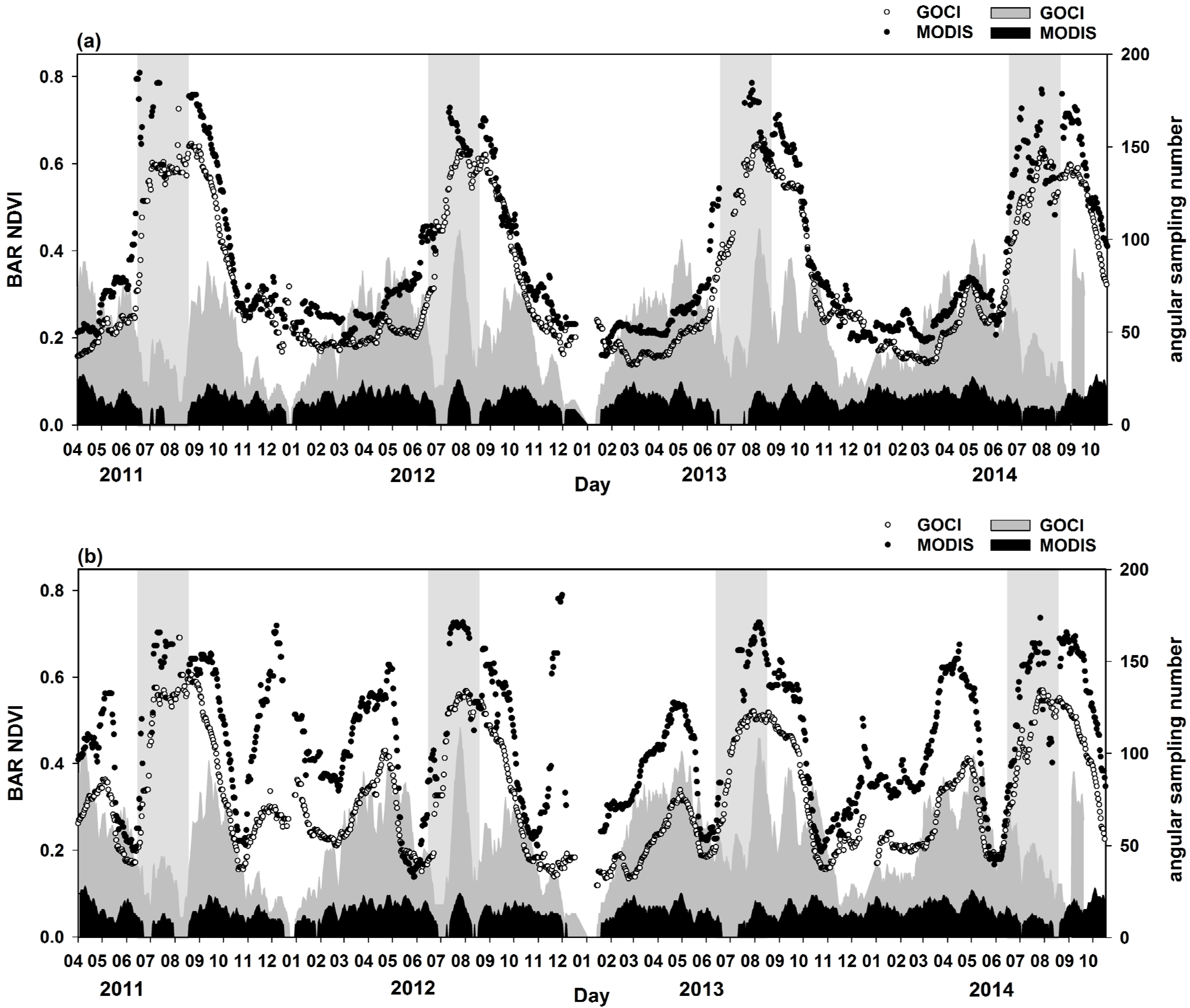
Given the steady margins of the absolute difference between MODIS NBAR NDVIs and GOCI BAR NDVIs under benign weather condition shown in Figure 3, Figure 4 makes one-to-one comparisons of the NDVI, NIR, and Red bands to identify different characteristics of MODIS and GOCI. For both rice paddy areas, GOCI BAR NDVI gave lower values than MODIS, implying that the different SRF of the red band described in Figure 2 might cause the steady margin difference. In Figure 2, NIR SRF had a similar function, but the red band of GOCI has a narrower SRF than MODIS. Therefore, we think that the BAR red band of GOCI gave higher reflectance resulting in lower NDVI values in Figure 4. We inferred that the higher red band RMSE between GOCI and MODIS would cause the higher NDVI RMSE due to SRF different in Figure 4b.

Figure 4. Scatterplots of the GOCI and MODIS vegetation products. The open circles show the BAR NDVI, and the solid and gray circles show the BAR NIR and BAR Red bands, respectively. (a) Intermediate-late maturing rice paddy, and (b) early intermediate-late maturing rice paddy.

Figure 4. Scatterplots of the GOCI and MODIS vegetation products. The open circles show the BAR NDVI, and the solid and gray circles show the BAR NIR and BAR Red bands, respectively. (a) Intermediate-late maturing rice paddy, and (b) early intermediate-late maturing rice paddy.

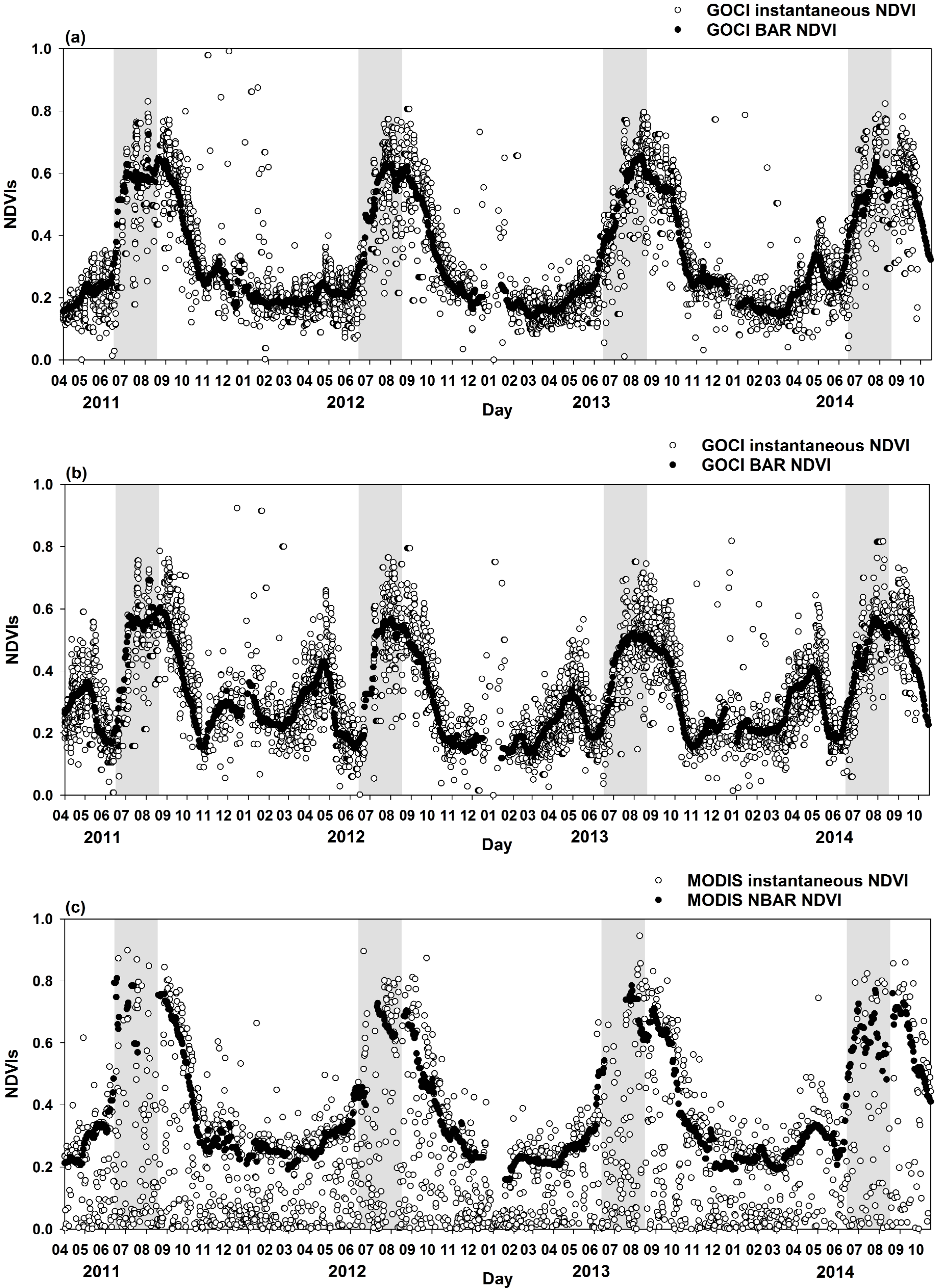
Figure 5 compares two NDVI datasets: one is the instantaneous NDVI measurement from atmospherically corrected reflectance (open circles), and the other is the equivalent processed BAR NDVI (solid circles) for the two crop areas.

For the intermediate-late-maturing rice paddy, the BRDF-adjusted NDVI (solid circles) from GOCI (Figure 5a) and MODIS (Figure 5b) show annual spectral change that corresponds well to the development of vegetation. However, the instantaneous measurements of NDVI from both GOCI and MODIS (open circles) are scattered mostly with the BAR NDVI as the center because of BRDF effects and cloud contamination. For the early maturing rice paddy in Figure 5c,d, similar patterns are shown. In Figure 5, the maximum value of the instantaneous NDVI measurements among the daily values is described alongside the crop dynamics of the study area.

Figure 5. Comparisons of the temporal NDVI variation derived from GOCI and MODIS. The GOCI NDVI profiles for BAR (solid circles) and instantaneous measurement of NDVI (open circles) over (a) intermediate-late maturing paddy rice, and (b) early maturing paddy rice; MODIS NBAR (solid circles) and instantaneous measurement of NDVI (open circles) profiles over (c) intermediate-late-maturing paddy rice, and (d) early maturing paddy rice. The four light gray areas from middle June to middle August are rainy summer seasons in South Korea.

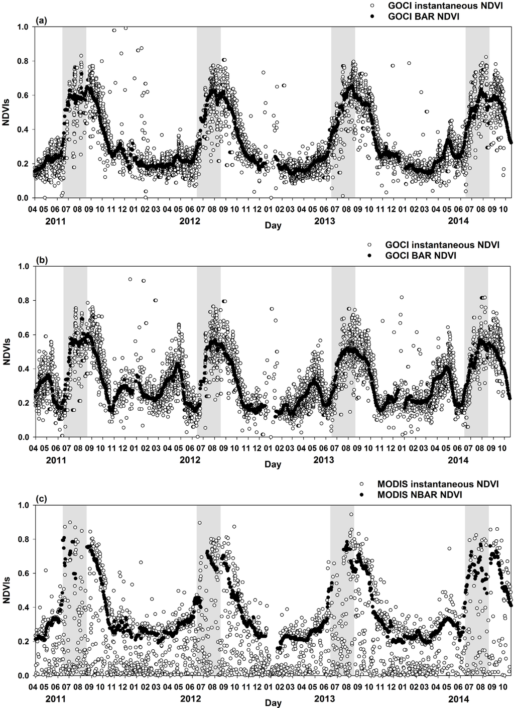
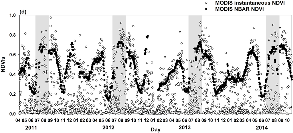
Figure 5. Comparisons of the temporal NDVI variation derived from GOCI and MODIS. The GOCI NDVI profiles for BAR (solid circles) and instantaneous measurement of NDVI (open circles) over (a) intermediate-late maturing paddy rice, and (b) early maturing paddy rice; MODIS NBAR (solid circles) and instantaneous measurement of NDVI (open circles) profiles over (c) intermediate-late-maturing paddy rice, and (d) early maturing paddy rice. The four light gray areas from middle June to middle August are rainy summer seasons in South Korea.

In this study, we also compared the GOCI BAR NDVIs with the GOCI 10-day MVC NDVI based on a daily rolling strategy to determine efficient methods for interpreting intuitive crop dynamics (see Figures 6). The days used to represent these products were the center day of the time window; therefore, matched center data are used for comparison. As shown in Figure 6a, MVC values above 1 were considered outliers, indicating that the MVC method could be used to reveal the limitations associated with minimizing the effect of cloud contamination. However, the crop temporal dynamics of the GOCI 10-day MVC NDVI (open gray circles) did not describe the general phenology pattern, which still remained scattered (Figure 6b). Although scatterplots of the 10-day MVC NDVI displayed better a crop seasonal dynamic pattern compared with the instantaneous measurement NDVI, it was still insufficient with regards to obtaining detailed crop growth and development information, such as the time required for the onset of green-up, the maximum rate of green-up, and time-integrated NDVI as a measure of net primary productivity. For the early maturing rice paddy area, similar characteristics are seen in Figures 6b. Figure 6b shows that the spectral features during the crop-growing season and agricultural off-season are captured in GOCI BAR NDVI, but the crop signal dynamics are not described in the GOCI 10-day MVC NDVI.

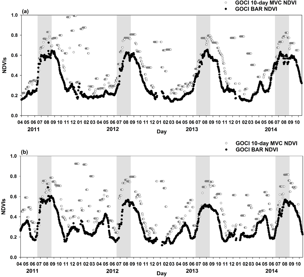
Figure 6. Comparison of the BAR NDVI and 10-day MVC NDVI from GOCI. Temporal variation in BAR NDVI (solid circles) and 10-day MVC NDVI (open gray circles) over intermediate-late-maturing paddy rice (a) and early paddy rice (b). The 4 number of light gray areas from middle June to middle August are rainy summer seasons in South Korea.

Figure 6. Comparison of the BAR NDVI and 10-day MVC NDVI from GOCI. Temporal variation in BAR NDVI (solid circles) and 10-day MVC NDVI (open gray circles) over intermediate-late-maturing paddy rice (a) and early paddy rice (b). The 4 number of light gray areas from middle June to middle August are rainy summer seasons in South Korea.

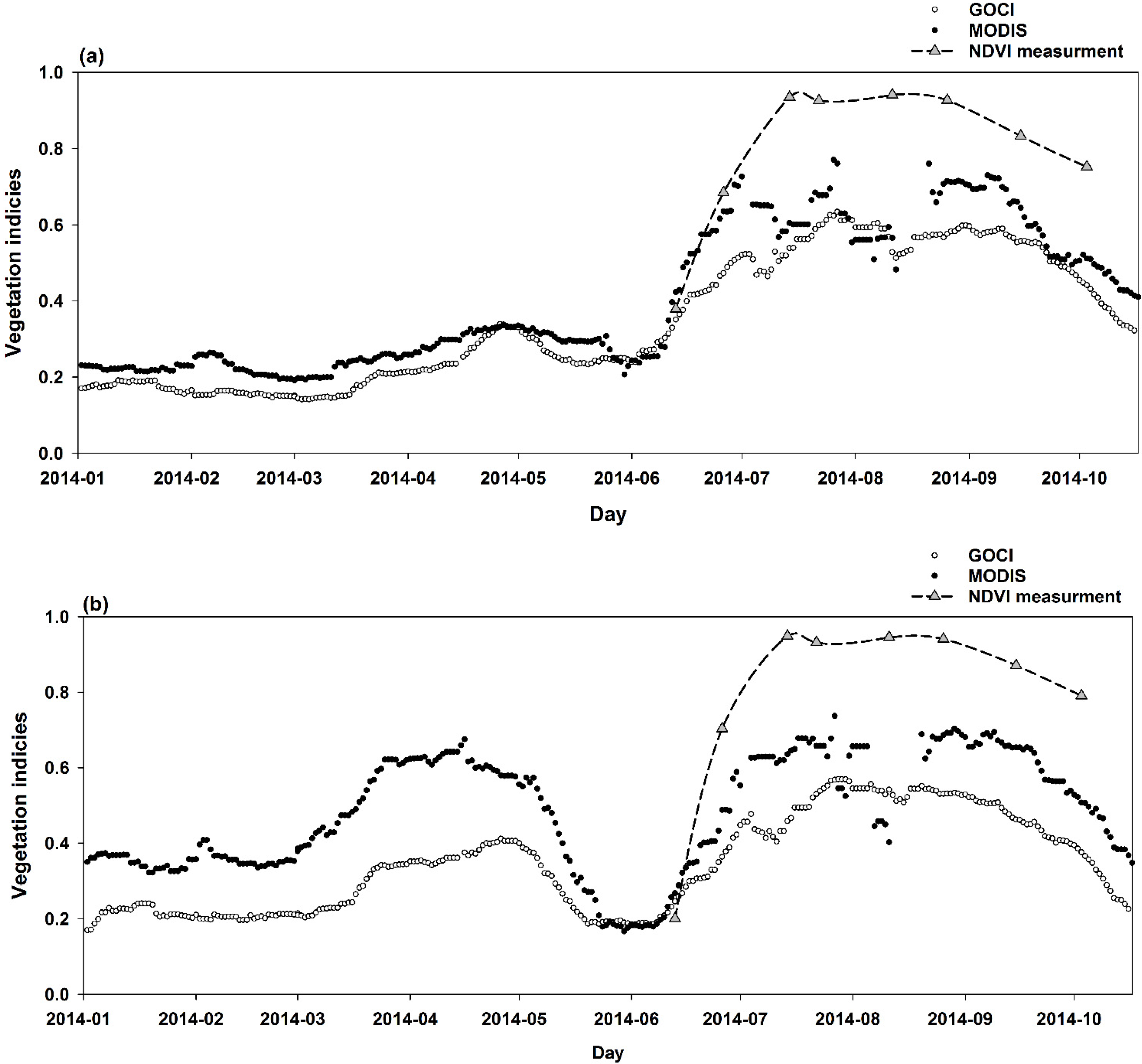
Finally, we compared temporal BRDF-adjusted NDVIs from GOCI and MODIS with field measurement data from CROPSCAN gathered in 2014. Figure 7 shows the comparison of CROPSCAN measured NDVI, interpolated using the cubic spline function (triangle points for measurement and dashed line for interpolated values) and multi-temporal satellite-based NDVIs (open circles for GOCI; solid circles for MODIS) for intermediate-late-maturing rice paddy (Figure 7a) and early-maturing rice paddy (Figure 7b). The field measured NDVIs clearly exhibit higher values than the values based on satellite data values. This may be explained by considering that the CROPSCAN-measured NDVI values represent the coverage of rice planted on a paddy unit whereas the moderate spatial resolution satellite data-based NDVI values include other types of land cover, such as farm roads, vinyl greenhouses, and artificial structures, in its pixel. A comparison without considering the mixed land cover in the MODIS and GOCI data prevents exact validation of the crop temporal dynamics based on the satellite data. However, when interpreted visually, the GOCI BAR NDVI multispectral changes during the growing season appear to better match with the crop development dynamics in the field than the MODIS data. GOCI has similar vegetation trajectory patterns with a constant margin as the CROPSCAN measurement, from date of maximum growth to senescence. However, BRDF adjusted NDVI profiles appeared as shifted to the right side when comparing with the CROPSCAN measurements. It would be caused by the 16-day composite method for simulating BRDF model. BRDF adjusted NDVI might be less sensitive for real time change due to temporal composite than ground measured NDVI representing the immediate reaction of targets.

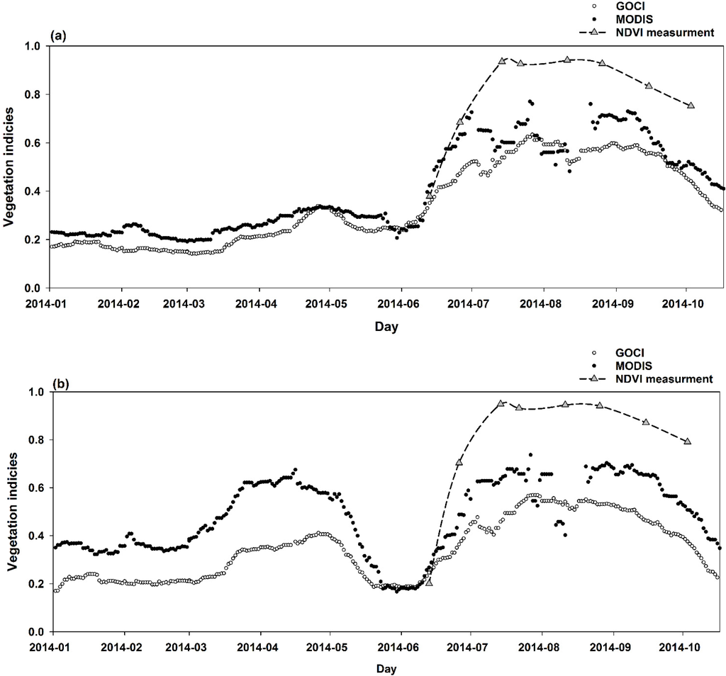
Figure 7. Comparison of temporal BRDF-adjusted NDVI from GOCI (solid circles) and MODIS (open circles) with CROPSCAN measurements (solid triangles) over rice paddy with (a) intermediate-late maturing and (b) early-maturing rice cultivar during 2014. The dashed line over scan measurements is interpolated NDVI using the cubic spline function.

Figure 7. Comparison of temporal BRDF-adjusted NDVI from GOCI (solid circles) and MODIS (open circles) with CROPSCAN measurements (solid triangles) over rice paddy with (a) intermediate-late maturing and (b) early-maturing rice cultivar during 2014. The dashed line over scan measurements is interpolated NDVI using the cubic spline function.

3.2. Discussion

Our four-year GOCI BAR NDVI analysis showed the significant benefit of high temporal resolution for monitoring crop development. However, there were a number of limitations to this work. First, the wavelengths of the red and NIR bands in GOCI and MODIS used for NDVI calculation differed slightly. In principle, for interpreting the different SRFs effects, inter-calibration needs to be performed using stable, homogenous, and less anisotropic natural targets [40]. However, the previous studies revealed the difficulty to compare biophysical products even if derived from the same sensor [41]. So, we performed the one-to-one comparison of the Red, NIR, and NDVI products in order to complement the SRFs difference between GOCI and MODIS and found that the different SRF of the red band might cause the steady margin difference. The interesting fact in the one-to-one comparison was that the BRDF adjusted reflectance showed mostly the less relations, while the NDVIs were well correlated.

Second, there were only two sample sites, and each sample site corresponded to one satellite image pixel. As the main purpose of our study is rapidly to test the benefits of GOCI data with a very high temporal resolution for extracting reliable crop temporal dynamics, we focused on selecting representative study sites instead of quantitative number of study sites. We very carefully chose those two rice paddy sample sites, which are homogeneous despite of small paddy units and covered by the monitoring site for the rice yield estimation by Korea Agricultural Research & Extension Services.

Third, for the comparison of the NDVI calculated using moderate-resolution satellite data with the field measurements, it is necessary to consider the mixed-pixel problem. Because the paddy units in South Korea are relatively very small, it is very difficult to observe a non-mixed spectral value for rice paddies on the moderate spatial resolution GOCI data. The challenges of insufficient spatial resolution were also mentioned in many other studies [42].

4. Conclusion

We investigated the applicability of high-temporal-resolution GOCI satellite data for monitoring crop development. We found that the high temporal resolution of GOCI is advantageous for simulating full inversion BRDF modeling and detecting crop temporal dynamics, which is useful in crop phenology analysis, particularly during the rainy season. In general, GOCI and MODIS displayed similar temporal variation in NDVI under benign weather conditions, because they can secure enough cloud-free observations for full inversion BRDF modeling. During the monsoon season, however, with its long periods of rain and many cloudy days, GOCI was found to be more useful for extracting cloudless or less cloudy areas by arraying its eight images to calculate representative daily data. We also found that the GOCI BAR NDVI was more useful for crop signal monitoring than the widely used MVC NDVI. Lastly, we compared the multi-year NDVI profiles derived from GOCI and MODIS data with field measurements and visually verified the similar crop development patterns between satellite data and field measurement, despite of their different index magnitude.

So, we could conclude that GOCI’s very high-temporal-resolution originally desired for ocean color monitoring is also very applicable for terrestrial monitoring. For the GOCI BAR NDVI, it would be useful to calculate the crop temporal dynamics in greater detail, including the time required for the onset of green-up, maximum rate of green-up, and time-integrated NDVI as a measure of net primary productivity.

We expect that stable vegetation profiles derived from high-temporal-resolution GOCI data will be useful for analyzing crop phenology, as well as phonological parameters reflecting the exact field conditions, which will be the subject of future study. To ensure the GOCI application for land areas, the future study will (1) expand the spatial coverage at a regional or continental scale to show the spatial representativeness, (2) verify the spectral values derived from GOCI and MODIS with ground based spectral measurements to model the real crop development, and lastly (3) simulate the rice yield using GOCI BAR NDVIs and verify its applicability.

References

- Reed, B.; Brown, J.F.; Vanderzee, D.; Loveland, T.R.; Merchant, J.W.; Ohlen, D.O. Measuring phenological variability from satellite imagery. J. Veg. Sci. 1994, 5, 703–714. [Google Scholar]
- Schwartz, M.D.; Ahas, R.; Aasa, A. Onset of spring starting earlier across the Northern hemisphere. Int. J. Climatol. 2006, 22, 343–351. [Google Scholar] [CrossRef]
- Cleland, E.E.; Chuine, I.; Menzel, A.; Nooney, H.A.; Schwartz, M.D. Shifting plant phenology in response to global change. Trends Ecol. Evol. 2007, 22, 357–365. [Google Scholar] [CrossRef] [PubMed]
- Shuai, Y.; Schaaf, C.B.; Zhang, X.; Strahler, A.; Roy, D.; Morisette, J.; Wang, Z.; Nightingale, J.; Nickeson, J.; Richardson, A.D.; et al. Daily MODIS 500 m reflectance anisotropy direct broadcast (DB) products for monitoring vegetation phenology dynamics. Int. J. Remote Sens. 2013, 34, 5997–6016. [Google Scholar] [CrossRef]
- John, F.H.; Robert, W.J.; Bethany, A.B.; John, F.M. Extracting phenological signals from multiyear AVHRR NDVI time series: Framework for applying high-order annual splines with roughness damping. IEEE Trans. Geosci. Remote Sens. 2007, 45, 3264–3276. [Google Scholar]
- Ganguly, S.; Friedl, M.; Tan, B.; Zhang, X.; Verma, M. Land surface phenology from MODIS: characterization of the Collection 5 global land cover dynamics product. Remote Sens. Environ. 2010, 114, 1805–1816. [Google Scholar] [CrossRef]
- Jin, J.; Jiang, H.; Zhang, X.; Wang, Y. Characterizing spatial-temporal variations in Vegetation phenology over the North-South transect of Northeast Asia based upon the MERIS terrestrial chlorophyll index. Terr. Atmos. Ocean. Sci. 2012, 23, 413–424. [Google Scholar] [CrossRef]
- Vintrou, E.; Bégué, A.; Baron, C.; Saad, A.; Seen, D.L.; Traoré, S.B. A comparative study on satellite- and model-based crop phenology in West Africa. Remote Sens. 2014, 6, 1367–1389. [Google Scholar] [CrossRef]
- Delbart, N.; Toan, T.L.; Kergoat, L.; Fedotova, V. Remote sensing of spring phenology in boreal regions: A free of snow-effect method using NOAA-AVHRR and SPOT-VGT data (1982–2004). Remote Sens. Environ. 2006, 101, 52–62. [Google Scholar] [CrossRef]
- Atzberger, C.; Eilers, P.H.C. A time series for monitoring vegetation activity and phenology at 10-daily time steps covering large parts of South America. Int. J. Digit. Earth 2011, 4, 365–386. [Google Scholar] [CrossRef]
- Boschetti, M.; Nutini, F.; Manforn, G.; Brivio, P.A.; Nelson, A. Comparative analysis of normalized difference spectral indices derived from MODIS for detecting surface water in flooded rice cropping systems. PloS ONE. 2014, 9, 1–21. [Google Scholar] [CrossRef] [PubMed]
- Boschetti, M.; Stroppiana, D.; Brivio, P.A.; Bocchi, S. Multi-year monitoring of rice crop phenology through time series analysis of MODIS images. Int. J. Remote Sens. 2009, 30, 4643–4662. [Google Scholar] [CrossRef]
- Sakamoto, T.; Nguyen, N.V.; Ohno, H.; Ishitsuka, N.; Yokozawa, M. Spatio-temporal distribution of rice phenology and cropping systems in the Mekong Delta with spectral reference to the seasonal water flow of the Mekong and Bassac rivers. Remote Sens. Environ. 2006, 100, 1–16. [Google Scholar] [CrossRef]
- Sari, D.K.; Ismullah, I.H.; Sulasdi, W.N.; Harto, A.B. Detecting rice phenology in paddy fields with complex cropping pattern using time series MODIS data. ITB J. Sci. 2010, 42, 91–106. [Google Scholar] [CrossRef]
- Friedl, M.A.; Mclver, D.K.; Hodges, J.C.F.; Zhang, X.Y.; Muchoney, D.; Strahler, A.H.; Woodcock, C.E.; Gopal, S.; Schneider, A.; Cooper, A.; et al. Global land cover mapping from MODIS: Algorithms and early results. Remote Sens. Environ. 2002, 83, 287–302. [Google Scholar] [CrossRef]
- Rembold, F.; Atzberger, C.; Savin, I.; Rojas, O. Using low resolution satellite imagery for yield prediction and yield anomaly detection. Remote Sens. 2013, 5, 5572–5573. [Google Scholar] [CrossRef]
- Viovy, N.; Arino, O.; Belward, A.S. The best index slope extraction (BISE): A method for reducing noise in NDVI time-series. Int. J. Remote Sen. 1992, 13, 1585–1590. [Google Scholar] [CrossRef]
- Roerink, G.J.; Menenti, M.; Verhoef, W. Reconstructing cloud free NDVI composites using Fourier analysis of time series. Int. J. Remote Sen. 2000, 21, 1911–1917. [Google Scholar] [CrossRef]
- Jakubauskas, M.E.; Legates, D.R.; Kastens, J.H. Harmonic analysis of time-series AVHRR NDVI data. Photogramm. Eng. Remote Sens. 2001, 67, 461–470. [Google Scholar]
- Jonsson, P.; Eklundh, L. Seasonality extraction by function fitting to time-series of satellite sensor data. IEEE Trans. Geosci. Remote Sens. 2002, 40, 1824–1832. [Google Scholar] [CrossRef]
- Beck, P.S.A.; Atzberger, C.; Høgda, K.A.; Johansen, B.; Skidmore, A.K. Improved monitoring of vegetation dynamics at very high latitudes: A new method using MODIS NDVI. Remote Sens. Environ. 2006, 100, 321–334. [Google Scholar] [CrossRef]
- Chen, J.M.; Deng, F.; Chen, M.Z. Locally adjusted cubic-spline capping for reconstructing seasonal trajectories of a satellite-derived surface parameter. IEEE Trans. Geosci. Remote Sens. 2006, 44, 2230–2238. [Google Scholar] [CrossRef]
- Hird, J.N.; McDermid, G.J. Noise reduction of NDVI time series: An empirical comparison of selected techniques. Remote Sens. Environ. 2009, 113, 248–258. [Google Scholar] [CrossRef]
- Atkinson, P.M.; Jeganathan, C.; Dash, J.; Atzberger, C. Inter-comparison of four models for smoothing satellite sensor time-series data to estimate vegetation phenology. Remote Sens. Environ. 2012, 123, 400–417. [Google Scholar] [CrossRef]
- Saunders, R.W.; Kriebel, K.T. An improved method for detecting clear sky and cloudy radiances from AVHRR data. Int. J. Remote Sens. 1988, 9, 123–150. [Google Scholar] [CrossRef]
- Vermote, E.F.; Tanre, D.; Deuze, J.L.; Herman, M.; Morcette, J.J. Second simulation of the satellite signal in the solar spectrum, 6S: An overview. IEEE Trans. Geosci. Remote Sens. 1997, 35, 675–686. [Google Scholar] [CrossRef]
- Wang, M. An efficient method for multiple radiative transfer computations and the lookup table generation. J. Quant. Spectrosc. Radiat. Transf. 2003, 78, 471–480. [Google Scholar] [CrossRef]
- Lyapustin, A.; Martonchik, J.; Wang, Y.; Laszlo, I.; Korkin, S. Multiangle implementation of atmospheric correction (MAIAC): 1. Radiative transfer basis and look-up tables. J. Geophys. Res. 2011. [Google Scholar] [CrossRef]
- Lee, C.S.; Yeom, J.M.; Lee, H.L.; Kim, J.J.; Han, K.S. Sensitivity analysis of 6S-based look-up table for surface reflectance retrieval. Asia-Pac. J. Atmos. Sci. 2015, 51, 91–101. [Google Scholar] [CrossRef]
- Green, M.; Kondragunta, S.; Xu, P.C.; Xu, C. Comparison of GOES and MODIS aerosol optical depth (AOD) to aerosol robotic network (AERONET) AOD and IMPROVE PM2.5 mass at Bondville, Illinois. J. Air Waste Manage. Assoc. 2009, 59, 1082–1091. [Google Scholar] [CrossRef]
- Kim, Y.J.; Ahn, M.H.; Sohn, B.J.; Lim, H.S. Retrieving aerosol optical depth using visible and mid-IR channels from geostationary satellite MTSAT-1R. Int. J. Remote Sens. 2008, 29, 6181–6192. [Google Scholar] [CrossRef]
- Roujean, J.L.; Leroy, M.; Deschamps, P.Y. A bidirectional reflectance model of the Earth’s surface for the correction of remote sensing data. J. Geophys. Res. 1992, 97, 20455–20468. [Google Scholar] [CrossRef]
- Wanner, W.; Li, X.; Strahler, A.H. On the derivation of kernels for kernel-driven models of bidirectional reflectance. J. Geophys. Res. 1995, 100, 21077–21089. [Google Scholar] [CrossRef]
- Schaaf, C.B.; Gao, F.; Strahler, A.H.; Lucht, W.; Li, X.; Tsang, T.; Strugnell, N.C.; Zhang, X.; Jin, Y.; Muller, J.P.; et al. First operational BRDF, albedo and nadir Reflectance Products from MODIS. Remote Sens. Environ. 2002, 83, 135–148. [Google Scholar] [CrossRef]
- Lucht, W.; Schaaf, C.B.; Strahler, A.H. An Algorithm for the retrieval of albedo from space using semiempirical BRDF Models. IEEE Trans. Geosci. Remote Sens. 2000, 38, 977–998. [Google Scholar] [CrossRef]
- Shuai, Y.; Schaaf, C.B.; Strahler, A.H.; Liu, J.; Jiao, Z. Quality assessment of BRDF/Albedo retrievals in MODIS operational system. Geophys. Res. Lett. 2008, 35, L05407. [Google Scholar] [CrossRef]
- Yeom, J.M.; Kim, H.O. Feasibility of using Geostationary Ocean Color Imager (GOCI) data for land applications after atmospheric correction and bidirectional reflectance distribution function modelling. Int. J. Remote Sens. 2013, 34, 7329–7339. [Google Scholar] [CrossRef]
- Ju, J.; Roy, D.; Shuai, Y.; Schaaf, C.B. Development of an approach for generation of temporally complete daily nadir MODIS reflectance time series. Remote Sens. Environ. 2010, 114, 1–20. [Google Scholar] [CrossRef]
- Holben, B.N. Characteristics of maximum-value composite images from temporal AVHRR data. Int. J. Remote Sens. 1986, 7, 1417–1434. [Google Scholar] [CrossRef]
- Chander, G.; Hewison, T.J.; Fox, N.; Wu, X.; Xiong, X.; Blackwell, W.J. Overview of intercalibration of satellite instruments. IEEE Trans. Geosci. Remote Sens. 2013, 51, 1056–1080. [Google Scholar] [CrossRef]
- Meroni, M.; Atzberger, C.; Vancutsem, C.; Gobron, N.; Baret, F.; Lacaze, R.; Eerens, H.; Leo, O. Evaluation of agreement between space remote sensing SPOT-VEGETATION fAPAR time series. IEEE Trans. Geosci. Remote Sens. 2013, 51, 1951–1932. [Google Scholar] [CrossRef]
- Ozdogan, M. The spatial distribution of crop types from MODIS data: Temporal unmixing using independent component analysis. Remote Sens. Environ. 2010, 114, 1190–1204. [Google Scholar] [CrossRef]
© 2015 by the authors; licensee MDPI, Basel, Switzerland. This article is an open access article distributed under the terms and conditions of the Creative Commons Attribution license (http://creativecommons.org/licenses/by/4.0/).